Hard-Loop Dynamics of Non-Abelian Plasma Instabilities

Abstract

Non-Abelian plasma instabilities may be responsible for the fast apparent quark-gluon thermalization in relativistic heavy-ion collisions if their exponential growth is not hindered by nonlinearities. We study numerically the real-time evolution of instabilities in an anisotropic non-Abelian plasma with an SU(2) gauge group in the hard-loop approximation. We find exponential growth of non-Abelian plasma instabilities both in the linear and in the strongly nonlinear regime, with only a brief phase of subexponential behavior in between.

In this Letter we present first results on the real-time evolution of non-Abelian plasma instabilities due to momentum-space anisotropies in the underlying quark and gluon distribution functions Stan:9397 ; Mrowczynski:2000ed ; RM:2003 ; Romatschke:2003ms ; Arnold:2003rq ; Mrowczynski:2004kv ; Arnold:2004ih in the nonlinear hard-loop approximation. Such anisotropies are generated during the natural expansion of the matter created during a heavy-ion collision and the resulting instabilities may be responsible for the fast apparent thermalization Arnold:2004ti , which seems to be faster than can be accounted for by perturbative scattering processes Baier:2000sb ; Molnar:2001ux ; Heinz:2004pj ; Shuryak:2004kh . This type of plasma instability is the analogue of the electromagnetic Weibel instability which causes soft gauge (magnetic) fields to become nonperturbatively large. Eventually this leads to large-angle scattering of hard particles Weibel:1959 , thereby rapidly accelerating the isotropization and subsequent thermalization of an Abelian plasma with a temperature anisotropy. However, in the non-Abelian case it is conceivable that the intrinsic nonlinearities could cause the instabilities to stop growing before they have large effects on hard particles and therefore reduce their efficacy in isotropizing a non-Abelian plasma.

The regime where the backreaction of collective fields on the hard particles is still weak but where the self-interaction of the former may already be strongly nonlinear is governed by a “hard-loop” effective action which has been derived in Ref. Mrowczynski:2004kv for arbitrary momentum-space anisotropies . We discretize this effective action in a local auxiliary-field formulation, keeping its full dynamical nonlinearity and nonlocality. This is then applied to initial conditions that allow for an effectively 1+1-dimensional lattice simulation, extending a previous numerical study Arnold:2004ih that used a static and linear approximation to the hard-loop effective action.

Discretized Hard-Loop Dynamics.—At weak gauge coupling $g$, there is a separation of scales in hard momenta $|\mathbf{p}|=p^{0}$ of (ultrarelativistic) plasma constituents, and soft momenta $\sim g|\mathbf{p}|$ pertaining to collective dynamics. The effective field theory for the soft modes that is generated by integrating out the hard plasma modes at one-loop order and in the approximation that the amplitudes of the soft gauge fields obey $A_{\mu}\ll|\mathbf{p}|/g$ is that of gauge-covariant collisionless Boltzmann-Vlasov equations HTLreviews . In equilibrium, the corresponding (nonlocal) effective action is the so-called hard-thermal-loop effective action HTLeffact which has a simple generalization to plasmas with anisotropic momentum distributions Mrowczynski:2004kv . Its contribution to the effective field equations of soft modes is an induced current of the form Blaizot:1993be ; Mrowczynski:2000ed

$$j^{\mu}[A]=-g^{2}\int{d^{3}p\over(2\pi)^{3}}{1\over 2|\mathbf{p}|}\,p^{\mu}\,{\partial f(\mathbf{p})\over\partial p^{\beta}}W^{\beta}(x;\mathbf{v}),$$ (1)

where $f$ is a weighted sum of the quark and gluon distribution functions Mrowczynski:2004kv . The quantities $W_{\beta}(x;\mathbf{v})$ satisfy

$$[v\cdot D(A)]W_{\beta}(x;\mathbf{v})=F_{\beta\gamma}(A)v^{\gamma}\,$$ (2)

with $v^{\mu}\equiv p^{\mu}/|\mathbf{p}|=(1,\mathbf{v})$, $D_{\mu}=\partial_{\mu}-ig[A_{\mu},\cdot]$, metric convention $(+---)$, and this has to be solved self-consistently with $D_{\mu}(A)F^{\mu\nu}=j^{\nu}$. At the expense of having introduced a continuous set of auxiliary fields $W_{\beta}(x;\mathbf{v})$ the effective field equations are local, but nonlinear in the case of a non-Abelian gauge theory.

We shall be interested in particular in the case where there is just one direction of momentum-space anisotropy (e.g., the collision axis in heavy-ion experiments), so we assume cylindrical symmetry and parametrize the first derivatives of the hard particle distribution function by

$${\partial f(\mathbf{p})\over\partial p^{\beta}} = {\partial f(|\mathbf{p}|,p^{z})\over\partial|\mathbf{p}|}{p^{b}\delta_{b\beta}\over|\mathbf{p}|}+{\partial f(|\mathbf{p}|,p^{z})\over\partial p^{z}}\delta_{z\beta}$$ (3)

$$\equiv -\tilde{f}_{1}(|\mathbf{p}|,p^{z}){p^{b}\delta_{b\beta}\over|\mathbf{p}|}-\tilde{f}_{2}(|\mathbf{p}|,p^{z})\delta_{z\beta}.$$

Because $p^{\beta}W_{\beta}=0$, we have

$$j^{\mu}(x)={1\over 2}g^{2}\int{d^{3}p\over(2\pi)^{3}}v^{\mu}\,[\tilde{f}_{1}W^{0}(x;v)+\tilde{f}_{2}W^{z}(x;v)].$$ (4)

In the isotropic case one has $\tilde{f}_{2}=0$, and only $W^{0}$ appears, whose equation of motion (2) is driven by (chromo)electric fields; in the anisotropic case, however, $W^{z}$ enters, whose equation of motion involves the $z$ component of the Lorentz force.

The induced current (1) is covariantly conserved as one can verify by partial integration with respect to $p^{\beta}$ Mrowczynski:2004kv , but no partial integration is needed for parity invariant distribution functions $f$. This is only a mild restriction on the choice of $f$’s, but a great advantage for the following discretization. For $f(\mathbf{p})=f(-\mathbf{p})$, the two terms in the current (4) are covariantly conserved individually, because Eq. (2) implies that $D\cdot j\propto\int\!{d^{3}p}\,(\tilde{f}_{1}F^{0\gamma}v_{\gamma}+\tilde{f}_{2}F^{z\gamma}v_{\gamma})$, which vanishes by symmetry.

Our aim will be to study the hard-loop dynamics in lattice discretization where we approximate the continuous set of fields $W_{\beta}(x;\mathbf{v})$ by a finite number of fields. Because Eq. (2) does not mix different $v$’s, a closed set of equations is obtained when the integral in Eq. (4) is discretized with respect to directions $\mathbf{v}$

$$j^{\mu}(x) = g^{2}\int{p^{2}dp\over(2\pi)^{2}}{1\over\mathcal{N}}\sum_{\bf v}v^{\mu}\,[\tilde{f}_{1}W^{0}_{\mathbf{v}}(x)+\tilde{f}_{2}W_{\mathbf{v}}^{z}(x)]$$ (5)

$$\equiv{1\over\mathcal{N}}\sum_{\bf v}v^{\mu}[a_{\mathbf{v}}W^{0}_{\mathbf{v}}(x)+b_{\mathbf{v}}W^{z}_{\mathbf{v}}(x)],$$

where the $\mathcal{N}$ unit vectors $\mathbf{v}$ define a partition of the unit sphere in patches of equal area, and where $a_{\mathbf{v}}$, $b_{\mathbf{v}}$ are then fixed coefficients for a given distribution function $f$. Covariant conservation of $j$ is ensured by symmetric choices of the set of $\mathbf{v}$’s which satisfy $\sum_{\mathbf{v}}a_{\mathbf{v}}\mathbf{v}=0$, $\sum_{\mathbf{v}}b_{\mathbf{v}}=0$, and $\sum_{\mathbf{v}}b_{\mathbf{v}}\mathbf{v}_{\perp}=0$, with $\mathbf{v}_{\perp}=\mathbf{v}-v^{z}\mathbf{e}_{z}$.

Given such a discretization, which is a discretization of the phase space of the hard particles with respect to the directions of their momenta, only $\mathcal{N}$ auxiliary fields $\mathcal{W}_{\mathbf{v}}=a_{\mathbf{v}}W^{0}_{\mathbf{v}}+b_{\mathbf{v}}W^{z}_{\mathbf{v}}$ participate in the dynamical evolution. The full hard-loop dynamics is then approximated by the following set of matrix-valued equations,

$$[v\cdot D(A)]\mathcal{W}_{\mathbf{v}}=(a_{\mathbf{v}}F^{0\mu}+b_{\mathbf{v}}F^{z\mu})v_{\mu}$$ (6)

$$D_{\mu}(A)F^{\mu\nu}=j^{\nu}={1\over\mathcal{N}}\sum\limits_{\mathbf{v}}v^{\nu}\mathcal{W}_{\mathbf{v}},$$ (7)

which can be systematically improved by increasing $\mathcal{N}$.

A different possibility for discretizing hard-loop dynamics that has been employed previously in isotropic plasmas would be a decomposition of the auxiliary fields $W^{\mu}(x;v)$ into spherical harmonics Bodeker:1999gx ; Rajantie:1999mp . Our proposal is slightly simpler, but also more flexible in that it allows one to e.g. improve approximations in highly anisotropic cases with cylindrical symmetry by selectively increasing the resolution in $z$ direction more than in $\varphi$ direction.

The dynamical system described by Eqs. (6) and (7) has constant total energy of the form

$$\mathcal{E}=\int d^{3}x\,{\rm tr}\,(\mathbf{E}^{2}+\mathbf{B}^{2})|_{t}+\int_{t_{0}}^{t}\!dt^{\prime}\int d^{3}x\,2\,{\rm tr}\,\mathbf{j}_{t^{\prime}}\cdot\mathbf{E}_{t^{\prime}}.$$ (8)

The part containing the induced current involves

$$\,{\rm tr}\,\mathbf{j}\cdot\mathbf{E} = {g^{2}\over 4}\partial_{\mu}\int{d^{3}p\over(2\pi)^{3}}\tilde{f}_{1}v^{\mu}W_{0}^{2}$$ (9)

$$+{g^{2}\over 2}\int{d^{3}p\over(2\pi)^{3}}\tilde{f}_{2}W^{z}(v\cdot D)W_{0},$$

which shows that in the isotropic case ($\tilde{f}_{2}=0$) there is a local, positive definite energy contribution from the plasma Blaizot:1994am . However, in the general anisotropic case, positivity is lost, corresponding to the possibility of plasma instabilities, where energy may be extracted from hard particles and deposited into the soft collective fields without bound as long as the hard-loop approximation $A_{\mu}\ll|\mathbf{p}|/g$ remains valid.

1+1-dimensional lattice simulation.—When only $z$-dependent initial conditions are imposed, the entire dynamics proceeds 1+1-dimensionally and we can take all collective fields as 1+1-dimensional, though the underlying hard degrees of freedom are of course still 3+1 dimensional, with a discrete set of directions $\mathbf{v}$ for their (conserved) momenta. This dimensionally reduced situation already allows us to study the evolution of non-Abelian Weibel instabilities, which in the linear (Abelian) regime are formed by (superpositions of) transverse standing waves with exponentially growing amplitudes.

We have solved the equations (6) and (7) in this dimensionally reduced situation by lattice discretization, closely following Ref. Arnold:2004ih who considered a toy model corresponding to an induced current which is simply

$$j_{\alpha}^{\rm AL}=\mu^{2}A_{\alpha},\quad\alpha=x,y.$$ (10)

As was shown in Ref. Arnold:2004ih , this reproduces the static limit of the anisotropic hard-loop effective action for fields that vary only in the anisotropy direction, but it neglects its general frequency dependence and dynamical nonlinearity. This is now provided through Eqs. (6) and (7).

Like Ref. Arnold:2004ih we work in temporal axial gauge $A^{0}=0$ and take initial conditions corresponding to small random chromoelectric fields $\mathbf{E}=-\partial_{t}\mathbf{A}$ with polarization transverse to the $z$-axis, and all other fields vanishing, which in our case includes the auxiliary fields $\mathcal{W}_{\mathbf{v}}$. This initial condition satisfies the Gauss law constraint, $\mathbf{D}\cdot\mathbf{E}={\mathcal{N}}^{-1}\sum_{\mathbf{v}}\mathcal{W}_{\mathbf{v}},$ whose continued fulfilment is monitored in the simulation, but not enforced. As a further nontrivial check of our numerics, we tracked conservation of the total energy (8).

In order to be able to compare with the analytical results of Ref. Romatschke:2003ms , we consider an anisotropic distribution function $f=N(\xi)f_{iso}(\mathbf{p}^{2}+\xi p_{z}^{2})$. This determines the coefficients in Eq. (5) according to

$$a_{\mathbf{v}}={m^{2}(1+\xi v_{z}^{2})^{-2}},\qquad b_{\mathbf{v}}=\xi v_{z}a_{\mathbf{v}},$$ (11)

where $m^{2}=N(\xi)m_{D}^{2}(0)$ with $m_{D}(0)$ the Debye mass of the isotropic case $\xi=0$, and $N(\xi)$ a normalization factor which equals $N(\xi)=\sqrt{1+\xi}$ if one requires that the number density of hard particles remains the same for different values $\xi$.

For $\xi>0$ transverse modes with wave vector $|\mathbf{k}|<\mu$,

$$\mu^{2}={1\over 4}\left(1+{\xi-1\over\sqrt{\xi}}\arctan{\sqrt{\xi}}\right)m^{2},$$ (12)

are unstable and grow with a $k$-dependent growth rate $\gamma(k)$, shown in Fig. 1 for $\xi=10$, which has a maximum $\gamma_{*}$ at nonvanishing $|\mathbf{k}|=k_{*}$ and a zero at $\mathbf{k}=0$. By contrast, the growth rate implied by the toy model (10) is given by $\gamma=\sqrt{\mu^{2}-\mathbf{k}^{2}}$, whose maximum is at $\mathbf{k}=0$ and equals $\mu$.

Figure 1: The growth rate $\gamma(k)$ of unstable modes for the discretized hard loops with $\mathcal{N}=100$ (dashed line) in comparison with the continuum result (solid line) for $\xi=10$.

In the linearized case one can also determine the dispersion laws analytically in the case of finite $\mathcal{N}$. Fig. 1 compares the growth rates $\gamma(k)$ for full and discretized hard loops with $\mathcal{N}=\mathcal{N}_{z}\times\mathcal{N}_{\varphi}=20\times 5=100$, which shows that the latter give very accurate approximations for $\mathcal{N}\gtrsim 100$. As another example, the asymptotic mass of the stable propagating modes with $|\mathbf{k}|\gg\mu$ is given for full hard loops by $m^{2}_{\infty}={m^{2}/(2\sqrt{\xi})}\arctan{\sqrt{\xi}}$, which for $\xi=10$, $\mathcal{N}=100$ is reproduced with an error of only 0.017%.

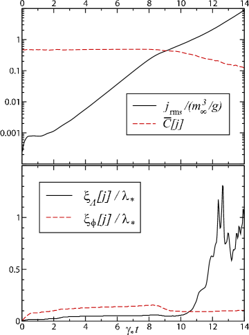
Figure 2: The average current $j_{rms}$ and the average relative size $\bar{C}$ of commutators $[j_{x},j_{y}]$ as a function of time (upper panel); the Abelianization correlation length $\xi_{A}[j]$ and the ordinary correlation length $\xi_{\phi}[j]$, normalized to the scale of maximal growth $\lambda_{*}$ (lower panel).

The results of our lattice simulations of the nonlinear evolution for a gauge group SU(2) are finally shown in Figs. 2 and 3, where we have used the parameters $\xi=10$, $\mathcal{N}_{z}\times\mathcal{N}_{\varphi}=20\times 5$ for discretizing the unit sphere with uniform spacing in $z$ and $\varphi$. The one-dimensional spatial lattice has 10,000 sites, periodic boundary conditions, and lattice spacing corresponding to $am_{\infty}=0.028$ so that the physical size is $L\approx 280\,m_{\infty}^{-1}$. Using a leapfrog algorithm with time steps $\epsilon/a=1/100$, we track the evolution of a single field configuration with random initial seed chromoelectric field of root-mean-square amplitude $0.012\,m_{\infty}^{2}/g$. The Gauss law constraint turns out to remain preserved within machine accuracy; the total energy (8) is conserved within less than 1%, with the percentage level being reached only at the largest times when the energy in the soft fields has grown by more than a factor of $10^{6}$ (full details will be given elsewhere).

The upper panel of Fig. 2 shows the evolution of

$$j_{rms}=\left[\int_{0}^{L}{dz\over L}2\,{\rm tr}\,(\mathbf{j}^{2})\right]^{1/2},$$ (13)

which (after some initial wobble) grows exponentially with a growth rate that is most of the time only slightly below $\gamma_{*}$, except for a transitory reduction at the beginning of the nonlinear regime, when $j_{rms}\sim m_{\infty}^{3}/g$. Also shown is the dimensionless observable $\bar{C}$, defined by

$$\bar{C}=\int_{0}^{L}{dz\over L}{\left\{\,{\rm tr}\,\left((i[j_{x},j_{y}])^{2}\right)\right\}^{1/2}\over\,{\rm tr}\,(j_{x}^{2}+j_{y}^{2})}$$ (14)

and giving a measure of local “non-Abelianness”. In the toy model of Ref. Arnold:2004ih it was found that $\bar{C}$ suddenly begins to decay exponentially when fields get strong, with a decay rate similar to the growth rate of $j_{rms}$. In the hard-loop case, we observe a similar phenomenon, but the decay rate of $\bar{C}$ is much smaller (and also less constant once the decay begins).

Ref. Arnold:2004ih also observed a concurrent global Abelianization, by comparing the correlation among parallel transported spatially separated commutators to the correlation of parallel transported fields. A correlation length $\xi_{A}$ defined through the former was found to rapidly grow to lattice size when $\bar{C}$ begins to decay, whereas no such growth occurred in the general field correlation length $\xi_{\phi}$. In the lower panel of Fig. 2 we show the analogous quantities computed using currents instead of field values [22] and we found that correlated Abelianization takes place over extended domains, which remain bounded, however. In fact, $\xi_{A}$ turns out to be comparable with the scale of maximal growth $\lambda_{*}=2\pi/k_{*}\approx 7m_{\infty}^{-1}$. By contrast, in the model of Ref. Arnold:2004ih $k_{*}$ vanishes, which is presumably responsible for the different global behavior.

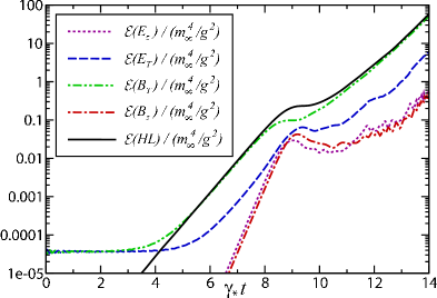
Figure 3: Average energy densities $\mathcal{E}$ in transverse/longitudinal chromomagnetic/electric fields and the total energy density contributed by hard particles, $\mathcal{E}({\rm HL})$.

Fig. 3 shows how the exponentially growing energy transferred from hard to soft scales is distributed among chromomagnetic and chromoelectric collective fields. The dominant contribution is in transverse magnetic fields, and it grows roughly with the maximum rate $\gamma_{*}$ both in the linear as well as in the highly nonlinear regime, with a transitory slowdown in between. Transverse electric fields behave similarly, and are suppressed by a factor of the order of $(\gamma_{*}/k_{*})^{2}$ . The appearance of longitudinal contributions, which are absent in the initial conditions we have chosen, is a purely non-Abelian effect. While completely negligible at first, they have a growth rate which is double the one in the transverse sector, and they begin to catch up with the latter just when local Abelianization sets in. At that stage there appears to be some complicated rearrangement taking place, which delays the exponential evolution by a time $\Delta t\sim\gamma_{*}^{-1}$, but subsequently the growth rate gets restored roughly to its previous value. Eventually there will be a point where the hard-loop approximation breaks down, namely when the energy transferred from hard to soft modes becomes comparable to that initially present in the former.

From the above numerical results on the hard-loop dynamics of non-Abelian plasma instabilities we conclude that the latter do not saturate until they begin to have large effects on hard particle trajectories, even though our simulations indicate complicated dynamics and only limited Abelianization of the unstable modes. Therefore it appears indeed possible that non-Abelian plasma instabilities are responsible for accelerated thermalization in a weakly coupled quark-gluon plasma.

- (1) S. Mrówczyński, Phys. Lett. B 314, 118 (1993); Phys. Rev. C 49, 2191 (1994); Phys. Lett. B 393, 26 (1997).
- (2) S. Mrówczyński and M. H. Thoma, Phys. Rev. D 62 (2000) 036011.
- (3) J. Randrup and S. Mrówczyński, Phys. Rev. C 68, 034909 (2003).
- (4) P. Romatschke and M. Strickland, Phys. Rev. D 68, 036004 (2003); arXiv:hep-ph/0406188.
- (5) P. Arnold, J. Lenaghan and G. D. Moore, JHEP 0308, 002 (2003).
- (6) S. Mrówczyński, A. Rebhan and M. Strickland, Phys. Rev. D 70, 025004 (2004).
- (7) P. Arnold and J. Lenaghan, Phys. Rev. D 70, 114007 (2004).
- (8) P. Arnold, J. Lenaghan, G. D. Moore and L. G. Yaffe, Phys. Rev. Lett. 94, 072302 (2005).
- (9) R. Baier, A. H. Mueller, D. Schiff and D. T. Son, Phys. Lett. B 502, 51 (2001).
- (10) D. Molnar and M. Gyulassy, Nucl. Phys. A 697, 495 (2002) [Erratum-ibid. A 703, 893 (2002)].
- (11) U. W. Heinz, arXiv:nucl-th/0407067.
- (12) E. Shuryak, J. Phys. G 30, S1221 (2004).
- (13) E.S. Weibel, Phys. Rev. Lett. 2, 83 (1959).
- (14) J. P. Blaizot and E. Iancu, Phys. Rept. 359, 355 (2002) and references therein.
- (15) J. C. Taylor and S. M. H. Wong, Nucl. Phys. B 346, 115 (1990); J. Frenkel and J. C. Taylor, Nucl. Phys. B 374, 156 (1992); E. Braaten and R. D. Pisarski, Phys. Rev. D 45, 1827 (1992).
- (16) J. P. Blaizot and E. Iancu, Nucl. Phys. B 417, 608 (1994).
- (17) D. Bödeker, G. D. Moore and K. Rummukainen, Phys. Rev. D 61, 056003 (2000).
- (18) For a more efficient method in the case of Abelian isotropic plasmas see A. Rajantie and M. Hindmarsh, Phys. Rev. D 60, 096001 (1999), who also discussed discretized ’s.
- (19) J. P. Blaizot and E. Iancu, Nucl. Phys. B 421, 565 (1994).