Fittino, a program
for determining MSSM parameters
from collider observables
using an iterative method



P. Bechtle^a,b, K. Desch^a and P. Wienemann<sup>b




a</sup>Institut für Experimentalphysik, Universität Hamburg, Luruper Chaussee 149, D-22761 Hamburg, Germany
^bDeutsches Elektronen-Synchrotron DESY, Notkestr. 85, D-22607 Hamburg, Germany

Provided that Supersymmetry (SUSY) is realized, the Large Hadron Collider (LHC) and the future International Linear Collider (ILC) may provide a wealth of precise data from SUSY processes. An important task will be to extract the Lagrangian parameters. On this basis the goal is to uncover the underlying symmetry breaking mechanism from the measured observables. In order to determine the SUSY parameters, the program Fittino has been developed. It uses an iterative fitting technique and a Simulated Annealing algorithm to determine the SUSY parameters directly from the observables without any a priori knowledge of the parameters, using all available loop-corrections to masses and couplings. Simulated Annealing is implemented as a stable and efficient method for finding the optimal parameter values. The theoretical predictions can be provided from any program with SUSY Les Houches Accord interface. As fit result, a set of parameters including the full error matrix and two-dimensional uncertainty contours are obtained. Pull distributions can automatically be created and allow an independent cross-check of the fit results and possible systematic shifts in the parameter determination. A determination of the importance of the individual observables for the measurement of each parameter can be performed after the fit. A flexible user interface is implemented, allowing a wide range of different types of observables and a wide range of parameters to be used.

1 Introduction

Fittino [1] is a program implemented in $\mathrm{C}\!\!+\!\!+$, which extracts the parameters of the SUSY Lagrangian from (simulated) measurements at future colliders such as the LHC and the ILC in a global fit. It has been created in the context of the Supersymmetry Parameter Analysis (SPA) [2, 3] project. In Fittino, no a priori knowledge of the parameters is assumed. In contrast to the approach pursued in [4, 5], tree-level relations among observables and subsets of SUSY parameters are used to obtain start values for the $\chi^{2}$-fit. Fits in parts of the parameter space, using only observables directly depending on the fitted subset of parameters, are used to refine the tree-level parameter estimates. Alternatively, a Simulated Annealing algorithm can be used to globally minimise the $\chi^{2}$ for all parameters with respect to all observables. Finally, a global fit and an uncertainty analysis provide the best parameter values, their uncertainties and their correlations. Additionally, two-dimensional graphical contours of the parameter uncertainties can be obtained, pull distributions and $\chi^{2}$ distributions can be automatically created and an analysis of the importance of individual observables for the determination of each parameter can be performed.

Fittino allows to perform a simultaneous fit of any combination of 24 parameters of the low energy MSSM Lagrangian and 7 Standard Model (SM) parameters. Alternatively high-scale mSUGRA, GMSB or AMSB parameters can be fitted. As observables, measurements of present or future collider experiments can be used in the fit, such as masses, cross-sections, branching fractions, widths, products of cross-sections and branching fractions, ratios of branching fractions and edges in mass spectra. Correlations among observables can be specified. This allows a realistic test of the precision of the parameter determination of the low-energy MSSM theory at future colliders. The data of measured and simulated observables and their uncertainties (if desired including theoretical uncertainties) and correlations is entered by the user. The theory prediction for these observables is calculated by a theory code, which is interfaced to Fittino via the SUSY Les Houches Accord (SLHA) [6]. In the present implementation, SPheno [7] is used as an example to calculate the observable predictions from the set of parameters.

The user interface of Fittino allows the user to specify any number of observables and parameters as given in the list above. The behaviour of Fittino can be steered with a wide range of options. Start values for the global fit can either be determined by Fittino, using tree-level estimates, several sequential fits in parts of the parameter space (subsector fit) or Simulated Annealing, or they can be specified by the user if desired.

Fittino has been tested for different MSSM scenarios. The fit strategies of Fittino, both with subsector fits and with the Simulated Annealing algorithm, provide stable parameter reconstruction using simulated measurements from ILC and LHC. The results of these fits are reported in [8].

This paper is organised as follows: First the general concepts of MSSM parameter determination are introduced, followed by a description of the fit program Fittino. A documentation of Fittino is given starting from Section 3, where the syntax and the commands of the input file are discussed. In Section 4, a short guideline for how to start a fit with Fittino is given. This is followed by a description of the output in the remaining chapters. In Section 6, a summary and a short description of the results obtained with Fittino for various MSSM scenarios [8] are given. All information provided in this article refers to Fittino version 1.1.1.

2 The Fit Program Fittino

In the presence of experimental uncertainties which are much larger than loop effects in a theory, parameters can be measured using analytical tree-level relations among parameters and observables. However, for very good experimental accuracy this method is depreciated for a correct parameter and uncertainty determination, since parameters tend to be systematically off their true values and since correlations can not be fully taken into account. This plays a role if the relative uncertainties of the measured observables $O_{i}$ are smaller than the largest contribution from loop effects

$$\frac{\Delta O_{i}^{\mathrm{meas}}}{O_{i}}\;\raisebox{-3.87495pt}{$\textstyle\stackrel{{\scriptstyle\textstyle<}}{{\sim}}$}\;\frac{\Delta O_{i}^{\mathrm{loop}}}{O_{i}},$$

as in case of the future measurements of the ILC. Therefore in this case all available loop corrections have to be taken into account, in order to achieve the highest possible precision. This means that all observables $O_{i}$ are treated as functions of all parameters $P_{j}$:

Observable $O_{i}=f(\mathrm{all\,parameters}\,P_{j})$.

Additionally, in order to account for the uncertainties from the limited precision of SM parameters (parametric uncertainties), the SM parameters can be fitted simultaneously with MSSM parameters. This approach also allows to extract the full correlation among all parameters. No bias is introduced due to a priori assumptions on fixed parameters.

2.1 The Fittino Approach

The aim of Fittino is the unbiased determination of the parameters of the MSSM Lagrangian ${\cal L}_{\mathrm{MSSM}}$, obeying the following principles:

• No a priori knowledge of SUSY parameters is assumed (but can be used if desired by the user).

• All measurements from future colliders could be used.

• All correlations among parameters and all influences of loop-induced effects are taken into account.

It is impossible to determine all 105 possible parameters of ${\cal L}_{\mathrm{MSSM}}$ simultaneously. Therefore, assumptions on the structure of ${\cal L}_{\mathrm{MSSM}}$ are made. All complex phases are set to 0, no mixing between generations is assumed and the mixing within the first two generations is set to 0. Thus the number of free parameters is reduced to 24 (MSSM-24). Further assumptions can be specified by the user. Observables used in the fit can be

• Masses, limits on masses of unobserved particles

• Widths

• Cross-sections (momentarily in ${\mathrm{e}}^{+}{\mathrm{e}}^{-}$ collisions only)

• Branching fractions

• Edges in mass spectra of decay products. For example in slepton decays $\tilde{\mu}^{+}\tilde{\mu}^{-}\rightarrow\mu^{+}\chi^{0}_{1}\mu^{-}\chi^{0}_{1}$, the lepton energy spectrum has a box-like shape. Its edges are correlated to the masses of the $\tilde{\mu}$ and the $\chi^{0}_{1}$. By using the edge positions instead of the reconstructed masses, correlations among the observables can be reduced or omitted (see e.g. [9]).

• Products of cross-sections and branching fractions. For most processes, it is hard to measure total cross-sections. Therefore an observable can be formed as a product of a cross-section and several branching fractions.

• Ratios of branching fractions. If the total width of a decay can not be measured, the individual measured widths can be all normalised to one width and thus form ratios of branching fractions.

Correlations among observables and both experimental and theoretical errors can be specified. Theoretical uncertainties can be important, if they are in the order of magnitude of the experimental uncertainties. Both SM and MSSM observables can be used in the fit. Parametric uncertainties of SUSY observables can be taken into account by fitting the relevant SM parameters simultaneously with the MSSM-24, the mSUGRA, the GMSB or the AMSB parameters. For the interface between Fittino and the code providing the theoretical predictions, the SUSY Les Houches Accord [6] (SLHA), is used. The SLHA is a format for a text-file based interface between spectrum calculators, event generators and other programs in the context of the MSSM. Any theoretical code compliant with SLHA can be easily interfaced with Fittino. In the current implementation, the prediction of the MSSM observables for a given set of parameters is obtained from SPheno [7]. A Simulated Annealing algorithm based on [10, 11] and MINUIT [12] is used for the fitting process.

2.2 The Iterative Fit Procedure

The full MSSM-24 parameter space in Fittino, consisting of MSSM parameters plus SM parameters, cannot be scanned completely, neither in a fit nor in a grid approach. Therefore, in order to find the true parameter set $\vec{P}$ in the presence of $n_{\mathrm{obs}}$ measured observables $O_{i}^{\mathrm{meas}}$ in a fit by minimising a $\chi^{2}$ function ($\chi^{2}=\sum_{i=1}^{n_{\mathrm{obs}}}(O_{i}^{\mathrm{meas}}-O_{i}^{\mathrm{theo}}(\vec{P}))^{2}/\sigma_{i}^{2}$), it is essential to begin with reasonable start values, allowing for a smooth transition to the true minimum. The three different tasks in the parameter determination are:

1. Tree-level estimate
   Using a small number of observables, the initial values for the parameters are determined on tree-level.

2. Finding the central values of the parameters
   Starting from the initial values of the parameters, the configuration of parameter values with the smallest total $\chi^{2}$, i.e. the best agreement between theory predictions and measurements, has to be found.

3. Uncertainty determination
   Once the optimal parameter values are found, the evaluation of their correlations and uncertainties is performed.

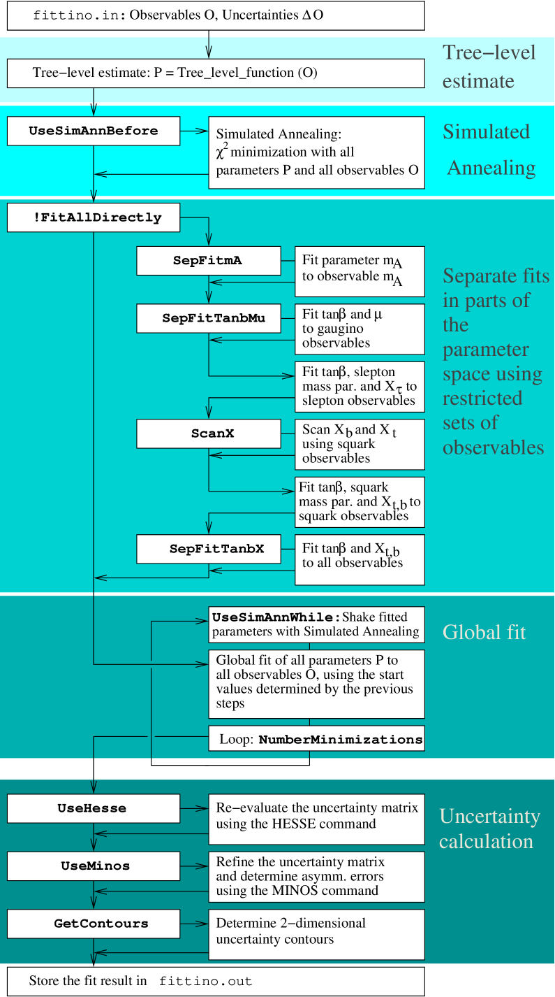
Figure 1: Flow chart of the iterative fit procedure of Fittino. Output and input files are shown in light courier, boolean operations in bold courier and explanations are shown in times.

The iterative procedure of Fittino to determine the start values for the fit, the optimal parameter values and the parameter uncertainties is displayed in Fig. 1. In a first step, the SUSY parameters are estimated using tree-level relations. Then several subsequent subsector fits in parts of the parameter space can be used to improve the tree level estimates before the global fits. This is called the subsector fit method. Alternatively, a Simulated Annealing [10, 11] algorithm can be used to find the minimum. In a third step a global fit of all parameters to all observables is used to fine-tune the optimal parameter values and determine the parameter uncertainties and correlations.

2.2.1 Tree level estimates for the parameters

In order to get the start values for both the subsector fit method and the Simulated Annealing, tree-level relations of the form

$$\mathrm{Observable}=f(\mathrm{Parameters})$$

are inverted to the form

$$\mathrm{Parameter}=f^{\prime}(\mathrm{Observables})$$

and used to estimate the parameters. This is done in the gaugino, the slepton and the squark sectors.

1. $\mu,m_{A},\tan\beta,M_{1},M_{2},M_{3}$ are determined from the gaugino and Higgs sector using formulae from [13, 14]. In order to extract these parameters, information from chargino cross-sections is needed, which enters in form of the chargino mixing angles $\cos 2\phi_{L}$ and $\cos 2\phi_{R}$. These pseudo-observables are just used for the determination of the start values, no use is made of them for the fit. They can be approximately determined from chargino cross-sections at the ILC at different polarisations. If kinematically accessible, $\mbox{$m_{\mathrm{A}}$}_{\mathrm{pole}}$ can be directly measured. The start value of the parameter $\mbox{$m_{\mathrm{A}}$}_{\mathrm{run}}$ is set to $\mbox{$m_{\mathrm{A}}$}_{\mathrm{pole}}$ in this case. For the other parameters, the following individual calculations are performed. For the full form of the relations, see e. g. [7]. Based on the diagonalisation of the chargino mixing matrix the mixing angles $\phi_{L}$ and $\phi_{R}$ can then be used to derive the tree-level estimates of $\mu$, $\tan\beta$ and $M_{2}$:

   $$|\mu| = m_{W}\left(\Sigma+\Delta(\cos 2\phi_{L}+\cos 2\phi_{R})\right)^{\frac{1}{2}}$$ (1)

   $$\tan\beta = \left(\frac{1+\Delta(\cos 2\phi_{R}-\cos 2\phi_{L})}{1-\Delta(\cos 2\phi_{R}-\cos 2\phi_{L})}\right)^{\frac{1}{2}}$$ (2)

   $$M_{2} = m_{W}\left(\Sigma-\Delta(\cos 2\phi_{L}+\cos 2\phi_{R})\right)^{\frac{1}{2}}$$ (3)

   $$\text{sign}(\mu) = -\frac{\Delta^{2}-(\mu^{2}-M_{2}^{2})^{2}-4m_{W}^{2}(\mu^{2}+M_{2}^{2})-4m_{W}^{2}\cos^{2}2\beta}{8m_{W}^{2}M_{2}|\mu|\sin 2\beta}$$ (4)

   $$M_{3} = m_{\tilde{\mathrm{g}}}$$ (5)

   using

   $$\Sigma = \frac{m^{2}_{\chi^{\pm}_{2}}+m^{2}_{\chi^{\pm}_{1}}}{2m^{2}_{W}}-1$$ (6)

   $$\Delta = \frac{m^{2}_{\chi^{\pm}_{2}}-m^{2}_{\chi^{\pm}_{1}}}{4m^{2}_{W}}$$ (7)

   After these parameters have been determined at tree-level, a tree-level estimate of $M_{1}$ can be calculated from the neutralino mass matrix eigenvalues. They depend on $\mu,\mbox{$\tan\beta$},M_{2}$ and $M_{1}$. The first three of these parameters have been determined already in the first step. Thus the neutralino system can be used to finally determine $M_{1}$. In fact, the neutralino system is the only sector where $M_{1}$ can be measured directly. The characteristic equation of the neutralino mass matrix then is used to determine $M_{1}$ [14].

2. $X_{\mathrm{t}},X_{\mathrm{b}},M_{Q},M_{U},M_{D}$ are determined from the squark sector masses, using formulae from [15]. The trilinear coupling parameters $A$ are set to zero for the determination of the squark mass parameters. $X_{\mathrm{t}}=A_{\mathrm{t}}-\mu/\mbox{$\tan\beta$}$ and $X_{\mathrm{b}}=A_{\mathrm{b}}-\mu\mbox{$\tan\beta$}$ are chosen as fit parameters instead of $A$ because their correlation with $\tan\beta$ is reduced. After $\tan\beta$ and $\mu$ have been determined in the previous step, the following tree-level relations can be used. As an example, only the third generation is shown explicitly.

   $$M_{\tilde{\mathrm{t}}_{L}} = -\mbox{$m_{\mathrm{Z}}$}^{2}\cos 2\beta(\frac{1}{2}-\frac{2}{3}\sin^{2}\theta_{W})-m_{\mathrm{t}}^{2}+\frac{1}{2}(m^{2}_{\tilde{\mathrm{t}}_{1}}+m^{2}_{\tilde{\mathrm{t}}_{2}})$$ (8)

   $$= \mbox{$m_{\mathrm{Z}}$}^{2}\cos 2\beta(\frac{1}{2}-\frac{1}{3}\sin^{2}\theta_{W})-m_{\mathrm{b}}^{2}+\frac{1}{2}(m^{2}_{\tilde{\mathrm{b}}_{1}}+m^{2}_{\tilde{\mathrm{b}}_{2}})$$ (9)

   $$M_{\tilde{\mathrm{t}}_{R}} = -\mbox{$m_{\mathrm{Z}}$}^{2}\cos 2\beta\frac{2}{3}\sin^{2}\theta_{W}-m_{\mathrm{t}}^{2}+\frac{1}{2}(m^{2}_{\tilde{\mathrm{t}}_{1}}+m^{2}_{\tilde{\mathrm{t}}_{2}})$$ (10)

   $$M_{\tilde{\mathrm{b}}_{R}} = \mbox{$m_{\mathrm{Z}}$}^{2}\cos 2\beta\frac{1}{3}\sin^{2}\theta_{W}-m_{\mathrm{b}}^{2}+\frac{1}{2}(m^{2}_{\tilde{\mathrm{b}}_{1}}+m^{2}_{\tilde{\mathrm{b}}_{2}})$$ (11)

   $$X_{\mathrm{t}} = -\mu/\mbox{$\tan\beta$}$$ (12)

   $$X_{\mathrm{b}} = -\mu\mbox{$\tan\beta$}$$ (13)

   The parameters of the other generations can be obtained analogously. The initial determination of $X_{\mathrm{t}}$ and $X_{\mathrm{b}}$ is only very rough and therefore refined in an additional step, which is explained below.

3. $X_{\tau},M_{L},M_{E}$ are determined from the slepton sector masses, using formulae from [15]. Their calculation is analogous to the calculation of the squark parameters in the previous item. The determination of $X_{\tau}$ is refined later as explained below.

In order to estimate the uncertainty of this determination of the parameters from tree-level formulae, the calculation is repeated 10 000 times with observables randomly smeared within their uncertainties according to a Gaussian probability distribution. The starting value of the fit is the mean of the distribution of each parameter. From the variance of the calculated parameter distribution the initial uncertainty is estimated.

2.2.2 Finding the optimal parameter values

A global $\chi^{2}$ fit of a large number of MSSM parameters with starting values derived from tree-level relations will most likely fail to find the global $\chi^{2}$ minimum, since the parameter space contains many local minima. Therefore the tree-level estimates have to be improved before the global fit. This can be done by using knowledge about the dependencies of sets of individual parameters on sets of individual observables. This is done in the fast subsector fit method. However, also in this case some local minima can be too deep to allow MINUIT to escape from them. Therefore the slower but very stable Simulated Annealing algorithm has been implemented alternatively.

Subsector Fit Method

Since the possibility of mixing in the third generation has been neglected in the calculation of the tree-level estimates, the parameters $X_{\mathrm{t}},X_{\mathrm{b}},X_{\tau}$ are only roughly initialised. A global fit with these starting values would most likely not converge. Therefore next the estimates from the slepton sector are improved by fitting only the slepton parameters $X_{\tau},M_{L},M_{E}$ to the observables from the slepton sector, i. e. slepton masses, widths and cross-sections. Observables not directly related to the slepton sector can degrade the fit result, since parameters of other sectors are likely to be still wrong. In such a case a parameter of the slepton sector will be pulled into a wrong direction, in order to compensate for the wrong parameters of other sectors. All parameters not from the slepton sector are fixed to their estimated tree-level values. In this fit with reduced number of dimensions MINUIT can handle the correlations among the parameter better than in a global fit with all parameters free.

Then the third generation squark parameters are improved by only fitting $X_{\mathrm{t}},X_{\mathrm{b}},M_{Q},M_{U},M_{D}$ to the observables of the squark sector, masses, widths and cross-sections. All other parameters are fixed to their previous values.

After this step the correlations among $\tan\beta$ and the third generation slepton and squark parameters are still not optimally modelled. Therefore another intermediate step is introduced, where $\tan\beta,X_{\mathrm{t}},X_{\mathrm{b}},X_{\tau}$ and $M_{\tilde{\mathrm{t}}_{L,R}}$ are fitted to all observables and all other parameters are fixed to their present values.

The subsector fit method does not yield a parameter set which corresponds to the global minimum of the $\chi^{2}$. But starting from the result of the subsector fit method, the subsequent global fit (see Section 2.2.3) is able to converge to the global minimum.

Simulated Annealing

In the method of Simulated Annealing, the $\chi^{2}$ surface in the MSSM parameter space is treated as a potential. A temperature $t$ is defined, which according to a Boltzmann-distribution sets the probability of a movement in the parameter space which corresponds to an upward movement in the potential, i.e. which results in a larger $\chi^{2}$ than the parameter setting in the step before. In the process of Simulated Annealing, the temperature is reduced step by step. This ensures that large movements over high potential barriers are possible in the early stages of the annealing process, in order to escape from local minima. Later, the temperature is reduced and the parameter setting is thus forced into areas with low $\chi^{2}$. The individual steps of the algorithm work as follows:

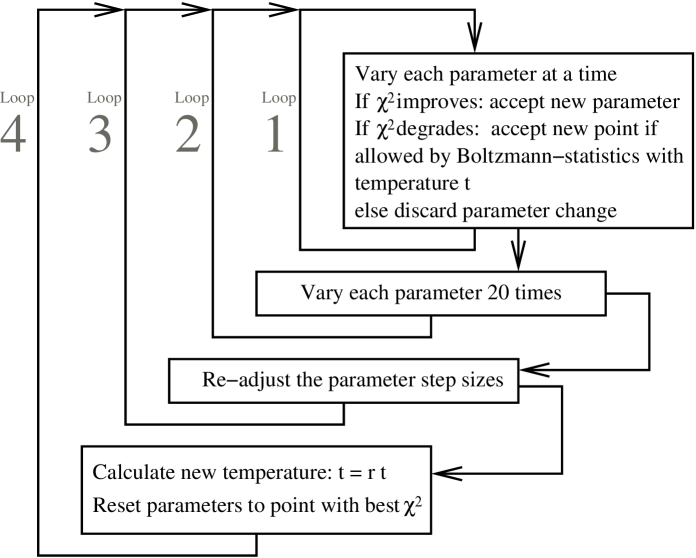
Figure 2: Structure of the Simulated Annealing algorithm. The four different loops are indicated by the grey numbers.

First, the initial temperature $t_{0}$ is determined by varying each parameter 10 times randomly within its estimated uncertainty. The estimated uncertainty is determined from the tree-level estimates. Then half of the standard deviation

$$\sigma_{\chi^{2}}=\sqrt{\langle(\chi^{2})^{2}\rangle-\langle\chi^{2}\rangle^{2}}$$

of the $\chi^{2}$ values obtained is taken as initial temperature. This choice is large enough to allow the algorithm to scan large parts of the parameter space and to escape from local minima.

The core of the Simulated Annealing algorithm is schematically shown in Fig. 2. In the innermost loop (loop No. 1 in Fig. 2), each parameter $P_{i}$ is varied at a time by a random variation within the estimated uncertainties of each parameter $\Delta P_{i}$. These uncertainties are initially taken from the tree-level estimates and later refined for each parameter individually, as described below. After the parameter variation, the $\chi^{2}$ at the new parameter setting is evaluated. If the new value $\chi^{2}_{i}$ lies below $\chi^{2}_{i-1}$, where $\chi^{2}_{i-1}$ is the $\chi^{2}$ value of the last accepted parameter set, the new parameter value is accepted and the next parameter is varied. If the new value $\chi^{2}_{i}$ is the best $\chi^{2}$ value achieved so far, $\chi^{2}_{i}$ and the accompanying parameter set are stored. If $\chi^{2}_{i}>\chi^{2}_{i-1}$, then the new point is accepted on the basis of a Boltzmann distribution: If a random number $p\,\epsilon\,[0,1]$ fulfils

$$p<e^{-\frac{\chi^{2}_{i}-\chi^{2}_{i-1}}{t}},$$

then the new parameter value is accepted despite yielding a worse fit than the previous parameter set. This ensures that the algorithm is able to escape from local minima.

In loop 2 the variation of each parameter at a time is repeated 20 times. On each variation the number of accepted ($n_{\mathrm{acc}}$) and rejected ($n_{\mathrm{tot}}-n_{\mathrm{acc}}$) parameter choices is counted for each parameter. After loop 2, the estimated parameter uncertainty $\Delta P_{i}$ is iteratively re-adjusted such that $n_{\mathrm{acc}}/n_{\mathrm{tot}}$ lies in the range of 0.4 to 0.6. This is achieved by the transformation

$$\Delta P_{i}>0.6 : \Delta P^{\mathrm{new}}_{i}=\Delta P^{\mathrm{old}}_{i}\left(2\frac{\frac{n_{\mathrm{acc}}}{n_{\mathrm{tot}}}-0.6}{0.4}+1\right),$$

$$\Delta P_{i}<0.4 : \Delta P^{\mathrm{new}}_{i}=\frac{\Delta P^{\mathrm{old}}_{i}}{\left(2\frac{0.4-\frac{n_{\mathrm{acc}}}{n_{\mathrm{tot}}}}{0.4}+1\right)}.$$

In loop 3 this re-adjustment of the parameter uncertainties is repeated $3n$ times for $n$ parameters, but at least 60 times in case $n<20$. The re-adjustment of the parameters variation ensures that for each temperature $t$ the random parameter variation tests a parameter range with values of $\chi^{2}_{1}-\chi^{2}_{i-1}\approx t$.

After loop 3 is completed, the temperature is reduced by the multiplication with a factor $r$, which is constant during the algorithm. At the same time, the parameter values for the next iteration are set to the parameter set with the lowest $\chi^{2}$ found so far. The whole procedure is repeated until one of the two exit criteria are met. Either, the allowed number of calls to the theory code is reached, or the variation of the $\chi^{2}$ value within loop 3 is smaller than the variation within the last four lowest $\chi^{2}$ values found, and the variation of all values is smaller than 0.0001. In each case the Simulated Annealing algorithm exits with the parameter set which yields the best $\chi^{2}$ found so far.

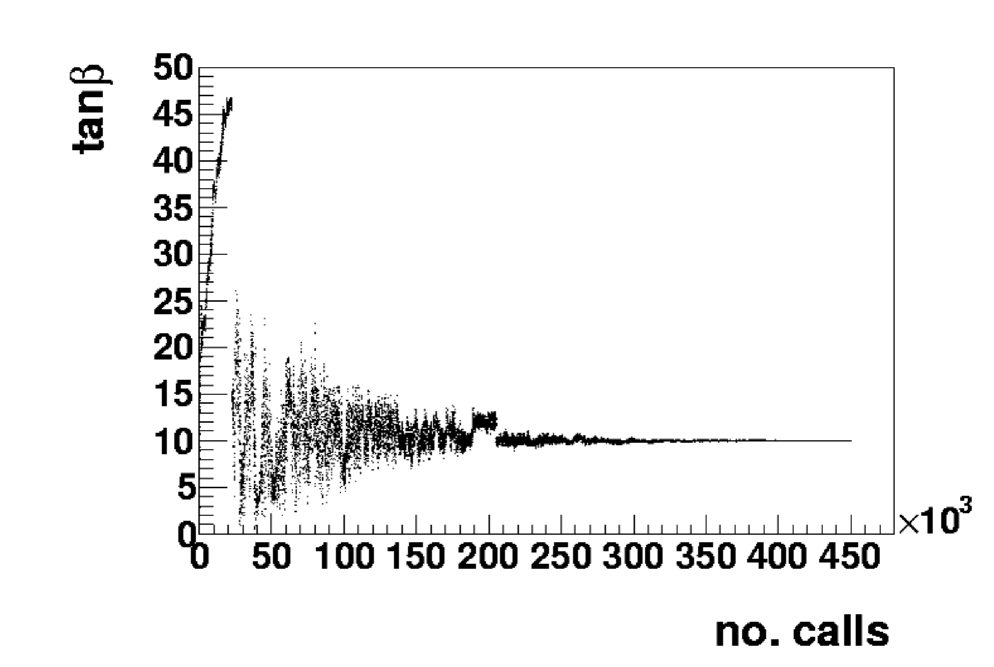
(a)

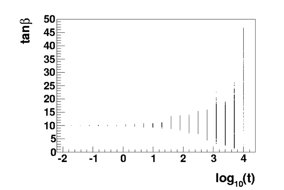
(b)

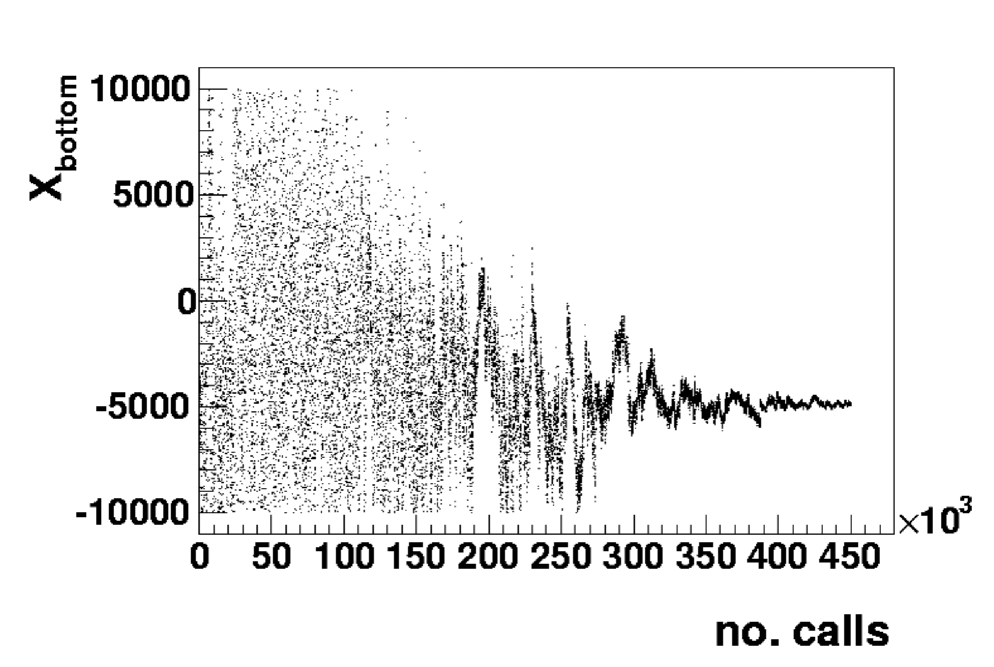
(c)

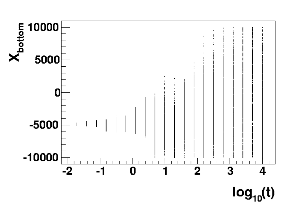
(d)

Figure 3: The parameter determination using Simulated Annealing in a fit with 19 parameters in the SPS1a’ [3] scenario. In (a), the tested parameter values of $\tan\beta$ are shown versus the number of calls to SPheno. In (b) the same evolution is shown against $\log_{10}(t)$, where $t$ is the temperature of the Simulated Annealing. In (c) and (d), the same projections are shown for $X_{\mathrm{bottom}}$, which in contrast to $\tan\beta$ is only weakly constrained by the measurements.

The Simulated Annealing algorithm has been tested on fits with 20 free parameters in the scenarios SPS1a’ [3] and SPS7 [16]. In each case, the convergence to the true minimum of the $\chi^{2}$ is good and very stable. However, while being very robust, this algorithm is considerably slower than the subsector fit method. In Fig. 3, some distributions illustrating the behaviour of the Simulated Annealing in the SPS1a’ scenario are shown. In Fig. 3 (a), the variation of $\tan\beta$ with the number of calls to SPheno is shown. In the beginning, a large range of $\tan\beta$ is scanned. For lower $t$ at a larger number of calls, the parameter variation $\Delta\mbox{$\tan\beta$}$ is reduced along with $t$ and convergence is achieved. Thus Simulated Annealing is very effectively coarsely scanning a large parameter space at high $t$, while it is also finely testing the area close to the $\chi^{2}$ minimum. The same evolution is shown in (b) against the temperature $t$. In (c) and (d), the same evolution is shown for the bottom-squark mixing parameter $X_{\mathrm{bottom}}$, which is much weaker constrained that $\tan\beta$ and therefore takes longer to converge.

Simulated Annealing is a robust and reliable algorithm, which is better capable of escaping from local minima than the subsector fit method. Also it is much less dependent on the starting values obtained from the tree-level estimate. However, it is more computing time consuming, since a high initial temperature is necessary to overcome the local minima near the tree-level estimates of the parameters and find the true minimum.

2.2.3 Determining the parameter uncertainties and correlations

After the search for the optimal parameters, all parameters are released and a global fit is done, using the method MINIMIZE in MINUIT. In case the subsector fit method has been used for the improvement of the tree-level estimates of the parameters, this step is also necessary to find the optimal parameters, which are generally not yet perfectly determined after the subsector fits. If Simulated Annealing with a sufficient number of iterations is used, then the optimal parameters after Simulated Annealing are generally very close to the true parameter values.

If the global fit converges, a MINOS error analysis is performed, yielding symmetrical and asymmetrical uncertainties, the full correlation matrix and 2D fit contours.

3 The Fittino Steering File

Fittino is controlled using an ASCII input file whose name is passed to Fittino as parameter. If none is given, fittino.in is assumed. An example for this file is given in Section A.1. The user can specify the observables, their values and uncertainties, their correlations, the fitted and fixed parameters and universalities among generations. Flags can be used to control the general behaviour of Fittino. A list of the available commands is given in Tables 1 and 2. In the following, the syntax of the commands is explained.

Table 1: Commands in the Fittino steering file. All commands given in this table set the input observables and the parameters used by Fittino. The full form of the commands is given in the text. The correlations must be specifyed after all observables. The steering flags can be found in Tab. 2.

Command	Explanation
Keys before any line
#	Comment line
nofit	The observable after nofit is not used in the fit
Observables
mass<name>	Mass of the particle <name>, see Tab. 3
edge	Position of an edge in a mass spectrum
sigma	cross section of a process
BR	Branching fraction
width	Total width of a particle
limit	Limits on particle masses
LEObs	Low energy observable
sin2thetaW	The value of $\sin^{2}\theta_{W}$
cos2phiL	The value of $\cos 2\phi_{L}$
cos2phiR	The value of $\cos 2\phi_{R}$
xsbr	Product of cross-sections and branching fractions
brratio	Ratio of two branching fractions
brsum	Sum of branching fractions
Correlations
correlationCoefficient	Correlation coefficient of two observables
Parameters
fitParameter	Name and eventually value of a fitted parameter
fixParameter	Name and value of a fixed parameter
universality	Specifies which parameters are unified

Table 2: Flags in the Fittino steering file. The commands given here determine the fit strategies and outputs of Fittino. The full form of the commands is given in the text. The correlations must be specified after all observables. The other commands used for the Fittino input can be found in Tab. 1.

Flags
FitModel	Model type, such as MSSM, mSUGRA, etc.
LoopCorrections	Use full loop corrections as provided by SUSY calculator
ISR	Switch on ISR
UseGivenStartValues	Start from parameter values in fitParameter
FitAllDirectly	Fit all parameters at once
CalcPullDist	Calculate pull distributions
CalcIndChisqContr	Calculate individual $\Delta\chi^{2}$ contributions
BoundsOnX	Set bounds on $X_{\tau}$, $X_{\mathrm{t}}$ and $X_{\mathrm{b}}$
ScanX	Scan $X_{\mathrm{t}}$ and $X_{\mathrm{b}}$ before fitting
SepFitTanbX	Perform separate fit of $\tan\beta$, $M_{\tilde{\mathrm{t}}_{R}}$, $M_{\tilde{\mathrm{t}}_{L}}$, $X_{\mathrm{t}}$ and $X_{\mathrm{b}}$
SepFitTanbMu	Perform separate fit of $\tan\beta$ and $\mu$
SepFitmA	Perform separate fit of $\mbox{$m_{\mathrm{A}}$}_{\mathrm{run}}$ to $\mbox{$m_{\mathrm{A}}$}_{\mathrm{pole}}$
Calculator	Specify calculator for theory predictions
UseMinos	Use MINOS error calculation
UseHesse	Use HESSE error matrix calculation
NumberOfMinimizations	Number of minimisation steps
ErrDef	The error definition used in MINOS
NumberPulls	Number of pull fits
GetContours	Determine 2D uncertainty contours
UseSimAnnBefore	Use Simulated Annealing algorithm directly after
	tree-level estimation
UseSimAnnWhile	Use Simulated Annealing algorithm between global
	fits for NumberOfMinimizations $>1$
TempRedSimAnn	Temperature reduction factor in Simulated Annealing
MaxCallsSimAnn	Maximum number of calls in Simulated Annealing
InitTempSimAnn	Initial temperature of the Simulated Annealing
Verbose	Verbose mode
ScanParameters	Scan one- or two-dimensional parameter space and write
	$\chi^{2}$-surface to ROOT file
scanParameter	Specify parameters to scan, the scan range and the
	number of scan steps for ScanParameters
PerformFit	Controls whether fit is performed or not
RandomGeneratorSeed	Seed for the random number generator
MaxCalculatorTime	Maximal allowed time for the SUSY calculator code

Keys

The commands in this group act on the contents of the line after the key. Available keys are:

• #
  Comment line. Everything after # is ignored by Fittino.

• nofit <observable> <value> +- <uncertainty>
  This key can be used to specify observables which shall only be used in the step of the initialisation of parameters using tree-level relations. Typical examples are the chargino mixing angles $\cos 2\phi_{L}$ and $\cos 2\phi_{R}$.

Observables

The commands in this group specify the measured (or simulated) observables and their values and uncertainties. The following types of observables are available:

• mass<name> <value> +- <uncertainty> [ +- <theo_uncertainty> ]
  Specifies the mass of the particle <name>. All available particles are listed in Tab. 3. If no uncertainty is given, the particle mass is not used in the $\chi^{2}$ of the fit. If more than one uncertainty is given, the uncertainties are added in quadrature. This is useful in case large theoretical uncertainties on the predicted particle mass exist. For the time being it is assumed that treating the theoretical uncertainties as uncorrelated with the experimental error and a Gaussian probability distribution is reasonable.

  If no unit is given in <value> and <uncertainty>, they are assumed to be given in GeV. Other supported units range from eV to EeV.

  Table 3: Particles known to Fittino. The following particles can be used after mass, sigma, BR and width. Antiparticles are identified by ~ after the particle name.

  Particle Name	Explanation	Particle Name	Explanation
  W	W boson	SelectronL	$\tilde{\mathrm{e}}_{L}$ selectron
  Z	Z boson	SelectronR	$\tilde{\mathrm{e}}_{R}$ selectron
  gamma	$\gamma$	SnueL	$\tilde{\nu}_{\mathrm{e}_{L}}$ electron sneutrino
  gluon	gluon	SmuL	$\tilde{\mu}_{L}$ smuon
  Up	u quark	SmuR	$\tilde{\mu}_{R}$ smuon
  Down	d quark	SnumuL	$\tilde{\nu}_{\mu_{L}}$ muon sneutrino
  Charm	c quark	Stau1	$\tilde{\tau}_{L}$ stau
  Strange	s quark	Stau2	$\tilde{\tau}_{R}$ stau
  Top	t quark	Snutau1	$\tilde{\nu}_{\tau_{1}}$ tau sneutrino
  Bottom	b quark	Gluino	$\tilde{\mathrm{g}}$ gluino
  Electron	electron	Neutralino1	$\chi^{0}_{1}$ neutralino
  Nue	electron neutrino $\nu_{\mathrm{e}}$	Neutralino2	$\chi^{0}_{2}$ neutralino
  Mu	muon	Neutralino3	$\chi^{0}_{3}$ neutralino
  Numu	muon neutrino $\nu_{\mu}$	Neutralino4	$\chi^{0}_{4}$ neutralino
  Tau	tau	Chargino1	$\chi^{+}_{1}$ chargino
  Nutau	tau neutrino $\nu_{\tau}$	Chargino2	$\chi^{+}_{2}$ chargino
  h0	h CP-even Higgs boson
  A0	A CP-odd Higgs boson
  H0	H CP-even Higgs boson
  Hplus	H± charged Higgs boson
  SdownL	$\tilde{\mathrm{d}}_{L}$ squark
  SdownR	$\tilde{\mathrm{d}}_{R}$ squark
  SupL	$\tilde{\mathrm{u}}_{L}$ squark
  SupR	$\tilde{\mathrm{u}}_{R}$ squark
  SstrangeL	$\tilde{\mathrm{s}}_{L}$ squark
  SstrangeR	$\tilde{\mathrm{s}}_{R}$ squark
  ScharmL	$\tilde{\mathrm{c}}_{L}$ squark
  ScharmR	$\tilde{\mathrm{c}}_{R}$ squark
  Sbottom1	$\tilde{\mathrm{b}}_{1}$ squark
  Sbottom2	$\tilde{\mathrm{b}}_{2}$ squark
  Stop1	$\tilde{\mathrm{t}}_{1}$ squark
  Stop2	$\tilde{\mathrm{t}}_{2}$ squark

• edge <type> <mass1> <mass2> [more masses] <value> +-
<uncertainties> alias <alias>
  Specifies the edge in a mass spectrum. Since SUSY particles tend to decay in cascade decays, the masses of intermediate particles can often be reconstructed from edges in mass spectra. If the edges are transformed into masses before the fit is made, the correlations among the reconstructed masses from one spectrum have to be specified using correlationCoefficient. The command edge offers the simpler and more straightforward possibility to use the edge positions in the mass spectra directly in the fit. Momentarily, the following types <type> are available:
  1 $m_{1}+m_{2}$ 2 $|m_{1}-m_{2}|$ 3 $\frac{(m_{2}^{2}-m_{3}^{2})(m_{3}^{2}-m_{1}^{2})}{m_{3}^{2}}$ [17] 4 $\frac{(m_{4}^{2}-m_{2}^{2})(m_{3}^{2}-m_{1}^{2})}{m_{3}^{2}}$ [17] 5 $[(m_{4}^{2}+m_{2}^{2})(m_{2}^{2}-m_{3}^{2})(m_{3}^{2}-m_{1}^{2})$ $-(m_{4}^{2}-m_{2}^{2})\sqrt{(m_{2}^{2}+m_{3}^{2})^{2}(m_{3}^{2}+m_{1}^{2})^{2}-16m_{2}^{2}m_{3}^{4}m_{1}^{2}}$ $+2m_{3}^{2}(m_{4}^{2}-m_{2}^{2})(m_{2}^{2}-m_{1}^{2})]/(4m_{3}^{2}m_{2}^{2})$ [17]
  The list of formulae can be easily extended. Here and in most of the following commands <alias> is an integer number which can be used to unambigously identify the input if it is used in other commands, such as correlationCoefficient.

• sigma ( <initial_state> -> <final_state_particles>,<Ecms>,<polarisation1>,
<polarisation2>) [ <value> +- <uncertainties> ] alias <alias>
  Specifies the cross section of a given process <initial_state> -> <final_state_particles>, where <final_state_particles> is a list of particle names. Antiparticles are specified by <particle>~. Momentarily only ${\mathrm{e}}^{+}{\mathrm{e}}^{-}$ processes are implemented, identified by <initial_state>=ee. The centre-of-mass energy (if no unit is given, GeV is assumed) is given by <Ecms>, the polarisation of the incoming particles are given by <polarisation1> and <polarisation2>. If no unit of the cross-section and the uncertainty is given, they are assumed to be given in fb. The integer number <alias> identifies the cross-section in the correlationCoefficient commands. No value and uncertainty must be given if the cross section is not used as an observable on its own but within xsbr instead.

• BR ( <decaying_particle> -> <decay_products> ) [ <value>
+- <uncertainties> ] alias <alias>
  Specifies the branching fraction of a given particle <decaying_particle> into the decay products <decay_products>. The integer number <alias> identifies the branching fraction in the correlationCoefficient commands. No value and uncertainty must be given if the branching fraction is not used as an observable on its own but within brsum, xsbr or brratio instead.

• brsum ( br_<alias1> br_<alias2> [...] ) <value>
+- <uncertainties> alias <alias>
  Specifies the sum of several branching fractions, which all have to be defined with a unique alias number before. No value and uncertainty must be given if the sum of branching fractions is not used as an observable on its own but within xsbr or brratio instead.

• width <particle> <value> +- <uncertainties> alias <alias>
  Specifies the total width of the particle <particle>. If no unit is given in <value> and <uncertainty>, they are assumed to be given in GeV.

• limit mass<name> <$|$> <limit>
  Allows the user to specify upper or lower mass limits of yet undiscovered SUSY particles. The limit is used in the calculation of the $\chi^{2}$ of the fit in the following way: If the predicted mass is in agreement with the limit, the contribution of this observable to the total $\chi^{2}$ is zero. If the limit is violated by the predicted mass $m_{p}$, the $\chi^{2}$ contribution is ((<limit>$-m_{p}$)/(<limit>/10))², i. e. a 10 % violation of the limit adds 1 to the $\chi^{2}$ of the fit.

• LEObs ( <name> ) <value> +- <uncertainties> alias <alias>
  Low-energy precision observable. In Fittino 1.1 the following observables names are implemented:

  • bsg: BR($b\rightarrow s\gamma$)

  • gmin2: $(g-2)_{\mu}$

  • drho: $\Delta\rho$

• xsbr ( sigma_<alias1> [sigma_<alias2> [...]] br_<alias3>
[br_<alias4> [...]] ) <value> +- <uncertainties> alias <alias>
  Product of an arbitrary number of cross sections and branching fractions. This command must be used in the input file after all cross sections and branching fractions have been defined. The product of cross sections and branching fractions is then specified by the alias numbers of the individual observables. These are automatically not used in the fit anymore. Therefore the actual values entered for the individual observables are irrelevant, if they are used in xsbr. Instead of br_<alias> also brsum_<alias> can be used.

• brratio ( br_<alias1> br_<alias2> ) <value> +- <uncertainties> alias <alias>
  Ratio of two branching fractions: br_<alias1>/br_<alias2>. Also here the individual branching fractions must be defined before their use in brratio and are not used in the fit. Instead of br_<alias> also brsum_<alias> can be used.

• Other observables dedicated for special cases are

  • sin2thetaW <value> +- <uncertainties>
    Specifies the value of $\sin^{2}\theta_{W}$

  • cos2phiR <value> +- <uncertainties>
    

  • cos2phiL <value> +- <uncertainties>
    Specify the values of the chargino mixing angles, used for initialisation.

Correlations among observables

After all observables have been specified, the following command can be used to specify the correlation among observables.

• correlationCoefficient <observable1> <observable2> <value>
  If the observables are masses, they are identified by mass<name>. All other observables are identified by their alias number, such as sigma_<alias>.

Parameters

Fittino can fit any combination of the MSSM-24 and SM parameters given in Tab. 4 to the observables given in the input file. As alternatives to MSSM-24, high-scale parameters of the mSUGRA, GMSB and AMSB models can be determined. The following commands can be used to specify the parameters that are fitted to the observables and the parameters which are kept fixed.

Table 4: MSSM parameters known to Fittino. The following parameters can be used with fitParameter, fixParameter and universality.

Parameter Name	Explanation
TanBeta	Ratio of Higgs vacuum expectation values
Mu	$\mu$ parameter, controls Higgsino mixing
Xtau	Tau mixing parameter
Xtop	Top mixing parameter
Xbottom	Bottom mixing parameter
MSelectronR	Right scalar electron mass parameter
MSmuR	Right scalar muon mass parameter
MStauR	Right scalar tau mass parameter
MSelectronL	Left 1st. gen. scalar lepton mass parameter
MSmuL	Left 2nd. gen. scalar lepton mass parameter
MStauL	Left 3rd. gen. scalar lepton mass parameter
MSdownR	Right scalar down mass parameter
MSstrangeR	Right scalar strange mass parameter
MSbottomR	Right scalar bottom mass parameter
MSupR	Right scalar up mass parameter
MScharmR	Right scalar charm mass parameter
MStopR	Right scalar top mass parameter
MSupL	Left 1st. gen. scalar quark mass parameter
MScharmL	Left 2nd. gen. scalar quark mass parameter
MStopL	Left 3rd. gen. scalar quark mass parameter
M1	$U(1)_{Y}$ gaugino (Bino) mass parameter
M2	$SU(2)_{L}$ gaugino (Wino) mass parameter
M3	$SU(3)_{C}$ gaugino (gluino) mass parameter
massA0	Pseudoscalar Higgs mass
massW	W boson mass
massZ	Z boson mass
massTop	Top quark mass $m_{\mathrm{t}}(m_{\mathrm{t}})$
massBottom	Bottom quark mass $m_{\mathrm{b}}(m_{\mathrm{b}})$
massCharm	Charm quark mass $m_{\mathrm{c}}(m_{\mathrm{c}})$

• fitParameter <parameter> [ <value> [ +- <uncertainty>] ]
  Specifies one of the parameters that should be fitted. The names which are available for <parameter> are listed in Tab. 4. If a value <value> is given, then using FitAllDirectly it is possible to specify that <value> should be the initial value of the parameter in the fit. If additionally an uncertainty is given, then this can be used in the pull distribution calculation with CalcPullDist or CalcIndChisqContr. If no unit for <value> is given for a dimension-full parameter, then it is assumed to be given in GeV.

• fixParameter <parameter> <value>
  Specifies a parameter kept fixed during the fit.

• universality <parameter1> <parameter2> [...]
  Specifies that <parameter2> (and possible other following parameters) should not be fitted on its own, but that it should be set to the value of <parameter1> during the fit. This is useful if unification among generations shall be assumed.

Flags

The following flags can be used to control the behaviour of Fittino during the fit and to specify what operations Fittino should perform.

• fitModel <model>
  SUSY model under study. The default value is MSSM, with the 24 low-scale SUSY Lagrangian parameters from Tab. 4 as parameters. If fitModel is mSUGRA, the mSUGRA parameters TanBeta, M0, M12 and A0 can be fitted using fitParameter, and SignMu can be fixed with fixParameter. Thus the high-scale parameters can be fitted directly to the observables. Correspondingly GMSB and AMSB parameters can be fitted/fixed, if fitModel is set to GMSB and to AMSB respectively. In these cases the parameter names are TanBeta, Lambda, Mmess, cGrav, N5 and SignMu in case of GMSB and TanBeta, M0, M32 and SignMu for AMSB models.

• LoopCorrections on|off
  If LoopCorrections is off, then no fit is performed but just the tree-level estimates of the parameters are calculated. By default it is on.

• ISR on|off
  Switches ISR corrections in the cross-section calculations on or off. By default it is on.

• UseGivenStartValues on|off
  If UseGivenStartValues is on, then the start values of the parameters in the fit are not determined from tree-level estimates, but from the values given in fitParameter. By default it is off.

• FitAllDirectly on|off
  If FitAllDirectly is on, then the initial fits of subsets of the parameter space (as described above in Section 2) are omitted. By default it is off.

• CalcPullDist on|off
  If CalcPullDist is on, then pull distributions for all parameters specified with fitParameter are calculated. It is necessary that each parameter is given with its value and uncertainty. The pull distribution is then calculated with respect to the parameter value and the width is compared with the parameter uncertainty. For each parameter, a ROOT [18] histogram is created in the output file PullDistributions.root. Additionally, a ROOT tree with all fitted parameters and the corresponding $\chi^{2}$ values is created, which allows for the extraction of the parameter correlations. The number of fits per Fittino run can be specified using the command NumberPulls. By default CalcPullDist is off. This command is very useful to test the fitted parameters and their uncertainties calculated in a previous run of Fittino.

• CalcIndChisqContr on|off
  If CalcIndChisqContr is on, for each parameter specified with fitParameter the individual contribution of each observable to the $\Delta\chi^{2}$ of the fit is calculated, if the parameter is varied by $\pm 1\,\sigma$. It is necessary that each parameter is given with its value and uncertainty. The parameter is varied once by $+1\,\sigma$ and once by $-1\,\sigma$. The resulting total $\Delta\chi^{2}$ and the individual $\Delta\chi^{2}_{i}$ of each observable $O_{i}$ are averaged. The total $\Delta\chi^{2}$ indicates the correlation of the parameter with all other parameters. If the parameters are not too strongly correlated, the individual $\Delta\chi^{2}_{i}$ provide a measure for the contribution of observable $O_{i}$ to the determination of the parameter. The output is given in the file fittino_individual_chisq_contr.out. By default, CalcIndChisqContr is off.

• BoundsOnX on|off
  If BoundsOnX is on, then the parameters $X_{\tau}$, $X_{\mathrm{t}}$ and $X_{\mathrm{b}}$ are bounded between Xscanlow$<X<$Xscanhigh. By default BoundsOnX is on.

• SepFitmA on|off
  If SepFitmA is on, a separate fit of $m_{\mathrm{A}_{\mathrm{run}}}$ to $m_{\mathrm{A}_{\mathrm{pole}}}$ is performed, in order to improve the start value of the parameter $m_{\mathrm{A}_{\mathrm{run}}}$. This is necessary in some scenarios, where the difference between $m_{\mathrm{A}_{\mathrm{pole}}}$ (which is used as a tree-level estimate of $m_{\mathrm{A}_{\mathrm{run}}}$) and $m_{\mathrm{A}_{\mathrm{run}}}$ is large and correlations of $m_{\mathrm{A}_{\mathrm{run}}}$ are strong. By default SepFitmA is off.

• SepFitTanbMu on|off
  If SepFitTanbMu is on, a separate fit of $\tan\beta$ and $\mu$ is performed before the main fit and directly after the separate fit of $m_{\mathrm{A}_{\mathrm{run}}}$ to $m_{\mathrm{A}_{\mathrm{pole}}}$. Only gaugino observables are used. By default SepFitTanbMu is off.

• ScanX on|off
  If ScanX is on, then the parameters $X_{\mathrm{t}}$ and $X_{\mathrm{b}}$ are individually scanned in the range $-6000<X<2000$ before the main fit and before the separate fit of the squark sector. This helps to avoid local minima which typically occur at parameter values with the wrong sign. By default ScanX is on.

• SepFitTanbX on|off
  If SepFitTanbX is on, a separate fit of $\tan\beta$, $M_{\tilde{\mathrm{t}}_{R}}$, $M_{\tilde{\mathrm{t}}_{L}}$, $X_{\mathrm{t}}$ and $X_{\mathrm{b}}$ is performed before the main fit and after the separate fit of the squark sector. Only squark sector observables are used. By default SepFitTanbX is on.

• Calculator <calculator_name> <path>
  Specifies the tool for the calculation of the theory predictions. <path> specifies the location of the calculator executable. Currently SPheno is implemented, but also any other tool capable of input and output according to the SUSY Les Houches Accord [6] can be easily interfaced with Fittino.

• UseMinos on|off
  If UseMinos is on, then MINOS is used to perform a detailed uncertainty analysis after MINIMIZE converged. UseMinos implies automatically that UseHesse is on (see below). Since this can take very long (order of several days on a PIII 1.3GHz in a typical fit of the full MSSM spectrum), this option is off by default.

• UseHesse on|off
  If UseHesse is on, then the HESSE function in MINUIT is used to perform a detailed error matrix calculation after MINIMIZE converged, assuming parabolic errors. By default, UseHesse is off.

• GetContours on|off
  If GetContours is on, after MINOS the two-dimensional uncertainty contours of all combinations of two parameters are calculated and stored in the output files FitContours.root (fit contours with an error definition of $\Delta\chi^{2}=1$ (thus the resulting two-dimensional surface will not be the two-dimensional 68 % region) and all parameters free) and FitContours_2params_free.root (just two parameters free per contour). Since this can take very long (order of several days to several weeks in a typical fit of the full MSSM spectrum), this option is off by default.

• UseSimAnnBefore on|off
  If UseSimAnnBefore is on, a Simulated Annealing algorithm is used directly after the tree-level estimates of the parameters. Typically this algorithm is very robust and finds the global minimum of the $\chi^{2}$ reliably. The maximum number of calls to the theory code in the Simulated Annealing process is regulated using MaxCallsSimAnn, which by default is 300 000. The temperature reduction can be set using TempRedSimAnn, which by default is 0.4. The history of the Simulated Annealing process is recorded in a ROOT ntuple the file SimAnnNtupFile.root. By default, UseSimAnnBefore is off.

• UseSimAnnWhile on|off
  If UseSimAnnWhile is on and NumberOfMinimizations is larger than 1, Simulated Annealing is used in between subsequent calls to MINIMIZE in the global fit. It works as explained for UseSimAnnBefore. By default, UseSimAnnWhile is off.

• NumberOfMinimizations <number>
  In very complex cases the first call to MINIMIZE often does converge near the true minimum of the fit, but the convergence criteria are often not fulfilled after the first call to MINIMIZE. Therefore, MINIMIZE can be called <number> times after each other. By default, NumberOfMinimizations is 1.

• ErrDef <real_number>
  If the parameter space of the fit is very complex, either due to a large number of d.o.f. or because of observables with large uncertainties, sometimes MINOS is not able to find a positive definite error matrix with the standard setting of $\Delta\chi^{2}=1$ for the definition of the $1\,\sigma$ bound of the parameters. Therefore, using ErrDef, the error definition can be changed from 1 to any other positive number. After MINOS is finished, the uncertainties and the covariance matrix found by MINOS is re-transformed assuming parabolic errors such as to represent an error definition of 1. With small error definitions, MINOS finds the uncertainties more easily, since it is more seldom trapped in local minima close to the absolute minimum. On the other hand, the uncertainties on the parameters are less precise for small error definitions. By default, ErrDef is set to 1.

• NumberPulls <number>
  Specifies the number of individual fits for the calculation of pull distributions in one run of Fittino. For each fit, the observables are smeared in a Gaussian form according to their covariance matrix. The initialisation of the random number generator used for the smearing uses either the seed provided with RandomGeneratorSeed or the system time in seconds plus the system uptime in seconds plus the PID of the Fittino process plus the amount of currently available free swap space. Thus it is highly improbable that two Fittino processes share the same initialization. By default, NumberPulls is set to 10. Only MINIMIZE is used in the fit, MINOS is switched off.

• TempRedSimAnn <number>
  Temperature reduction factor for the Simulated Annealing algorithm. Should be in the interval $]0,1[$. The default value is 0.4.

• MaxCallsSimAnn <number>
  Maximum number of calls to the theory code in one Simulated Annealing run. The default value is 300 000.

• InitTempSimAnn <number>
  Initial temperature of the Similated Annealing algorithm. If it is not set or negative, the initial temperature is calculated from the variation of the $\chi^{2}$ at the starting point.

• Verbose on|off
  If Verbose is on, all parameter and observable values are printed to stdout for every iteration of the fit. If Verbose is off, only every tenth iteration is shown. By default, Verbose is on.

• ScanParameters on|off
  If ScanParameters is on, either a one- or two-dimensional scan of the $\chi^{2}$ surface is performed and stored in the ROOT file ParameterScan.root. At most two parameters to be scanned must be specified using scanParameter. The scan is performed after the fit. By default, scanParameters is off.

• scanParameter <parameter> <lbound> <ubound> <nsteps>
  Specifies one parameter to be scanned if scanParameters is on. The lower bound <lbound> and upper bound <ubound> are assumed to be in GeV if no unit is given. The argument <nsteps> specifies the number of steps in this dimension of the scan. One or two scanParameter statements are needed for a scan.

• PerformFit on|off
  If PerformFit is off, no fit is performed. Instead, evaluation tasks like scanParameters are executed directly. By default PerformFit is on.

• RandomGeneratorSeed <value>
  If RandomGeneratorSeed is given, a seed <value> is used for the initialization of the random number generator in CalcPullDist and in the simulated annealing. If RandomGeneratorSeed is not given, the seed is calculated from a combination of system uptime, free swap space, pid of the Fittino process and system time, which should be unique for every run of Fittino.

• MaxCalculatorTime <value>
  Specified the maximal time in seconds allowed for one calculation of the SUSY observables by the calculator code. The default value is 20 seconds.

An example for a Fittino input file fittino.in can be found in Section A.1.

4 Quickstart Guide

After specifying the observables with the appropriate commands from Tab. 1, the parameters to be fitted with fitParameter and the fixed parameters with fixParameter, a fit with the following set of flags from Tab. 2 can be tried:

LoopCorrections       off
ISR                   on

UseGivenStartValues   on
FitAllDirectly        on
BoundsOnX             off
ScanX                 off
SepFitTanbX           off
SepFitTanbMu          off
SepFitmA              off

UseMinos              off
UseHesse              off
GetContours           off
UseSimAnnBefore       off
UseSimAnnWhile        off

ScanParameters        off
CalcPullDist          off
CalcIndChisqContr     off

Calculator             YOUR_CALCULATOR  /path/to/your/theory/code

NumberOfMinimizations  1
ErrDef                 1.0

With this parameter setting Fittino perfoms no fit but just calculates the tree-level estimates of the parameters, if in the Fittino code the theory program YOUR_CALCULATOR is known. If the code stops because a tree-level estimate could not be made (e.g. “Value massSupL not found”), then additionally the requested observable should be specified using the nofit command. This is done in order to give the user the responsibility over the inputs used for the tree-level estimates. The nofit command makes sure that the observable is not used in the fit.

After the tree-level estimates have successfully been determined,

LoopCorrections       on

should be set. This ensures that the fit is actually started. No Simulated Annealing or subsector fit is performed. If the ‘true’ parameter values are known, for the first try those should be entered in the fitParameter and fixParameter commands, in order to ensure that the global fit starts with the true parameter settings. The $\chi^{2}$ value printed after the first call to the theory code should then be close to $0$, if all parameters and observables are entered correctly. Even if the observables are smeared within their experimental and theoretical uncertainties, the start of the fit with the original set of parameters can be helpful to learn about the behaviour of the system. The reason for this step is that the start with the ‘true’ parameter settings allows a fast check whether the system is constrained enough around the $\chi^{2}$ minimum to yield a realistic uncertaity estimate. If the resulting uncertainty matrix in fittino.out is not called Error matrix accurate, then the significance of the observables for the determination of the uncertainties of the parameters at the $\chi^{2}$ minimum is not strong enough. New observables have to be added, the observable uncertainties have to be reduced (if feasible) or the number of parameters has to be decreased. If nothing of the above is possible, a fit with

UseMinos              on

may still yield a correct error matrix in many cases.

After it is ensured that the problem is constrained strongly enough to yield a meaningful uncertainty matrix, the full fit can be tested. This can be done either with the subsector fit method or with Simulated Annealing. In the former case,

UseGivenStartValues   off
FitAllDirectly        off

has to be set. If the subsector fits do not converge closely enough to the true $\chi^{2}$ minimum of the problem, switching on some of the additional subsector fits may help, depending on the individual problem. Large values of the $\chi^{2}$ in the early phases of the subsector fits and the subsequent global fit are generally no reason to worry.

If a more stable (but also slower) way should be tried, the Simulated Annealing can be used. in this case

UseGivenStartValues   off
FitAllDirectly        on
UseSimAnnBefore       on

has to be used. The default setting of

TempRedSimAnn         0.4
MaxCallsSimAnn        300000

ensures a stable convergence for most problems . If it is felt that the convergence could be faster, a smaller value of InitTempSimAnn than the one chosen by Fittino and maybe a smaller TempRedSimAnn can be tried. Should no convergence occur, all values can be increased.

If the fit converges to a minimum close to the expected one instead of the true minimum (or, in case the true parameter values are unknown, it is felt that the convergence is not sufficient), Fittino can be made even more robust by setting NumberOfMinimizations to a value larger than one (typically 2 or 3), and using

UseSimAnnWhile       on

This ensure that several subsequent global fits with intermediate Simulated Annealing algorithms are performed.

After the correct minimum is found and the global fit successfully converged, the uncertainty matrix can be refined and the asymmetric uncertainties can be calculated using

UseMinos              on

After the fitted parameter values and their uncertainties have been obtained in this way, a further analysis of the parameter determination can be done using GetContours, CalcPullDist or CalcIndChisqContr. In the case of CalcPullDist, the parameter uncertainties found by Fittino in the previous run have to be entered together with the true parameter values in fitParameter. In the case of CalcIndChisqContr, both the fitted central parameter values and the parameter uncertainties as found by Fittino have to be entered in fitParameter.

5 The Fittino Output Files

Depending on the requested operation, Fittino saves its results in the following files:

• fittino.out: Main output file. It contains the observables, their covariance matrix, the fixed and fitted MSSM parameters and their correlation and covariance matrices. Additionally, information on the $\chi^{2}$ and the accuracy of the error matrix estimate is shown. An example of this output file is given in Section A.2.

• FitContours.root: In case a MINOS uncertainty analysis has been performed (using UseMinos), the two-dimensional uncertainty contours of each pair of parameters are calculated if the option GetContours is on. The contours are stored in the ROOT [18] format in this file.

• FitContours_2params_free.root: As FitContours.root, but for each two dimensional contour of two parameters all other parameters are fixed to their best fit values.

• fittino_individual_chisq_contr.out: In case that an analysis of which observables determine which parameters is requested using CalcIndChisqContr, the individual contributions to the $\Delta\chi^{2}$ are listed in this file.

• PullDistributions.root: In case pull distributions are calculated using CalcPullDistr, the pull distributions and the distribution of the total $\chi^{2}$ of the fits are stored in this file in the ROOT format. One-dimensional projections of the distribution of fitted parameter values are available in ROOT histograms. The full correlation of parameters can be deduced from the ROOT tree containing all fitted parameter values and the corresponding $\chi^{2}$ values.

• SimAnnNtupFile.root: This file contains one ROOT-ntuple for each run of the Simulated Annealing algorithm. The ntuple contains the $\chi^{2}$ value and the parameter settings at each step.

• ParameterScan.root: In case a parameter scan is performed, a TGraph (or TGraph2D) object describing the $\chi^{2}$ curve (plane) is stored in this file.

Examples for the contents of the output files are given in the appendix.

6 Summary

Fittino is a versatile program with flexible user interface which is designed to perform a global $\chi^{2}$ fit of MSSM and SM parameters to observables from present and future collider experiments. Using Fittino, information about the feasibility of a unique reconstruction of MSSM parameters can be obtained, parameter uncertainties and correlations for simulated sets of observables can be determined and it can be used to optimise the observables for a desired parameter uncertainty. Additionally, the fit results of Fittino can be tested by the automatic generation of pull distributions and $\chi^{2}$ distributions. Two-dimensional uncertainty contours can be obtained to study nonlinearities in the parameter correlations and to visualise the results. The contribution of the individual observables to the confinement of each parameter can be obtained by studying the individual contributions of each observable to the $\Delta\chi^{2}$ for parameter variations by $\pm 1\sigma$.

Fittino has been tested using global fits of 19 MSSM parameters and one SM parameter to observables from the LHC and the ILC. The program has also been used to directly fit high-scale mSUGRA parameters to anticipated LHC and ILC measurements. No prior knowledge of the parameters has been assumed at any step. The parameters are reconstructed entirely from the observables. It has been shown that the fit strategy of Fittino, using tree-level estimates of the parameters, subsector fits in parts of the parameter space to improve the tree-level estimates and then global fits is stable even for different MSSM scenarios like SPS1a, SPS1a’ and SPS7. The possibility to include Simulated Annealing in order to find the global $\chi^{2}$ minimum before the global fit provides a further stable method to find the optimal parameter values.

In the future, Fittino can be used for systematic studies of the dependence on measurement uncertainties. The most crucial observables for the parameter determination can be identified and the detector and machine, especially the distribution of the luminosities with different centre-of-mass energies and beam polarisations, can be optimised for most precise parameter measurements. Also different sets of SUSY parameters and their phenomenology can be studied. The influence of theoretical uncertainties can be determined and regions with need for improvement can be identified.

Appendix A Fittino Input and Output Files

A.1 Example for the Fittino Steering File

In the following an example for the Fittino input file fittino.in is given. For demonstration, it shows a fit of just two observables, $\tan\beta$ and $\mu$. All other parameters are kept fixed. An assorted selection of input observables from the ILC is used for illustration. The order of the inputs is mostly arbitrary, apart from the correlations of the observables, which always must be stated after all observables are given.

#########################################################################
###                         Fittino input file                        ###
#########################################################################
###                 This is an example steering file.                 ###
###                        P. Bechtle, 20040520                       ###
#########################################################################

# SM observables
massW                    80.3078  GeV +- 0.039  GeV
massZ                    91.1187 GeV +- 0.0021 GeV
massTop                  174.3   GeV +- 0.05    GeV
massBottom               4.2     GeV +- 0.5    GeV
sin2ThetaW               0.23113 +- 0.00015
alphas                   0.1172  +- 0.002

# Higgs sector at ILC 500 and ILC 1000
massh0                   108.67 GeV +- 0.05 GeV +- 0.5 GeV # Degrassi et al
massA0                   311.036 GeV +- 1.3 GeV      # not in LHC
# Gauginos at ILC 500 and ILC 1000
massNeutralino1          95.9804 GeV +- 0.05 GeV # ~chi_10
massNeutralino2          180.397 GeV +- 0.08 GeV # ~chi_20
massChargino1            180.033 GeV +- 0.55 GeV # ~chi_1+
massChargino2            381.929 GeV +- 3.0 GeV  # ~chi_2+
# plus squark and slepton masses, if necessary with preceeding ’nofit’
nofit massSupL           561.539 GeV +- 9.8 GeV  #   ~uL
nofit massSupR           543.35  GeV +- 23.6 GeV #   ~uR
nofit massSdownL         561.54  GeV +- 9.8 GeV  #   ~dL
nofit massSdownR         543.348 GeV +- 23.6 GeV #   ~dR
nofit massSstrangeL      561.54  GeV +- 9.8 GeV  #   ~sL
nofit massSstrangeR      543.348 GeV +- 23.6 GeV #   ~sR
nofit massScharmL        561.54  GeV +- 9.8 GeV  #   ~cL
nofit massScharmR        543.348 GeV +- 23.6 GeV #   ~cR
nofit massSbottom1       502.059 GeV +- 5.7  GeV #   ~b_1
nofit massSbottom2       541.81  GeV +- 6.2  GeV #   ~b_2
nofit massStop1          365.819 GeV +- 2.0 GeV  #   ~t_1
nofit massStop2          600.037 GeV +- 20.0 GeV #   ~t_2
nofit massSelectronL     190.209 GeV +- 0.2 GeV  #   ~e_L-
nofit massSelectronR     124.883 GeV +- 0.05 GeV #   ~e_R-
nofit massSnueL          172.947 GeV +- 0.7 GeV  #   ~nu_eL
nofit massSmuL           190.237 GeV +- 0.5 GeV  #   ~mu_L-
nofit massSmuR           124.837 GeV +- 0.2 GeV  #   ~mu_R-
nofit massStau1          107.292 GeV +- 0.3 GeV  #   ~tau_1-
nofit massStau2          195.290 GeV +- 1.1 GeV  #   ~tau_2-
nofit massGluino         603.639 GeV +- 6.4 GeV  #   ~g
nofit massNeutralino1    97.7662 GeV +- 0.05 GeV #   ~chi_10
nofit massNeutralino2    184.345 GeV +- 0.08 GeV #   ~chi_20
nofit massNeutralino3    -404.134 GeV +- 4.0 GeV #   ~chi_30
nofit massNeutralino4    417.037 GeV +- 2.3 GeV  #   ~chi_40
nofit massChargino1      184.132 GeV +- 0.55 GeV #   ~chi_1+
nofit massChargino2      418.495 GeV +- 3.0 GeV  #   ~chi_2+

# possible edges
# edge 1 massNeutralino1 massNeutralino2 263.50279 GeV +- 1.2 GeV alias 1
# edge 2 massNeutralino1 massNeutralino2 79.09719  GeV +- 1.2 GeV alias 2

# estimated chargino mixing angles from ILC 500
nofit cos2PhiL                 0.6737 +- 0.05       # rough estimate
nofit cos2PhiR                 0.8978 +- 0.05       # rough estimate

# ILC 500 Cross-sections
sigma ( ee->Neutralino1 Neutralino2,500.,0.8,-0.6 ) 20.5026 fb +- 2.0 fb alias 1
sigma ( ee->Neutralino2 Neutralino2,500.,0.8,-0.6 ) 5.62767 fb +- 2.0 fb alias 2
sigma ( ee->Chargino1 Chargino1~,500.,0.8,-0.6 )    13.6598 fb +- 1.0 fb alias 6
sigma ( ee->Z h0,500., 0.8, -0.6 )               29.0566 fb +- 0.21 fb   alias 7
sigma ( ee->Chargino1 Chargino1~,500.,-0.8,0.6 )  462.321 fb +- 5.0 fb alias 8
sigma ( ee->Neutralino1 Neutralino2,500.,-0.8,0.6 ) 180.84  fb +- 2.0 fb alias 9
sigma ( ee->Neutralino2 Neutralino2,500.,-0.8,0.6 ) 200.396 fb +- 2.0 fb alias 10

# ILC 500 Branching Fractions
# BR ( h0 -> Bottom Bottom~ )                0.824057   +- 0.019      alias 1
# BR ( h0 -> Charm  Charm~ )                 0.0405547  +- 0.02       alias 2
# BR ( h0 -> Tau  Tau~ )                     0.134444   +- 0.02       alias 3

# Product of cross sections and branching fractions:
# xsbr ( sigma_7 br_1 ) 32.874 +- 0.5 alias 1
# Ratio of branching fractions
# brratio ( br_1 br_2 ) 20.6259 +- 0.5 alias 1

# Correlations among observables
# correlationCoefficient   massChargino1   massNeutralino1    0.05

# Parameters to be fitted
fitParameter  TanBeta          10.0
fitParameter  Mu               358.635 GeV

# Fixed Parameters
fixParameter  Atau            -3884.46 GeV
fixParameter  MSelectronR      135.762 GeV
fixParameter  MStauR           133.564 GeV
fixParameter  MSelectronL       195.21 GeV
fixParameter  MStauL           194.277 GeV
fixParameter  Atop            -506.936 GeV
fixParameter  Abottom         -4444.56 GeV
fixParameter  MSdownR          528.135 GeV
fixParameter  MSbottomR        524.719 GeV
fixParameter  MSupR            530.244 GeV
fixParameter  MStopR           424.515 GeV
fixParameter  MSupL            548.704 GeV
fixParameter  MStopL           499.986 GeV
fixParameter  M1               101.814 GeV
fixParameter  M2               191.771 GeV
fixParameter  M3               588.798 GeV
fixParameter  massA0           399.763 GeV
fixParameter  massTop          174.3   GeV
fixParameter  massBottom      4.200e+00   GeV
fixParameter  massCharm       1.2e+00   GeV

# Universalities among parameters
fixParameter  MSmuR          135.76 GeV # 1.35760e+02 GeV #    135.76 GeV
fixParameter  MSmuL          195.21 GeV # 1.95199e+02 GeV #    195.21 GeV
fixParameter  MSstrangeR     528.14 GeV   # 5.28134e+02 GeV # 528.14 GeV
fixParameter  MScharmR       530.253 GeV  # 5.30270e+02 GeV # 530.253 GeV
fixParameter  MScharmL       548.705 GeV  # 5.48702e+02 GeV # 548.705 GeV

# possible unifications
# universality MSelectronR MSmuR
# universality MSelectronL MSmuL
# universality MSdownR MSstrangeR
# universality MSupR MScharmR
# universality MSupL MScharmL

# switches
LoopCorrections       on          # Use full loop corrections in SPHENO
ISR                   on          # Switch on ISR

UseGivenStartValues   on
FitAllDirectly        on

ScanParameters        off
CalcPullDist          off
CalcIndChisqContr     off

# Calculator             SPHENO  /home/bechtle/programs/SPheno2.2.2/SPheno

UseMinos              on

NumberOfMinimizations  1
ErrDef                 1.
NumberPulls            3

A.2 Example for the Fittino Output File

The result of the fit from the input file fittino.in shown in Section A.1 is given in the file fittino.out. It is presented in the following. The lengthy table of the correlations of the observables is abbreviated. Please note the message Error Matrix Accurate in the end of the file. If this message is not given, the fit uncertainties are not reliable, since MINUIT could not find a positive definite uncertainty matrix.

#################### Fittino Fit Summary ####################
created by Fittino version 1.0.3
on Wednesday, August 10, 2005 at 07:28:02

Input values:
=============
               massZ        91.1187 +-       0.0021
               massW        80.3078 +-        0.039
           massCharm            1.2 +-          0.2
          massBottom            4.2 +-          0.5
             massTop          174.3 +-         0.05
             massTau        1.77699 +-      0.00029
              alphas         0.1172 +-        0.002
             alphaem        127.934 +-        0.027
          sin2ThetaW        0.23113 +-      0.00015
              massh0         108.67 +-     0.502494
              massA0        311.036 +-          1.3
     massNeutralino1        95.9804 +-         0.05
     massNeutralino2        180.397 +-         0.08
       massChargino1        180.033 +-         0.55
       massChargino2        381.929 +-            3
ee  -> Neutralino1 Neutralino2       20.502600 +- 2.000000
ee  -> Neutralino2 Neutralino2       5.627670 +- 2.000000
ee  -> Chargino1 Chargino1~       13.659800 +- 1.000000
        ee  -> Z h0         29.0566 +-         0.21
ee  -> Chargino1 Chargino1~       462.321000 +- 5.000000
ee  -> Neutralino1 Neutralino2       180.840000 +- 2.000000
ee  -> Neutralino2 Neutralino2       200.396000 +- 2.000000

Covariance matrix for input value:
==================================

                                    massh0      massA0    all observables ...
              massh0              0.252500    0.000000    ...
              massA0              0.000000    1.690000    ...
                 .                    .           .
           all observables            .           .
                 .                    .           .
                 .                    .           .
                 .                    .           .

Fixed values:
=============
                Xtau       -3884.46
         MSelectronR        135.762
              MStauR        133.564
         MSelectronL         195.21
              MStauL        194.277
                Xtop       -506.936
             Xbottom       -4444.56
             MSdownR        528.135
           MSbottomR        524.719
               MSupR        530.244
              MStopR        424.515
               MSupL        548.704
              MStopL        499.986
                  M1        101.814
                  M2        191.771
                  M3        588.798
              massA0        399.763
               MSmuR         135.76
               MSmuL         195.21
          MSstrangeR         528.14
            MScharmR        530.253
            MScharmL        548.705
             massTop          174.3
          massBottom            4.2
           massCharm            1.2

Fitted values:
==============
             TanBeta        9.99992 +-    0.0935112
                  Mu        358.639 +-      1.00434

Covariance matrix for fitted parameters:
========================================

                        TanBeta          Mu
             TanBeta   0.00874435  -0.0532778
                  Mu   -0.0532778     1.00871

Correlation matrix for fitted parameters:
=========================================

                        TanBeta          Mu
             TanBeta            1   -0.567283
                  Mu    -0.567283           1

Chisq of the fit:
=================

                   chisq = 0.000007

Status of the minimization:
===========================

                   Error Matrix accurate

##################### End of Fit Summary ####################

A.3 Examples for the Two-Dimensional Uncertainty Contour Plots

If the flag UseMinos is set, two sets of two-dimensional uncertainty contours of all possible combinations of all parameters are produced. In the first set, contained as two-dimensional TGraph objects in the output file FitContours_2params_free.root, all parameters but the two plotted ones are kept fixed. In the second set, contained in FitContours.root, all parameters are free, yielding larger allowed areas inside the plotted $\Delta\chi^{2}=1$ area. Fig. 4 shows examples of the obtained curves for a fit to the benchmark scenario SPS1a, which are ellipses in the case of almost linear dependences of the observables on the parameters near the fitted minimum. The slope of the ellipses indicates the parameter correlations.

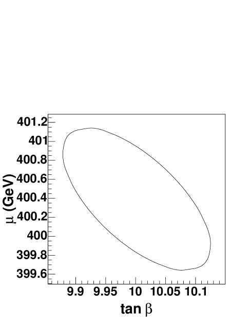
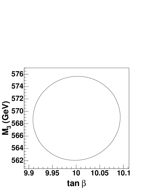
Figure 4: Examples of the two-dimensional uncertainty contours of the Fittino SPS1a’ fit.

A.4 Examples for the Pull Distributions

If parameter values and uncertainties (as determined with Fittino) are supplied for each parameter specified with fitParameter, pull distributions and the $\chi^{2}$ distribution of the fit is automatically calculated by Fittino if the flag CalcPullDist is set. Examples for these distributions, as obtained in a fit in the SPS1a scenario with 20 parameters, can be found in Figures 5 and 6.

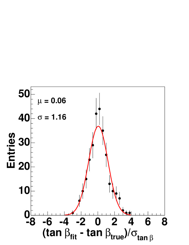
Figure 5: Pull distributions of the parameter $\tan\beta$ of the SPS1a’ fit for 120 independent fits with observables smeared within their uncertainties. The uncertainties of all parameters are well described.

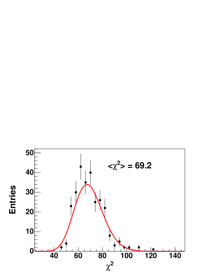
Figure 6: Distribution of $\chi^{2}$ for the SPS1a’ fit. 273 fits with 71 d.o.f. are performed. The observables of the simulated measurements are smeared in each fit according to their uncertainties. The mean of the distribution is $\chi^{2}_{\mathrm{mean}}=69.2$, in agreement with the expectation of $71\pm 0.9$.

A.5 Examples for the Observable Importance Determination

In the observable importance determination (using CalcIndChisqContr), the individual contribution of each observable to the determination of each parameter is calculated. Additionally, the total $\Delta\chi^{2}$ with respect to the minimal $\chi^{2}$ for a variation of $\pm 1\sigma$ of each parameter is shown. If the total $\Delta\chi^{2}$ is large, then the parameter is strongly correlated with other parameters. If it is close to 1, then there is hardly any correlation. In the output file fittino_individual_chisq_contr.out, for each parameter first all individual $\Delta\chi^{2}$ values from each observable are shown, followed by the percentage of the contribution from the 5 largest contributors. For the cross sections, the alias number is also shown in order to ensure the identification of cross sections at different polarisations and centre-of-mass energies.

Individual Delta Chisq contributions to Parameter TanBeta (10.0005 +- 0.333429)
================================================================

        list of all observables     :          Delta chi^2
                      .
                      .

                massNeutralino1     :             0.843007
                massNeutralino2     :              2.70032
                  massChargino1     :            0.0617443
                  massChargino2     :          0.000608651
ee  -> Neutralino1 Neutralino2 (19) :            0.0101081
ee  -> Neutralino2 Neutralino2 (20) :            0.0636789
 ee  -> SelectronL SelectronL~ (23) :           0.00277659
             ee  -> SmuL SmuL~ (25) :          0.000133514
           ee  -> Stau1 Stau1~ (27) :          0.000536534
           ee  -> Stau1 Stau1~ (28) :           0.00530975
    ee  -> Chargino1 Chargino1 (41) :            0.0489321
                   ee  -> Z h0 (45) :           0.00190326
                   ee  -> Z h0 (46) :            0.0012801
                      .
                      .

=========== percentage of strongest contributions: =============
                massNeutralino2     :             0.280837
ee  -> Neutralino2 Neutralino2 (20) :             0.191446
    ee  -> Chargino1 Chargino1 (41) :             0.126957
                massNeutralino1     :            0.0876738
ee  -> Neutralino1 Neutralino2 (19) :            0.0717215
              total Delta Chisq     :      9.615270


Individual Delta Chisq contributions to Parameter Mu (358.644 +- 1.14432)
================================================================
                      .
                      .

References

- [1] P. Bechtle, K. Desch, and P. Wienemann http://www-flc.desy.de/fittino.
- [2] SPA working group http://spa.desy.de/spa.
- [3] SPA working group draft available at http://spa.desy.de/spa.
- [4] T. Plehn (2004), hep-ph/0410063.
- [5] R. Lafaye, T. Plehn, and D. Zerwas http://sfitter.web.cern.ch/SFITTER/.
- [6] P. Skands et al. (2003), hep-ph/0311123.
- [7] W. Porod, Comput. Phys. Commun. 153(2003) 275, hep-ph/0301101.
- [8] P. Bechtle, K. Desch, and P. Wienemann Determination of MSSM Parameters from LHC and ILC Observables in a Global Fit, to appear.
- [9] H. U. Martyn (1999), hep-ph/0002290.
- [10] A. Corona et al., ACM Transactions on Mathematical Software 13(1987) 262.
- [11] W. L. Goffe, G. D. Ferrier, and J. Rogers, Journal of Econometrics 60(1994) 65.
- [12] F. James and M. Roos, Comput. Phys. Commun. 10(1975) 343.
- [13] P. M. Zerwas et al. (2002), hep-ph/0211076.
- [14] K. Desch, J. Kalinowski, G. Moortgat-Pick, M. M. Nojiri, and G. Polesello, JHEP 02(2004) 035, hep-ph/0312069.
- [15] W. Porod (1998), PhD thesis U. Vienna, hep-ph/9804208.
- [16] B. C. Allanach et al., Eur. Phys. J. C25(2002) 113, hep-ph/0202233.
- [17] G. Weiglein et al. [LHC/LC Study Group], “Physics interplay of the LHC and the ILC,” arXiv:hep-ph/0410364, Submitted to Phys.Rept.
- [18] R. Brun and F. Rademakers, Nucl. Instrum. Meth. A389(1997) 81.