MILOU : a Monte-Carlo for Deeply Virtual Compton Scattering

E. Perez^a, L. Schoeffel^a, L. Favart^b

^a CE Saclay, DAPNIA-SPP, 91191 Gif-sur-Yvette, France

^b ULB, Boulevard du Triomphe, 1050 Bruxelles, Belgium

Abstract

In this note, we present a new generator for Deeply Virtual Compton Scattering processes. This generator is based on formalism of Generalized Partons Distributions evolved at Next Leading Order (NLO). In the following we give a brief description of this formalism and we explain the main features of the generator for the elastic reactions, as well as for proton dissociation.

1 Introduction

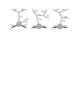
Figure 1: The contributing diagrams for the reaction $ep\rightarrow e\gamma p$ : (a) diagram for the Deeply Virtual Compton Scattering process ; (b) and (c) diagrams for Bethe-Heitler process.

Deeply Virtual Compton Scattering (DVCS) is the exclusive production of a real photon in diffractive $lepton-hadron$ interactions, $l+N\rightarrow l+\gamma+N$, as shown in Fig. 1 (a). This process is calculable in perturbative QCD (pQCD), when the virtuality, $Q^{2}=-q^{2}$, of the exchanged photon is large and it interferes with the purely electro-magnetic Bethe-Heitler (BH) reaction presenting the same final state (Fig. 1 (b) and (c)).

The first measurements of the DVCS process at high $W^{2}=(q+P)^{2}$ [1, 2] and its beam-spin asymetry in polarised $ep$ scattering at low $W^{2}$ [3, 4] have recently become available. A proposal for dedicated studies at the COMPASS experiment (in $\mu p$ collisions) is also under review.

The DVCS reaction can be regarded as the elastic scattering of the virtual photon off the proton via a colourless exchange. The pQCD calculations assume that the exchange involves two partons, having different longitudinal and transverse momenta, in a colourless configuration. These unequal momenta are a consequence of the mass difference between the incoming virtual photon and the outgoing real photon. The DVCS cross section depends, therefore, on the Generalised Parton Distributions (GPD), which carry information about parton correlations inside a nucleon.

First predictions for DVCS cross sections were based on LO calculations [5]. These calculations explicitely involve the variable R defined as the ratio of the imaginary part for the amplitudes for DIS and DVCS processes :

$$R=\frac{Im(A(\gamma^{*}p\rightarrow\gamma^{*}p))}{Im(A(\gamma^{*}p\rightarrow\gamma p))}$$

A value of $R\simeq 0.55$ has been shown to be in good agreement with HERA results. Previous Monte-Carlo (MC) for DVCS generation are based on this approach [6, 7]. We refer to this prediction as FFS (Frankfurt-Freund-Strikman) in the following [5].

However, even if this effective LO prediction reproduces correctly the experimental data, it is not sufficient as it does not provide a direct insight of the rich information present in GPDs. The MC described in this note has been developped to allow experimental measurements to be compared with GPD models and to study asymetries.

GPDs have been studied extensively in recent years [8, 9, 10]. These distributions are not only the basic, non-perturbative ingredient in hard exclusive processes such as DVCS or exclusive vector meson production, but they are also generalizations of the well known Parton Distribution Functions (PDFs) from inclusive reactions.

In the approach developped in reference [8], the scattering amplitude is simply given by the convolution of a hard scattering coefficient computable to all orders in perturbation theory with one type of GPD carrying the non-perturbative information. The formalism for the NLO QCD evolution equations for GPDs can be found in reference [11].

Higher twists contributions to the DVCS amplitude have been calculated in reference [8]. They consist in terms of order $O(m_{N}/Q)$, $O(\sqrt{-t}/Q)$ and $O(\lambda_{QCD}/Q)$ with $m_{N}$ the proton mass and $t=(P-P^{\prime})^{2}$ the momentum transfer to the outgoing proton. They have been shown to be sizeable at low $Q^{2}$ within the kinematic domain relevant for HERMES, CLAS or COMPASS experiments.

2 Structure of the MC program

The core of the program consits of several fortran routines provided by A. Freund. The calculations of cross sections from GPDs are done in two steps :

• The GPDs $H,{\tilde{H}},E,{\tilde{E}}$ are evolved at NLO by an independent code [12] which provides tables for the real and imaginary parts of the so called Compton Form Factor (CFFs) : at LO, they are just the convolution of GPDs by the coefficient functions [8]. For example

  $${\cal H}(\xi,Q^{2},t)={\displaystyle\sum_{u,d,s}}\int_{-1}^{1}[\frac{e_{i}^{2}}{1-x/\xi-i\epsilon}\pm\{\xi\rightarrow-\xi\}]H_{i}(x,\xi,Q^{2},t)dx$$

  with $e_{i}$ the fractional quark charge and $\xi=x_{B}/(2-x_{B})$ the skewing variable. There are different tables for each GPD and for LO/NLO approximations, as well as for the twists-3 corrections. The GPDs parameterisations at the initial scale (in $Q^{2}$) are described in reference [8].

  In the DGLAP domain, they consist in distributions based on the forward CTEQ6 parameterisations [13], with no external skeewing added in a profile function. In each table, there are 48 bins in $x_{B}=\frac{Q^{2}}{2Pq}$ extending from $10^{-4}$ till $0.7$ and for each of them 40 bins in $Q^{2}$ from $1$ GeV² till $10^{4}$ GeV² (regularly spaced in $\ln Q^{2}$). We obtain the values for the real and imaginary parts of the CFFs considered after a 2D spline of the $x_{B}-Q^{2}$ grid.

• From these CFFs, the cross sections for DVCS and BH-DVCS interference are calculated according to formulae of reference [8] (see section 3). The BH cross section is also calculated according to standard expressions. During the iterative integration step, the code provides an output with the estimated cross-section and the accuracy of the integration. It is always important to check the proper convergence of the integrals and that the final accuracy is small (below $1\%$), which means that no problem have occured in the integration over the kinematic range considered.

The squared amplitudes are first integrated within the kinematic domain defined by the user. Events are then generated according to the differential cross sections. These two steps make use of the BASES/SPRING package [14]. For each accepted event, the kinematics of the final state particles is stored into a PAW ntuple. The relevant kinematic formuae are detailed in section 3.2. The generated events are stored in the standard LUJETS common of the PYTHIA [15] program.

3 Cross section formulae and kinematics

In the MC, we are calculating the five-fold cross section for the DVCS process

$$\frac{d\sigma}{dx_{\rm B}dyd|t|d\phi d\varphi}=\frac{\alpha^{3}x_{\rm B}y}{16\,\pi^{2}\,{Q}^{2}\sqrt{1+\epsilon^{2}}}\left|\frac{\cal T}{e^{3}}\right|^{2}$$ (1)

in which the amplitude ${\cal T}$ is the sum of the DVCS and Bethe-Heitler (BH) amplitudes : ${\cal T}={\cal T}_{\rm DVCS}+{\cal T}_{\rm BH}$. This cross section depends on the Bjorken variable $x_{\rm B}$, the squared momentum transfer $t=(P-P^{\prime})^{2}$, the lepton energy fraction $y=P\cdot q/P\cdot k$, and, in general, two azimuthal angles. We use the convention $\epsilon\equiv 2x_{\rm B}\frac{m_{N}}{{Q}}$.

In equation (1), $\phi=\phi_{N}-\phi_{l}$ is the angle between the lepton and hadron scattering planes and $\varphi={\mit\Phi}-\phi_{N}$ is the difference of the azimuthal angle $\mit\Phi$ of the transverse part of the nucleon polarisation vector $S$, i.e., $S_{\perp}=(0,\cos{\mit\Phi},\sin{\mit\Phi},0)$, and the azimuthal angle $\phi_{N}$ of the recoiled hadron. Our frame is rotated with respect to the laboratory one in such a way that the virtual photon four-momentum has no transverse components, see Fig. 2. For the kinematics we choose the following convention : the $z$-component of the virtual photon momentum is negative and $x$-component of the incoming lepton is positive with $k=(E,E\sin\theta_{l},0,E\cos\theta_{l})$, $q=(q_{0},0,0,-|q_{3}|)$. Other vectors are $P=(M,0,0,0)$ and $P^{\prime}=(E_{2},|\mbox{\boldmath$P$}_{2}|\cos\phi\sin\theta_{N},|\mbox{\boldmath$P$}_{2}|\sin\phi\sin\theta_{N},|\mbox{\boldmath$P$}_{2}|\cos\theta_{N})$.

Figure 2: The kinematics of the leptoproduction in the target rest frame. In this figure taken from reference [8], $k$, $k^{\prime}$, $P_{2}$ and $q_{2}$ are respectively the four-momenta of the initial lepton, the scattered lepton, the outgoing proton and the real photon. The $z$-direction is chosen counter-along the three-momentum of the incoming virtual photon. The lepton three-momenta form the lepton scattering plane, while the recoiled proton and outgoing real photon define the hadron scattering plane. In this reference system the azimuthal angle of the scattered lepton is $\phi_{l}=0$, while the azimuthal angle between the lepton plane and the recoiled proton momentum is $\phi_{N}=\phi$. When the hadron is transversely polarised (in this reference frame) $S_{\perp}=(0,\cos{\mit\Phi},\sin{\mit\Phi},0)$, the angle between the polarisation vector and the scattered hadron is denoted as $\varphi={\mit\Phi}-\phi_{N}$.

3.1 Cross sections

The BH amplitude is real (to the lowest order in the QED fine structure constant) and is parameterised in terms of electromagnetic form factors, which we assume to be known from other measurements.

According to reference [8], the BH, DVCS and interference terms of equation (1), namely $|{\cal T}_{\rm BH}|^{2}$, $|{\cal T}_{\rm DVCS}|^{2}$ and ${\cal I}={\cal T}_{\rm DVCS}{\cal T}_{\rm BH}^{*}+{\cal T}_{\rm DVCS}^{*}{\cal T}_{\rm BH}$ can be written :

$$|{\cal T}_{\rm BH}|^{2}=\frac{e^{6}}{x_{\rm B}^{2}y^{2}(1+\epsilon^{2})^{2}\Delta^{2}\,{\cal P}_{1}(\phi){\cal P}_{2}(\phi)}\left\{c^{\rm BH}_{0}+\sum_{n=1}^{2}c^{\rm BH}_{n}\,\cos{(n\phi)}+s^{\rm BH}_{1}\,\sin{(\phi)}\right\}$$ (2)

$$|{\cal T}_{\rm DVCS}|^{2}=\frac{e^{6}}{y^{2}{\cal Q}^{2}}\left\{c^{\rm DVCS}_{0}+\sum_{n=1}^{2}\left[c^{\rm DVCS}_{n}\cos(n\phi)+s^{\rm DVCS}_{n}\sin(n\phi)\right]\right\}$$ (3)

$${\cal I}=\frac{\pm e^{6}}{x_{\rm B}y^{3}\Delta^{2}{\cal P}_{1}(\phi){\cal P}_{2}(\phi)}\left\{c_{0}^{\cal I}+\sum_{n=1}^{3}\left[c_{n}^{\cal I}\cos(n\phi)+s_{n}^{\cal I}\sin(n\phi)\right]\right\}$$ (4)

where the $+$ ($-$) sign in the interference stands for the negatively (positively) charged lepton beam. In this expression, the Fourier coefficients $c_{i}$, $s_{i}$ are fonction of CFFs (and then GPDs) and $1/{\cal P}_{1}$ and $1/{\cal P}_{2}$ are the lepton BH propagators.

We have mentioned above that the real and imaginary parts of the CFFs (convolution of the GPDs by a hard coefficient function) are given in tables of $x_{B}-Q^{2}$, thus the $t$ dependence is assumed to be factorised and has to be defined by the MC user. We have included an option in the steering which allows to consider a global exponential behaviour of the cross section

$$d\sigma/dt\propto exp(B(Q^{2})\ t)$$

in which the $t$ slope $B(Q^{2})$ can be chosen as a linear function of $\ln Q^{2}$. Alternatively, the $t$ dependence can also be given by the Pauli-Dirac form factors for each GPD flavor.

3.2 Event kinematics

The reconstruction of energies and angles of the scattered positron, photon and proton is carried out for each event from $x$, $Q^{2}$, $t$ and $\phi$.

The kinematics of the outgoing lepton (and then of the virtual photon) is trivially obtained in the laboratory frame. The kinematics of the outgoing nucleon

$$P^{\prime}=(E_{2},|\mbox{\boldmath$P$}_{2}|\cos\phi\sin\theta_{N},|\mbox{\boldmath$P$}_{2}|\sin\phi\sin\theta_{N},|\mbox{\boldmath$P$}_{2}|\cos\theta_{N})$$

is most easilly obtained in the the frame of Fig. 1, where the target nucleon is at rest. We use

$$E_{2}=m_{N}-\frac{t}{2m_{N}}\ \ \ \ \ |\mbox{\boldmath$P$}_{2}|=\frac{\sqrt{t(t-4m_{N}^{2})}}{2m_{N}}$$

and

$$\cos\theta_{N}=\frac{(q_{3})^{2}-(q_{0})^{2}+|\mbox{\boldmath$P$}_{2}|^{2}}{2|\mbox{\boldmath$P$}_{2}|\ q_{3}}$$

in which the virtual photon components can be expressed as

$$q_{0}=\frac{t+Q^{2}/x_{B}}{2m_{N}}\ \ \ \ \ q_{3}=-\frac{Q^{2}}{2m_{N}x_{B}}\sqrt{1+\frac{4m_{N}^{2}x_{B}^{2}}{Q^{2}}}$$

After a Lorentz transformation, we finally get all variables (energies and angles of incoming and outgoing particles) in the laboratory frame. In the ntuple produced during the generation, these variables are given in both frames.

4 Integration and Generation

Integration and generation are realized with the BASES/SPRING package [14]. By BASES, probability distributions are calculated by integrating the differential cross-section over the phase space and saved in a file which is then used in the generation step. By SPRING, events are generated by the MC method according to the above distributions.

5 Proton dissociation

It has been shown that the proton dissociation is a non negligible contribution (10% to 20%) in the measured DVCS samples for H1 and ZEUS experiments [1, 2]. Thus, it is important to include this process in the MC.

In case of proton dissociation the DVCS process $ep\rightarrow eY\gamma$ leads to a state of mass $M_{Y}$ and the generation of the $M_{Y}$ spectrum follows the parameterisation exposed in [16], as it is done in the DIFFVM MC [17]. The main hypothesis is that $\frac{d\sigma}{dM_{Y}^{2}}$ can be factorised with the elastic DVCS cross-section, with :

$$\frac{d\sigma}{dM_{Y}^{2}}=\frac{f(M_{Y}^{2})}{M^{2(1+\epsilon)}}$$

In the continuum region ($M_{Y}^{2}>3.6$ GeV²), $f(M_{Y}^{2})=1$ leading to a global $M_{Y}$ dependence in $1/M^{2(1+\epsilon)}$ for proton dissociation. In the resonance region ($M_{Y}^{2}<3.6$ GeV²), $f(M_{Y}^{2})$ is the result of a fit for the proton diffractive dissociation on deuterium (at fixed $t$) [16]. It is important to note that this treatment is only acceptable for DVCS at large $W$ ($W>20$ GeV). Thus, it must not be applied in the BH mode and in the low $W$ domain, where the stucture of resonances is more complex.

6 Examples

6.1 Elastic DVCS process

To illustrate the ouput of the DVCS MC, we first present some examples in the elastic case ($ep\rightarrow ep\gamma$). In Fig. 3 we present the generated kinematic variables in the range $10^{-4}\leq x_{Bj}\leq 0.1$, $4\leq Q^{2}\leq 100$ GeV² and $t>-1$ GeV². The generation is done at NLO for different $t$ dependences of the GPDs as explained in the caption of Fig. 3. For the same generation, Fig. 4 represents the spectra for energies and polar angles of the outgoing particles. The normalization is done to the number of events.

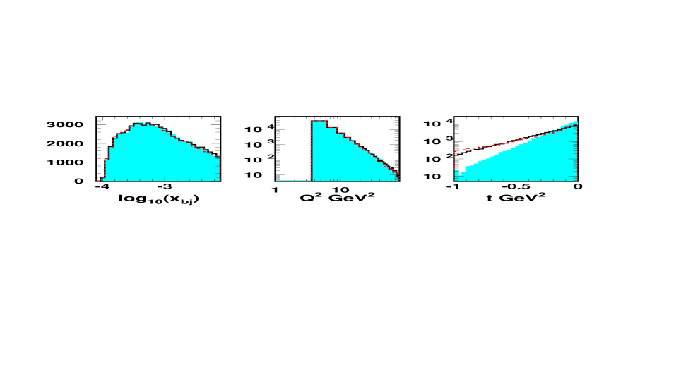
Figure 3: Predictions for the kinematic variables at NLO of the DVCS MC for different behaviours in $t$ : the full histogram stands for a global exponential $t$ dependence of the DVCS cross section in $e^{B\ t}$ with $B=7$ GeV^-2 ; the full line represents also an exponential $t$ dependence with a slope of $B=4$ GeV^-2 and the dotted line has been obtained when considering the Dirac-Pauli form factors for each GPDs. Histograms are normalized to the number of events.

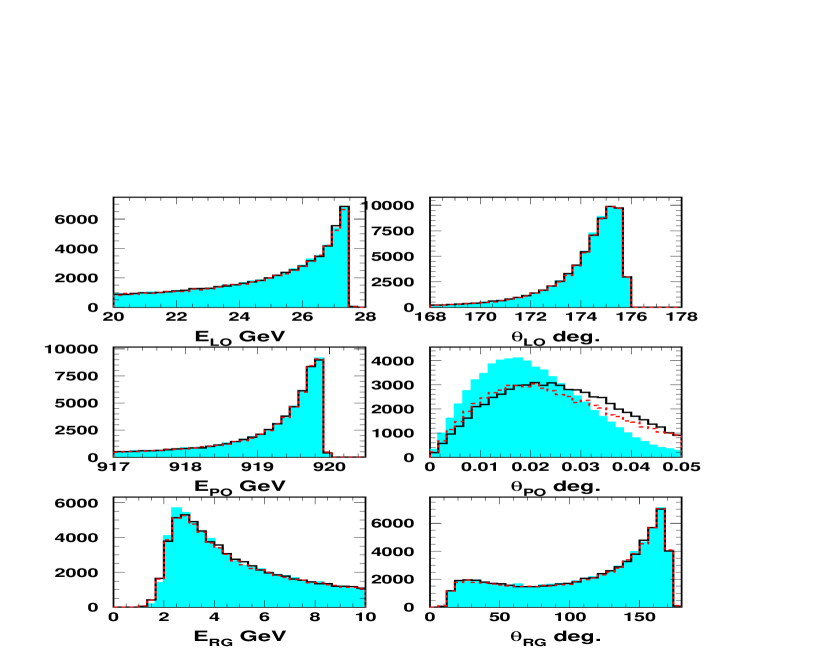
Figure 4: With the same convention as in Fig. 3, (different t dependences), we represent the energies and angles of the scattered (outgoing) lepton $E_{LO}$ and $\theta_{LO}$, for the outgoing proton $E_{PO}$ and $\theta_{PO}$ and for the real photon $E_{RG}$ and $\theta_{RG}$.

In Fig. 5, we show the coplanarity (absolute difference of the azimuthal angles of the scattered lepton and real photon) of the elastic DVCS process (again with the three different $t$ behaviours considered since Fig. 3). We observe the broadening of this distribution when the $t$ slope becomes larger. Indeed, for small momentum transfer the $e\gamma$ system is balanced and the coplanarity is close to $180^{o}$, whereas for larger momentum transfer the $e\gamma$ system becomes unbalanced and a deviation form $180^{o}$ is observed. And, of course, the fraction of events with a large momentum transfer is enhanced when $B$ becomes smaller.

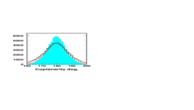
Figure 5: Coplanarity : absolute difference of the azimuthal angles of the scattered lepton and real photon, for the three cases mentioned in Fig. 3.

As mentioned in section 1, previous measurements (and then acceptance corrections) at low $x_{B}$ [1, 2] are based on the FFS approximation for the DVCS cross-section [5]. On Fig. 6, we compare the FFS (for R=0.55) and NLO predictions of the DVCS MC in the same generated kinematic range : $10^{-4}\leq x_{Bj}\leq 0.1$, $4\leq Q^{2}\leq 100$ GeV² and $t>-1$ GeV². For this comparison we only consider a global exponential $t$ dependence with $B=7$ GeV^-2. Histograms are normalized to the number of events and we notice a good agreement in shapes. However the cross section calculated in the NLO case is calculated to be about $15\%$ higher than the LO FFS one (for the GPDs parameterisations included in the code). Regarding the good agreement in shapes, one can wonder whether it is useful to extend the MC from FFS LO to NLO GPDs calculations. However, it is important to note at this stage that GPDs at NLO become essential to predict asymetries as explained later in this note. Also, as mentioned previously, with GPDs we can consider different $t$ dependences for the different flavors, which is obviously not possible in the FFS approximation.

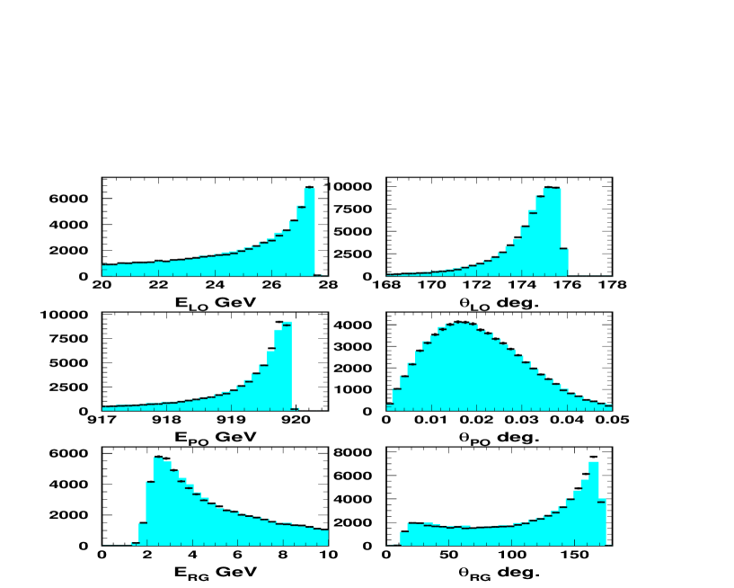
Figure 6: Comparisons of the predictions based on the LO calculations [5] with a value of $R=0.55$ (black points) and of the NLO calculations (full histogram). In both cases, we have considered a global exponential $t$ dependence with $B=7$ GeV^-2. Histograms are normalized to the number of events.

6.2 DVCS vs BH cross-sections

In Fig. 7 we present another illustration of the MC : we compare the DVCS with the BH process when the lepton is scattered backward ($\theta_{lo}>160^{o}$), the real photon is scattered with $\theta_{rg}<160^{o}$ and the azimuthal angle is integrated over. This configuration is the one analysed in H1 and ZEUS experiments to extract the DVCS cross-sections [1, 2]. Histograms (Fig. 7) are normalized to luminosities and the interference between DVCS and BH is calculated to be negligible : as the azimuthal angle is integrated over, the constant term in the expression for the interference (see formula 4) is the only (negligible) contribution. We notice the different behaviours in $W$, $E_{lo}$, which allow a good separation power at low $W$ ($W\leq 120$ GeV) and large $E_{lo}$ ($E_{lo}\geq 15$ GeV) and thus allow the measurement of the DVCS cross-section.

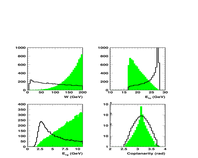
Figure 7: Spectra of DVCS (full line) compared to BH (full histogram) processes for $W$, energies of the outgoing lepton and the real photon and the coplanarity. The configuration considered for these plots is the one with the lepton scattered backward ($\theta_{lo}>160^{o}$) and the real photon scattered with $\theta_{rg}<160^{o}$. Histograms are normalized to luminosities as calculated by the MC.

In Fig. 8 we compare DVCS and BH when both lepton and photon are scattered backward ($\theta_{lo,rg}>160^{o}$). Histograms are normalized to luminosities. We notice that in this case the BH process is dominating, the DVCS representing about $6\%$ of the sample and the interference about $0.5\%$.

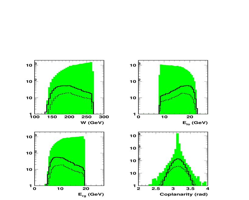
Figure 8: Spectra for DVCS (full line) compared to BH (full histogram) processes for $W$, energies of the outgoing lepton and the real photon and the coplanarity. The configuration considered for these plots is the one with the lepton and the real photon scattered backward ($\theta_{lo,rg}>160^{o}$). Histograms are normalized to luminosities as calculated by the MC. In this configuration, it is interesting to notice that the interference (dotted line) is small but non negligible (about $0.5\%$) of the BH sample.

6.3 Proton dissociation DVCS process

As mentioned in section 5, in case of proton dissociation the DVCS process $ep\rightarrow eY\gamma$ leads to a state of mass $M_{Y}$. We present on Fig. 9 the generated $M_{Y}$ for two values of the $t$ slope (slope of the global exponential $t$ dependence). As mentioned in section 5, we notice the $M_{Y}$ behaviour in

$$\frac{d\sigma}{dM_{Y}^{2}}=\frac{f(M_{Y}^{2})}{M^{2(1+\epsilon)}}$$

with the resonance region at low $M_{Y}$ ($M_{Y}^{2}<3.6$ GeV²) and the $1/M^{2(1+\epsilon)}$ shape at larger values.

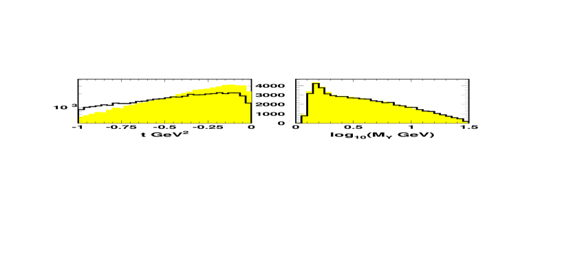
Figure 9: Example of predictions of the DVCS MC for proton dissociation. With two values of $B$ (slope of the global exponential $t$ dependence) : $B=1$ GeV^-2 (black line) and $B=2$ GeV^-2 (full histogram), we represent the $t$ spectrum and the generated mass of the proton dissociated system $M_{Y}$ (in log).

Away from the resonance region, the system $Y$ is treated as a quark-diquark (q-qq) system. Its hadronisation is performed by PYTHIA. We have added an option compared to the treatment done in the DIFFVM MC. In DIFFVM, it is assumed that the proton splits into a q-qq system, so that the quark couples to the pomeron leaving a diquark remnant. Due the possible spin states of this diquark system (in a singlet or triplet wave function), different probabilities are assigned to the different configurations of the q-qq system. However, for a DVCS process, the coupling of the valence quark can also be done to a quark : see for example the LO handbag diagram. Thus, the probabilities for the q-qq system describing the proton have to be modified by taking into the account the electric charge coupling. We have introduced a real parameter in the steering which allows to define the type of probabilities considered : $\alpha=0$ if we only consider the probabilities defined by spin states $P_{0}$ , $\alpha=1$ in case of spin states and electric coupling ${P_{1}}$, and $0<\alpha<1$ for ${P_{\alpha}=(1-\alpha)P_{0}+\alpha P_{1}}$.

7 Steering cards

EXP 1 : 1/0 to use de logarithmic/linear binning in the kinematic range for $Q^{2}$ and $x_{B}$

SEED 2345671 : generation seed value

FIXED FALSE : FALSE/TRUE to select collider/fixed-target modes

ELEP -27.55 : beam momentum (in GeV/c) of the lepton beam

ETARG 920. : in collider mode, beam momentum (in GeV/c) of the proton beam or, in fixed target mode, mass of the target

LCHAR +1. : lepton charge in units of $e$ in case TINTIN is set to FALSE (the code is using the grids of real and imaginary parts for CFFs)

LPOL 0. : polarisation of lepton, +1 in direction of movement, -1 against direction of movement, 0 for unpolarised

TPOL 0. : target polarisation, +1(-1) = polarised along (opposite) probe/target beam direction, 0 for unpolarised

ZTAR 1. : charge of the target

ATAR 1. : atomic number of the target

SPIN 1. : spin of target nucleon type (in units of ${\hbar}/2$)

IRAD 0 : 1 for QED radiative corrections to be applied, 0 otherwise (only the ISR are included in the code)

IELAS 1 : 1 to run the code for the elastic case only, 0 to run in the proton dissociation mode only. Note that we can not run both cases together and, as mentioned above, the proton dissociation treatment implemented in the code can only be used for a pure DVCS process

IRFRA 1 : in case of proton dissociation for the resonances domain, IRFRA=0 if the user wants to use DIFFVM’s routines for the decays of resonances, 1 if this user wants to decay via PYTHIA

PROSPLIT 1. : treatment of dissociated proton in the continuum domain, PROSPLIT $\equiv\alpha$ (see above) steers how the proton is splitted into quark-diquark

EPSM 0.08 : for proton dissocation, EPSM $\equiv\epsilon$ with $d\sigma/dM_{Y}^{2}\propto 1/M_{Y}^{2(1+\epsilon)}$

TINTIN FALSE : TRUE to run in the LO FFS [5] approximation, FALSE to use the grids for CFFs

BTIN 2. : slope of the exponential t dependence (in the FFS approximation)

RTIN 0.55 : value for the variable $R=\frac{Im(A(\gamma^{*}p\rightarrow\gamma^{*}p))}{Im(A(\gamma^{*}p\rightarrow\gamma p))}$ (see section 1)

F2QCD TRUE : in the FFS approximation $\sigma_{DVCS}\propto F_{2}^{2}/R^{2}$, this parameter determines the parameterisation considered for $F_{2}$ : TRUE/FALSE respectively for the H1 QCD fit or ALLM results

DIPOLE FALSE : if the parameter TINTIN is TRUE, it’s possible to run the code using the diople model formula (in this case DIPOLE must be set to TRUE)

IGEN 0 : generation mode with BASES/SPRING : 0 for the grid calculation and the generation and 4 for the generation only (which requires the file bases.data)

NGEN 10 : dummy

NPRINT 10 : number of events for which the PHYTHIA output is printed

NCALL 10000 : parameter for BASES, number of sampling points per iteration

ITMX1 10 : parameter for BASES, number of iterations for the grid defining step

ITMX2 10 : parameter for BASES, number of iterations for the integration step

IDEBUG 0 : debug flag

NXGRID 58 : Number of $X$ points in the CFFs grids

NQGRID 40 : Number of $Q^{2}$ points in the CFFs grids

IPRO 2 : process to generate : 1,2,3,4 or 5 for BH, DVCS, interference BH-DVCS, charge asymetry or single spin asymetry respectively.

IORD 2 : order for the calculations of the GPDs amplitudes : 1/2 for LO/NLO

XMIN 1.0e-4 : lower bound of $x_{B}$ for the kinematic domain of the generation. If the MC user run the code with the use of CFFs grids, this value must be larger than the lower bound of the grids ($10^{-4}$ in our case)

XMAX 1.0e-1 : upper bound of $x_{B}$

QMIN 3.0 : lower bound for $Q^{2}$ (in GeV²)

QMAX 300.0 : upper bound for $Q^{2}$ (in GeV²)

TMIN 0.0 : upper bound for $t=(p^{\prime}-p)^{2}$ (in GeV²)

TMAX -1.5 : lower bound for $t=(p^{\prime}-p)^{2}$ (in GeV²)

MYMIN 1.13 : lower bound on $M_{Y}$ in proton dissociation case

MYMAX 30. : upper bound on $M_{Y}$

NSET 2 : integration over PHI $\equiv\phi$ : 2 for integration, 1 otherwise

PHI 0. : in case of NSET=1, azimuthal angle between lepton and final state scattering planes

PPHI 0. : in case of NSET=1, angle between lepton plane and transverse polarisation vector

THETA 0. : angle between longitudinal and transverse polarisation

TWIST3 FALSE : Twists 3 calculations (TRUE) or not (FALSE)

ITFORM 0 : in case of the use of CFFs grids, if ITFORM=0, the $t$ dependence is in $\exp(bt)$ with $b=$ BQCST $+$ BQSLOPE $\log(Q^{2}/Q0SQ)$ ; if ITFORM=2, the Pauli-Dirac form factors are used for the $t$ dependence ; finally, if ITFORM=4, the $t$ dependence is in $\exp(bt)$ for $x_{B}<$ X0DEF and Pauli-Dirac form factors are considered otherwise. Note that in case of the LO FFS approximation the $t$ dependence is set by the parameter BTIN (see above).

BQCST 7.0 : see ITFORM

BQSLOPE 0.0 : see ITFORM

BGCST 7.0 : see ITFORM

BGSLOPE 0.0 : see ITFORM

Q0SQ 2.0 : see ITFORM

X0DEF 0.1e0 : see ITFORM

THLMIN 00.0 : lower bound on $\theta_{lepton}$ (in deg.)

THLMAX 180.0 : upper bound on $\theta_{lepton}$ (in deg.)

ELMIN 10.0 : lower value of $E_{vis}$ (in GeV)

THGMIN 00.0 : lower bound on $\theta_{\gamma}$ (in deg.)

THGMAX 180.0 : upper bound on $\theta_{\gamma}$ (in deg.)

EIMIN 0.00001 : minimum value for the ISR photon (in GeV)

YMAX 0.4 : maximum value for $y=Q^{2}/(sx)$

M12MIN 1. : minimum value for the reconstructed mass of the outgoing lepton and the real photon

ELMB 0. : minimum value of the outgoing lepton energy (in GeV)

EGMB 0. : minimum value of the real photon energy (in GeV)

8 Summary

MILOU is a new generator for DVCS based on the formalism of Generalized Partons distributions. This MC has been developped to allow experimental measurements to be compared with GPD models (at LO or NLO) and to study asymetries. The generation of BH processes and interference between DVCS and BH are also aviable. In addition, in case of pure DVCS we have included the possiblility to study proton dissociation.

9 Acknowledgements

We are very thankfull to A. Freund and M. McDermott for providing us tables with Compton Form Factors and the core of code for DVCS cross-section calculations. We also wish to thank A. Bruni for helpful discussion on proton dissociation.

References

- [1] H1 collab., C. Adloff et al., Phys. Lett. B 517, 47 (2001).
- [2] ZEUS collab., S. Chekanov et al., Phys. Lett. B 578, 33 (2004).
- [3] HERMES collab., A. Airapetian et al., Phys. Rev. Lett. 97, 182001 (2001).
- [4] CLAS collab., S. Stepanyan et al., Phys. Rev. Lett. 87 182002 (2001).
- [5] L. Frankfurt, A. Freund, M. Strikman, Phys. Lett. B 460, 417 (1999).
- [6] R. Stamen, PhD dissertation, Universität Dortmund and Univ. Libre de Bruxelles, in preparation, made available through: http://www-h1.desy.de/publications/theses_list.html
- [7] P.R.B. Saull, GenDVCS, http://www-zeus.desy.de/physics/diff/pub/MC
- [8] A.V. Belitsky, D. Muller and A. Kirchner, Nucl. Phys. B 629, 323 (2002) ; A. Freund, Phys.Rev. D 68 096006 (2003).
- [9] A. Freund and M. McDermott, Phys. Rev. D 65, 091901 (2002).
- [10] M. Diehl, Phys.Rept. 388 41-277 (2003), DESY-THESIS-2003-018, hep-ph/0307382.
- [11] A.V. Belitsky, A. Freund and D. Muller, Nucl. Phys. B 574, 347 (2000) ; Phys. Lett. B 493, 341 (2000).
- [12] A. Freund, private communication.
- [13] J. Pumplin, D.R. Stump, J.Huston, H.L. Lai, P. Nadolsky, W.K. Tung, JHEP 0207:012 (2002).
- [14] S. Kawabata, Comp. Phys. Comm. 41 127 (1986).
- [15] T. Sj strand, P. Ed n, C. Friberg, L. L nnblad, G. Miu, S. Mrenna and E. Norrbin, Computer Phys. Commun. 135 (2001) 238.
- [16] K. Goullianos, Phys. Rep. 101, No. 3, 169 (1983).
- [17] B. List, A. Mastroberardino, DIFFVM: A Monte Carlo generator for diffractive processes in ep scattering, Proceedings of the Monte Carlo Generators for HERA physics, DESY-PROC-1999-02, p. 396.