CERN-PH-TH/2004-237

TUM-HEP-569/04

MPP-2004-154

hep-ph/0411373

$B\to\pi\pi$, New Physics in $B\to\pi K$ and
Rare $K$ and $B$ Decays^†

Andrzej J. Buras,^a Robert Fleischer,^b Stefan Recksiegel^a and Felix Schwab^c,a

^a Physik Department, Technische Universität München, D-85748 Garching, Germany

^b Theory Division, Department of Physics, CERN, CH-1211 Geneva 23, Switzerland

^c Max-Planck-Institut für Physik – Werner-Heisenberg-Institut, D-80805 Munich, Germany

We summarize a recent strategy for a global analysis of the $B\to\pi\pi,\pi K$ systems and rare decays. We find that the present $B\to\pi\pi$ and $B\to\pi K$ data cannot be simultaneously described in the Standard Model. In a simple extension in which new physics enters dominantly through $Z^{0}$ penguins with a CP-violating phase, only certain $B\to\pi K$ modes are affected by new physics. The $B\to\pi\pi$ data can then be described entirely within the Standard Model but with values of hadronic parameters that reflect large non-factorizable contributions. Using the $SU(3)$ flavour symmetry and plausible dynamical assumptions, we can then use the $B\to\pi\pi$ decays to fix the hadronic part of the $B\to\pi K$ system and make predictions for various observables in the $B_{d}\to\pi^{\mp}K^{\pm}$ and $B^{\pm}\to\pi^{\pm}K$ decays that are practically unaffected by electroweak penguins. The data on the $B^{\pm}\to\pi^{0}K^{\pm}$ and $B_{d}\to\pi^{0}K$ modes allow us then to determine the electroweak penguin component which differs from the Standard Model one, in particular through a large additional CP-violating phase. The implications for rare $K$ and $B$ decays are spectacular. In particular, the rate for $K_{\rm L}\rightarrow\pi^{0}\nu\bar{\nu}$ is enhanced by one order of magnitude, the branching ratios for $B_{d,s}\to\mu^{+}\mu^{-}$ by a factor of five, and $\mathrm{BR}(K_{\rm L}\to\pi^{0}e^{+}e^{-},\pi^{0}\mu^{+}\mu^{-})$ by factors of three.

^† Talk presented by A. J. Buras at SUSY 04, June 17-23, 2004, Tsukuba, Japan
November 2004

Abstract

We summarize a recent strategy for a global analysis of the $B\to\pi\pi,\pi K$ systems and rare decays. We find that the present $B\to\pi\pi$ and $B\to\pi K$ data cannot be simultaneously described in the Standard Model. In a simple extension in which new physics enters dominantly through $Z^{0}$ penguins with a CP-violating phase, only certain $B\to\pi K$ modes are affected by new physics. The $B\to\pi\pi$ data can then be described entirely within the Standard Model but with values of hadronic parameters that reflect large non-factorizable contributions. Using the $SU(3)$ flavour symmetry and plausible dynamical assumptions, we can then use the $B\to\pi\pi$ decays to fix the hadronic part of the $B\to\pi K$ system and make predictions for various observables in the $B_{d}\to\pi^{\mp}K^{\pm}$ and $B^{\pm}\to\pi^{\pm}K$ decays that are practically unaffected by electroweak penguins. The data on the $B^{\pm}\to\pi^{0}K^{\pm}$ and $B_{d}\to\pi^{0}K$ modes allow us then to determine the electroweak penguin component which differs from the Standard Model one, in particular through a large additional CP-violating phase. The implications for rare $K$ and $B$ decays are spectacular. In particular, the rate for $K_{\rm L}\rightarrow\pi^{0}\nu\bar{\nu}$ is enhanced by one order of magnitude, the branching ratios for $B_{d,s}\to\mu^{+}\mu^{-}$ by a factor of five, and $\mathrm{BR}(K_{\rm L}\to\pi^{0}e^{+}e^{-},\pi^{0}\mu^{+}\mu^{-})$ by factors of three.

^a Physik Department, Technische Universität München, D-85748 Garching, Germany
^b Theory Division, Department of Physics, CERN, CH-1211 Geneva 23, Switzerland
^c Max-Planck-Institut für Physik – Werner-Heisenberg-Institut, D-80805 Munich, Germany

1 Introduction

The Standard Model (SM) for strong and electroweak interactions of quarks and leptons gives a very satisfactory description of the observed phenomena down to the short-distance scales of ${\cal O}(10^{-18})\,m$ or equivalently the scale of the top-quark mass. Exceptions are the non-vanishing neutrino masses, possibly related to scales of ${\cal O}(10^{-28})\,m$ through the see-saw mechanism, the observed matter–antimatter asymmetry of the Universe, possibly related to even lower scales, and the issue of the low Higgs mass, which is related to the so-called naturalness problem. One should, however, emphasize that, whereas the SM gauge sector of the electroweak interactions has been tested to a very high precision in the 1990s, studies of the flavour-changing interactions of quarks and leptons – in particular those involving CP-violating transitions – did not yet reach this precision and we should be prepared for surprises. Finally, the non-perturbative part of QCD has to be put under much better control.

In this context, the present studies of non-leptonic two-body $B$ decays and of rare $K$ and $B$ decays are very important as they will teach us both about the non-perturbative aspects of QCD and about the perturbative electroweak physics at very short distances. For the analysis of these modes, it is essential to have a strategy available that could clearly distinguish between non-perturbative QCD effects and short-distance electroweak effects. A strategy that in the case of deviations from the SM expectations would allow us transparently to identify a possible necessity for modifications in our understanding of hadronic effects and for a change of the SM model picture of electroweak flavour-changing interactions at short-distance scales.

In [?,?], we have developed a strategy that allows us to address these questions in a systematic manner. It encompasses non-leptonic $B$ and $K$ decays and rare $K$ and $B$ decays but has been at present used primarily for the analysis of $B\to\pi\pi$ and $B\to\pi K$ systems and rare $K$ and $B$ decays. The purpose of this note is to summarize the basic ingredients of our strategy and to list the most important results. A detailed update of the analyses in [?,?] has recently been presented in [?]. The outline is as follows: in Section 2, we discuss the general aspects of the strategy proposed in [?,?]. Sections 3 and 4 are devoted to the $B\to\pi\pi$ and $B\to\pi K$ systems, respectively. We consider rare $K$ and $B$ decays in Section 5, and give a short outlook in Section 6.

2 Basic Strategy

In order to illustrate our strategy in explicit terms, we shall consider a simple extension of the SM in which new physics (NP) enters dominantly through enhanced $Z^{0}$ penguins involving a CP-violating weak phase. As we will see below, this choice is dictated by the pattern of the data on the $B\to\pi K$ observables and the great predictivity of this scenario. It was first considered in [?,?,?] to study correlations between rare $K$ decays and the ratio $\varepsilon^{\prime}/\varepsilon$ measuring direct CP violation in the neutral kaon system, and was generalized to rare $B$ decays in [?]. Here we extend these considerations to non-leptonic $B$-meson decays, which allows us to confront this extension of the SM with many more experimental results. Our strategy consists of three interrelated steps, and has the following logical structure:

Step 1:

Since $B\to\pi\pi$ decays and the usual analysis of the unitarity triangle (UT) are only insignificantly affected by electroweak (EW) penguins, the $B\to\pi\pi$ system can be described as in the SM. Employing the $SU(2)$ isospin flavour symmetry of strong interactions and the information on $\gamma$ from the UT fits, we may extract the relevant hadronic parameters, and find large non-factorizable contributions, which are in particular reflected by large CP-conserving strong phases. Having these parameters at hand, we may then also predict the direct and mixing-induced CP asymmetries of the $B_{d}\to\pi^{0}\pi^{0}$ channel. A future measurement of one of these observables allows a determination of $\gamma$.

Step 2:

If we use the $SU(3)$ flavour symmetry and plausible dynamical assumptions, we may determine the hadronic $B\to\pi K$ parameters through the $B\to\pi\pi$ analysis, and may calculate the $B\to\pi K$ observables in the SM. Interestingly, we find agreement with the pattern of the $B$-factory data for those observables where EW penguins play only a minor rôle. On the other hand, the observables receiving significant EW penguin contributions do not agree with the experimental picture, thereby suggesting NP in the EW penguin sector. Indeed, a detailed analysis shows [?,?,?] that we may describe all the currently available data through moderately enhanced EW penguins with a large CP-violating NP phase around $-90^{\circ}$. A future test of this scenario will be provided by the CP-violating $B_{d}\to\pi^{0}K_{\rm S}$ observables, which we may predict. Moreover, we may obtain valuable insights into $SU(3)$-breaking effects, which support our working assumptions, and may also determine the UT angle $\gamma$, in remarkable agreement with the well-known UT fits.

Step 3:

In turn, the modified EW penguins with their large CP-violating NP phase have important implications for rare $K$ and $B$ decays. Interestingly, several predictions differ significantly from the SM expectations and should easily be identified once the data improve. Similarly, we may explore specific NP patterns in other non-leptonic $B$ decays such as $B_{d}\to\phi K_{\rm S}$.

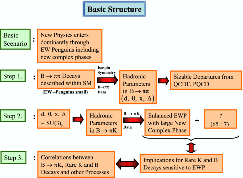
Figure 1: Outline of our strategy

A chart of the three steps in question is given in Fig. 1. Before going into the details it is important to emphasize that our strategy is valid both in the SM and all SM extensions in which NP enters predominantly through the EW penguin sector. This means that even if the presently observed deviations from the SM in the $B\to\pi K$ sector would diminish with improved data, our strategy would still be useful in correlating the phenomena in $B\to\pi\pi$, $B\to\pi K$ and rare $K$ and $B$ decays within the SM. If, on the other hand, the observed deviations from the SM in $B\to\pi\pi$ decays would not be attributed to the modification in hadron dynamics but to NP contributions, our approach should be properly generalized.

3 $B\to\pi\pi$ decays

The central quantities for our analysis of the $B\to\pi\pi$ decays are the ratios

$$R_{+-}^{\pi\pi} \equiv 2\left[\frac{\mbox{BR}(B^{+}\to\pi^{+}\pi^{0})+\mbox{BR}(B^{-}\to\pi^{-}\pi^{0})}{\mbox{BR}(B_{d}^{0}\to\pi^{+}\pi^{-})+\mbox{BR}(\bar{B}_{d}^{0}\to\pi^{+}\pi^{-})}\right]\frac{\tau_{B^{0}_{d}}}{\tau_{B^{+}}}$$ (1)

$$R_{00}^{\pi\pi} \equiv 2\left[\frac{\mbox{BR}(B_{d}^{0}\to\pi^{0}\pi^{0})+\mbox{BR}(\bar{B}_{d}^{0}\to\pi^{0}\pi^{0})}{\mbox{BR}(B_{d}^{0}\to\pi^{+}\pi^{-})+\mbox{BR}(\bar{B}_{d}^{0}\to\pi^{+}\pi^{-})}\right]$$ (2)

of the CP-averaged $B\to\pi\pi$ branching ratios, and the CP-violating observables provided by the time-dependent rate asymmetry

$$\frac{\Gamma(B^{0}_{d}(t)\to\pi^{+}\pi^{-})-\Gamma(\bar{B}^{0}_{d}(t)\to\pi^{+}\pi^{-})}{\Gamma(B^{0}_{d}(t)\to\pi^{+}\pi^{-})+\Gamma(\bar{B}^{0}_{d}(t)\to\pi^{+}\pi^{-})}$$ (3)

$$={\cal A}_{\rm CP}^{\rm dir}(B_{d}\to\pi^{+}\pi^{-})\cos(\Delta M_{d}t)+{\cal A}_{\rm CP}^{\rm mix}(B_{d}\to\pi^{+}\pi^{-})\sin(\Delta M_{d}t)\,.$$

The current status of the $B\to\pi\pi$ data together with the relevant references can be found in Table 1.

Quantity	Input	Exp. reference
$\mbox{BR}(B^{\pm}\to\pi^{\pm}\pi^{0})/10^{-6}$	$5.5\pm 0.6$	[?,?]
$\mbox{BR}(B_{d}\to\pi^{+}\pi^{-})/10^{-6}$	$4.6\pm 0.4$	[?,?]
$\mbox{BR}(B_{d}\to\pi^{0}\pi^{0})/10^{-6}$	$1.51\pm 0.28$	[?,?]
$R_{+-}^{\pi\pi}$	$2.20\pm 0.31$
$R_{00}^{\pi\pi}$	$0.67\pm 0.14$
${\cal A}_{\rm CP}^{\rm dir}(B_{d}\to\pi^{+}\pi^{-})$	$-0.37\pm 0.11$	[?,?]
${\cal A}_{\rm CP}^{\rm mix}(B_{d}\to\pi^{+}\pi^{-})$	$+0.61\pm 0.14$	[?,?]

Table 1: The current status of the $B\to\pi\pi$ input data for our strategy, with averages taken from [?]. For the evaluation of $R_{+-}^{\pi\pi}$, we have used the life-time ratio $\tau_{B^{+}}/\tau_{B^{0}_{d}}=1.086\pm 0.017$ [?].

The so-called “$B\to\pi\pi$ puzzle” is reflected in a surprisingly large value of $\mbox{BR}(B_{d}\to\pi^{0}\pi^{0})$ and a somewhat small value of $\mbox{BR}(B_{d}\to\pi^{+}\pi^{-})$, which results in large values of both $R_{00}^{\pi\pi}$ and $R_{+-}^{\pi\pi}$. For instance, the central values calculated within QCD factorization (QCDF) [?] give $R_{00}^{\pi\pi}=0.07$ and $R_{+-}^{\pi\pi}=1.24$ [?], although in the scenario “S4” of [?] values 0.2 and 2.0, respectively, can be obtained. As already pointed out in [?], these data indicate important non-factorizable contributions rather than NP effects, and can be perfectly accommodated in the SM. The same applies to the NP scenario considered in [?,?], in which the EW penguin contributions to $B\to\pi\pi$ are marginal.

In order to address this issue in explicit terms, we use the isospin symmetry to find

$$\sqrt{2}A(B^{+}\to\pi^{+}\pi^{0}) = -[\tilde{T}+\tilde{C}]=-[T+C]$$ (4)

$$A(B^{0}_{d}\to\pi^{+}\pi^{-}) = -[\tilde{T}+P]$$ (5)

$$\sqrt{2}A(B^{0}_{d}\to\pi^{0}\pi^{0}) = -[\tilde{C}-P].$$ (6)

The individual amplitudes of (4)–(6) can be expressed as

$$P = \lambda^{3}A({\cal P}_{t}-{\cal P}_{c})\equiv\lambda^{3}A{\cal P}_{tc}$$ (7)

$$\tilde{T} = \lambda^{3}AR_{b}e^{i\gamma}\left[{\cal T}-\left({\cal P}_{tu}-{\cal E}\right)\right]$$ (8)

$$\tilde{C} = \lambda^{3}AR_{b}e^{i\gamma}\left[{\cal C}+\left({\cal P}_{tu}-{\cal E}\right)\right],$$ (9)

where

$$\lambda\equiv|V_{us}|=0.2240\pm 0.0036,\quad A\equiv|V_{cb}|/\lambda^{2}=0.83\pm 0.02$$ (10)

are the usual parameters in the Wolfenstein expansion of the Cabibbo–Kobayashi–Maskawa (CKM) matrix [?,?],

$$R_{b}\equiv\sqrt{\bar{\rho}^{2}+\bar{\eta}^{2}}=\left(1-\frac{\lambda^{2}}{2}\right)\frac{1}{\lambda}\left|\frac{V_{ub}}{V_{cb}}\right|=0.37\pm 0.04$$ (11)

measures one side of the UT, the ${\cal P}_{q}$ describe the strong amplitudes of QCD penguins with internal $q$-quark exchanges ($q\in\{t,c,u\}$), including annihilation and exchange penguins, while ${\cal T}$ and ${\cal C}$ are the strong amplitudes of colour-allowed and colour-suppressed tree-diagram-like topologies, respectively, and ${\cal E}$ denotes the strong amplitude of an exchange topology. The amplitudes $\tilde{T}$ and $\tilde{C}$ differ from

$$T=\lambda^{3}AR_{b}e^{i\gamma}{\cal T},\quad C=\lambda^{3}AR_{b}e^{i\gamma}{\cal C}$$ (12)

through the $({\cal P}_{tu}-{\cal E})$ pieces, which may play an important rôle [?]. Note that these terms contain also the “GIM penguins” with internal up-quark exchanges, whereas their “charming penguin” counterparts enter in $P$ through ${\cal P}_{c}$, as can be seen in (7) [?,?,?,?].

In order to characterize the dynamics of the $B\to\pi\pi$ system, we introduce four hadronic parameters $d$, $\theta$, $x$ and $\Delta$ through

$$de^{i\theta}=-\left|\frac{P}{\tilde{T}}\right|e^{i(\delta_{P}-\delta_{\tilde{T}})}\,,\quad xe^{i\Delta}=\left|\frac{\tilde{C}}{\tilde{T}}\right|e^{i(\delta_{\tilde{C}}-\delta_{\tilde{T}})}\,,$$ (13)

with $\delta_{i}$ being strong phases. Using this parametrization, we have

$$R_{+-}^{\pi\pi}=F_{1}(d,\theta,x,\Delta;\gamma),\quad R_{00}^{\pi\pi}=F_{2}(d,\theta,x,\Delta;\gamma),$$ (14)

$${\cal A}_{\rm CP}^{\rm dir}(B_{d}\to\pi^{+}\pi^{-})=G_{1}(d,\theta;\gamma),\quad{\cal A}_{\rm CP}^{\rm mix}(B_{d}\to\pi^{+}\pi^{-})=G_{2}(d,\theta;\gamma,\phi_{d}),$$ (15)

with explicit expressions for $F_{1}$, $F_{2}$, $G_{1}$ and $G_{2}$ given in [?]. Taking then as the input

$$\gamma=(65\pm 7)^{\circ}\,,\quad\phi_{d}=2\beta=\left(46.5^{+3.2}_{-3.0}\right)^{\circ}$$ (16)

and the data for $R_{+-}^{\pi\pi}$, $R_{00}^{\pi\pi}$, ${\cal A}_{\rm CP}^{\rm dir}$ and ${\cal A}_{\rm CP}^{\rm mix}$ of Table 1, we obtain a set of four equations with the four unknowns $d$, $\theta$, $x$ and $\Delta$. Interestingly, as demonstrated in [?,?], a unique solution for these parameters can be found:

$$d=0.51^{+0.26}_{-0.20},\quad\theta=\left(140^{+14}_{-18}\right)^{\circ},\quad x=1.15^{+0.18}_{-0.16},\quad\Delta=-\left(59^{+19}_{-26}\right)^{\circ}.$$ (17)

The large values of the strong phases $\theta$ and $\Delta$ and the large values of $d$ and $x$ signal departures from the picture of QCDF. Going back to (8) and (9) we observe that these effects can be attributed to the enhancement of the $({\mathcal{P}}_{tu}-{\cal E})$ terms that in turn suppresses ${\tilde{T}}$ and enhances ${\tilde{C}}$. In this manner, $\mbox{BR}(B_{d}\to\pi^{+}\pi^{-})$ and $\mbox{BR}(B_{d}\to\pi^{0}\pi^{0})$ are suppressed and enhanced, respectively. Moreover, also a sizeable deviation of the “colour-suppression” parameter $a_{2}^{\pi\pi}e^{i\Delta_{2}^{\pi\pi}}\equiv{\cal C}_{\pi\pi}/{\cal T}_{\pi\pi}$ from its naive value around 0.25 is suggested by the data, with $0.5\mathrel{\hbox{\hbox to0.0pt{\hbox{\lower 4.0pt\hbox{$\sim$}}\hss}\hbox{$<$}}}a_{2}^{\pi\pi}\mathrel{\hbox{\hbox to0.0pt{\hbox{\lower 4.0pt\hbox{$\sim$}}\hss}\hbox{$<$}}}0.7$ and $\Delta_{2}^{\pi\pi}\sim 290^{\circ}$ [?].

With the hadronic parameters at hand, we can predict the direct and mixing-induced CP asymmetries of the $B_{d}\to\pi^{0}\pi^{0}$ channel. These predictions, while still subject to large uncertainties, have been confirmed by the most recent data. On the other hand, as illustrated in [?], a future precise measurement of ${\cal A}_{\rm CP}^{\rm dir}(B_{d}\to\pi^{0}\pi^{0})$ or ${\cal A}_{\rm CP}^{\rm mix}(B_{d}\to\pi^{0}\pi^{0})$ allows a theoretically clean determination of $\gamma$.

The large non-factorizable effects found in [?] have been discussed at length in [?,?], and have been confirmed in [?,?,?,?,?,?]. For the following sections, the most important outcome of this analysis are the values of the hadronic parameters $d$, $\theta$, $x$ and $\Delta$ in (17). These quantities will allow us – with the help of the $SU(3)$ flavour symmetry – to determine the corresponding hadronic parameters of the $B\to\pi K$ system.

4 $B\to\pi K$ decays

The key observables for our discussion are the following ratios:

$$R \equiv \left[\frac{\mbox{BR}(B_{d}^{0}\to\pi^{-}K^{+})+\mbox{BR}(\bar{B}_{d}^{0}\to\pi^{+}K^{-})}{\mbox{BR}(B^{+}\to\pi^{+}K^{0})+\mbox{BR}(B^{-}\to\pi^{-}\bar{K}^{0})}\right]\frac{\tau_{B^{+}}}{\tau_{B^{0}_{d}}}$$ (18)

$$R_{\rm c} \equiv 2\left[\frac{\mbox{BR}(B^{+}\to\pi^{0}K^{+})+\mbox{BR}(B^{-}\to\pi^{0}K^{-})}{\mbox{BR}(B^{+}\to\pi^{+}K^{0})+\mbox{BR}(B^{-}\to\pi^{-}\bar{K}^{0})}\right]$$ (19)

$$R_{\rm n} \equiv \frac{1}{2}\left[\frac{\mbox{BR}(B_{d}^{0}\to\pi^{-}K^{+})+\mbox{BR}(\bar{B}_{d}^{0}\to\pi^{+}K^{-})}{\mbox{BR}(B_{d}^{0}\to\pi^{0}K^{0})+\mbox{BR}(\bar{B}_{d}^{0}\to\pi^{0}\bar{K}^{0})}\right],$$ (20)

where the current status of the relevant branching ratios and the corresponding values of the $R_{i}$ is summarized in Table 2.

Quantity	Data	Exp. reference
$\mbox{BR}(B_{d}\to\pi^{\mp}K^{\pm})/10^{-6}$	$18.2\pm 0.8$	[?,?]
$\mbox{BR}(B^{\pm}\to\pi^{\pm}K)/10^{-6}$	$24.1\pm 1.3$	[?,?]
$\mbox{BR}(B^{\pm}\to\pi^{0}K^{\pm})/10^{-6}$	$12.1\pm 0.8$	[?,?]
$\mbox{BR}(B_{d}\to\pi^{0}K)/10^{-6}$	$11.5\pm 1.0$	[?,?]
$R$	$0.82\pm 0.06$	$0.91\pm 0.07$
$R_{\rm c}$	$1.00\pm 0.08$	$1.17\pm 0.12$
$R_{\rm n}$	$0.79\pm 0.08$	$0.76\pm 0.10$

Table 2: The current status of the CP-averaged $B\to\pi K$ branching ratios, with averages taken from [?]. We also give the values of the ratios $R$, $R_{\rm c}$ and $R_{\rm n}$ introduced in (18), (19) and (20), where $R$ refers again to $\tau_{B^{+}}/\tau_{B^{0}_{d}}=1.086\pm 0.017$ [?]. In the last column we also give the values of $R_{i}$ at the time of the analyses in [?,?].

The so-called “$B\to\pi K$ puzzle”, which was already pointed out in [?], is reflected in the small value of $R_{\rm n}$ that is significantly lower than $R_{\rm c}$. We will return to this below.

In order to analyze this issue, we neglect for simplicity the colour-suppressed EW penguins and use the $SU(3)$ flavour symmetry to find:

$$A(B^{0}_{d}\to\pi^{-}K^{+}) = P^{\prime}\left[1-re^{i\delta}e^{i\gamma}\right]$$ (21)

$$A(B^{\pm}_{d}\to\pi^{\pm}K^{0}) = -P^{\prime}$$ (22)

$$\sqrt{2}A(B^{+}\to\pi^{0}K^{+}) = P^{\prime}\left[1-\left(e^{i\gamma}-qe^{i\phi}\right)r_{\rm c}e^{i\delta_{\rm c}}\right]$$ (23)

$$\sqrt{2}A(B^{0}_{d}\to\pi^{0}K^{0}) = -P^{\prime}\left[1+\rho_{\rm n}e^{i\theta_{\rm n}}e^{i\gamma}-qe^{i\phi}r_{\rm c}e^{i\delta_{\rm c}}\right].$$ (24)

Here, $P^{\prime}$ is a QCD penguin amplitude that does not concern us as it cancels in the ratios $R_{i}$ and in the CP asymmetries considered. The parameters $r$, $\delta$, $\rho_{\rm n}$, $\theta_{\rm n}$, $r_{\rm c}$ and $\delta_{\rm c}$ are of hadronic origin. If they were considered as completely free, the predictive power of (21)–(24) would be rather low. Fortunately, using the $SU(3)$ flavor symmetry, they can be related to the parameters $d$, $\theta$, $x$ and $\Delta$ that we have determined in the previous section; explicit expressions can be found in [?]. In this manner, the values of $r$, $\delta$, $\rho_{\rm n}$, $\theta_{\rm n}$, $r_{\rm c}$ and $\delta_{\rm c}$ can be found. The specific numerical values for these parameters are not of particular interest here and can be found in [?]. It suffices to say that they also signal large non-factorizable hadronic effects.

The most important recent experimental result concerning the $B\to\pi K$ system is the observation of direct CP violation in $B_{d}\to\pi^{\mp}K^{\pm}$ decays [?,?]. This phenomenon is described by the following rate asymmetry:

$${\cal A}_{\rm CP}^{\rm dir}(B_{d}\to\pi^{\mp}K^{\pm})\equiv\frac{\mbox{BR}(B^{0}_{d}\to\pi^{-}K^{+})-\mbox{BR}(\bar{B}^{0}_{d}\to\pi^{+}K^{-})}{\mbox{BR}(B^{0}_{d}\to\pi^{-}K^{+})+\mbox{BR}(\bar{B}^{0}_{d}\to\pi^{+}K^{-})}=+0.113\pm 0.019,$$ (25)

where the numerical value is the average compiled in [?]. Using the values of $r$ and $\delta$ as determined above and (21), we obtain ${\cal A}_{\rm CP}^{\rm dir}(B_{d}\to\pi^{\mp}K^{\pm})=+0.127^{+0.102}_{-0.066}$, which is in nice accordance with the experimental result. In fact, we argued in our previous analysis [?], which implied $+0.140^{+0.139}_{-0.087}$ and was confronted with the experimental average $+0.095\pm 0.028$, that this CP asymmetry should go up. Following the lines of [?,?], we may determine the angle $\gamma$ of the UT by complementing the CP-violating $B_{d}\to\pi^{+}\pi^{-}$ observables with either the ratio of the CP-averaged branching ratios $\mbox{BR}(B_{d}\to\pi^{\mp}K^{\pm})$ and $\mbox{BR}(B_{d}\to\pi^{+}\pi^{-})$ or the direct CP-asymmetry ${\cal A}_{\rm CP}^{\rm dir}(B_{d}\to\pi^{\mp}K^{\pm})$. These avenues, where the latter is theoretically more favourable, yield the following results:

$$\left.\gamma\right|_{\rm BR}=\left(63.3\,^{+7.7}_{-11.1}\right)^{\circ},\quad\left.\gamma\right|_{{\cal A}_{\rm CP}^{\rm dir}}=\left(66.6\,^{+11.0}_{-11.1}\right)^{\circ},$$ (26)

which are nicely consistent with each other. Moreover, these ranges are in remarkable accordance with the SM picture, as can be seen in Fig. 2, where we compare these values of $\gamma$ with the UT fit performed in [?]. A similar extraction of $\gamma$ can be found in [?].

Apart from ${\cal A}_{\rm CP}^{\rm dir}(B_{d}\to\pi^{\mp}K^{\pm})$, two observables are left that are only marginally affected by EW penguins: the ratio $R$ introduced in (18) and the direct CP asymmetry of $B^{\pm}\to\pi^{\pm}K$ modes. These observables may be affected by another hadronic parameter $\rho_{\rm c}e^{i\theta_{\rm c}}$, which is expected to play a minor rôle and was neglected in (22) and (23). In this approximation, the direct $B^{\pm}\to\pi^{\pm}K$ CP asymmetry vanishes – in accordance with the experimental value of $+0.020\pm 0.034$ – and the new experimental value of $R=0.82\pm 0.06$, which is on the lower side, can be converted into $\gamma\leq(64.9^{+4.8}_{-4.2})^{\circ}$ with the help of the bound derived in [?]. On the other hand, if we use the values of $r$ and $\delta$ as determined above, we obtain

$$R=0.943^{+0.028}_{-0.021},$$ (27)

which is sizeably larger than the experimental value. The nice agreement of the data with our prediction of ${\cal A}_{\rm CP}^{\rm dir}(B_{d}\to\pi^{\mp}K^{\pm})$, which is independent of $\rho_{\rm c}$, suggests that this parameter is actually the origin of the deviation of $R$. In fact, as discussed in detail in [?], the emerging signal for $B^{\pm}\to K^{\pm}K$ decays, which provide direct access to $\rho_{\rm c}$, shows that our value of $R$ in (27) is shifted towards the experimental value through this parameter, thereby essentially resolving this small discrepancy.

It is imporant to emphasize that we could accommodate all the $B\to\pi\pi$ and $B\to\pi K$ data so far nicely in the SM. Moreover, as discussed in detail in [?,?], there are also a couple of internal consistency checks of our working assumptions, which work impressively well within the current uncertainties.

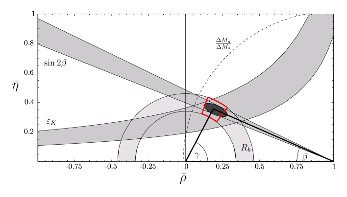
Figure 2: Illustration of the value of $\gamma$ following from the CP-violating $B_{d}\to\pi^{+}\pi^{-}$ observables and the data for the $B_{d}\to\pi^{\mp}K^{\pm}$ decays in the $\bar{\rho}$–$\bar{\eta}$ plane and comparison with the other constraints for the UT, as discussed in [?]. The shaded dark ellipse is the result of the UT fit, while the quadrangle corresponds to the second value of $\left.\gamma\right|_{\rm BR}$ in (26) and the $R_{b}$ constraint.

Let us now turn our attention to (23) and (24). The only variables in these formulae that we did not discuss so far are the parameters $q$ and $\phi$ that parametrize the EW penguin sector. The fact that EW penguins cannot be neglected here is related to the simple fact that a $\pi^{0}$ meson can be emitted directly in these colour-allowed EW penguin topologies, while the corresponding emission with the help of QCD penguins is colour-suppressed. In the SM, the parameters $q$ and $\phi$ can be determined with the help of the $SU(3)$ flavour symmetry of strong interactions [?], yielding

$$q=0.69\times\left[\frac{0.086}{|V_{ub}/V_{cb}|}\right],\qquad\phi=0^{\circ}.$$ (28)

In this manner, predictions for $R_{\rm c}$ and $R_{\rm n}$ can be made [?,?], which read as follows [?]:

$$\left.R_{\rm c}\right|_{\rm SM}=1.14\pm 0.05,\,\quad\left.R_{\rm n}\right|_{\rm SM}=1.11^{+0.04}_{-0.05}\,.$$ (29)

Comparing with the experimental results in Table 2, we observe that there is only a marginal discrepancy in the case of $R_{\rm c}$, whereas the value of $R_{\rm n}$ in (29) is definetely too large. The “$B\ \to\pi K$” puzzle is seen here in explicit terms.

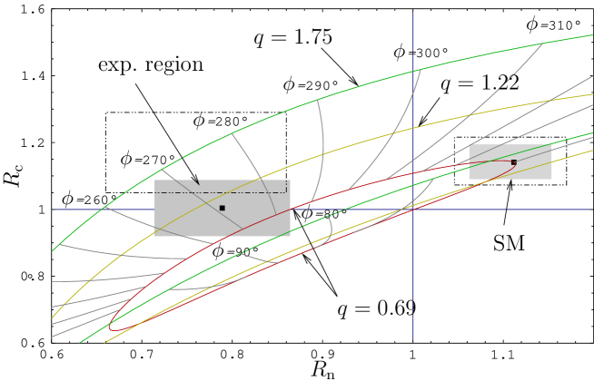
Figure 3: The situation in the $R_{\rm n}$–$R_{\rm c}$ plane. We show contours for values of $q=0.69$, $q=1.22$ and $q=1.75$, with $\phi\in[0^{\circ},360^{\circ}]$. The experimental ranges for $R_{\rm c}$ and $R_{\rm n}$ and those predicted in the SM are indicated in grey, the dashed lines serve as a reminder of the corresponding ranges in [?].

The disagreement of the SM with the data can be resolved in the scenario of enhanced EW penguins carrying a non-vanishing phase $\phi$. Indeed, using the measured values of $R_{\rm n}$ and $R_{\rm c}$, we find [?]:

$$q=1.08\,^{+0.81}_{-0.73},\quad\,\phi=-(88.8^{+13.7}_{-19.0})^{\circ}\,.$$ (30)

We observe that – while $q$ is consistent with the SM estimate within the errors – the large phase $\phi$ is a spectacular signal of possible NP contributions. It is useful to consider the $R_{\rm n}$–$R_{\rm c}$ plane, as we have done in Fig. 3. There we show contours corresponding to different values of $q$, and indicate the experimental and SM ranges. Following [?], we choose the values of $q=0.69$, $1.22$ and $1.75$, where the latter reproduced the central values of $R_{\rm c}$ and $R_{\rm n}$ in our previous analysis [?,?]. The central values for the SM prediction have hardly moved, while their uncertainties have been reduced a bit. On the other hand, the central experimental values of $R_{\rm c}$ and $R_{\rm n}$ have moved in such a way that $q$ decreased, while the weak phase $\phi$ remains around $-90^{\circ}$.

We close this section with a list of predictions for the CP asymmetries in the $B\to\pi\pi$ and $B\to\pi K$ systems, which are summarized in Table 3.

Quantity	Our Prediction	Experiment
${\cal A}_{\rm CP}^{\rm dir}(B_{d}\!\to\!\pi^{0}\pi^{0})$	$-0.28^{+0.37}_{-0.21}$	$-0.28\pm 0.39$
${\cal A}_{\rm CP}^{\rm mix}(B_{d}\!\to\!\pi^{0}\pi^{0})$	$-0.63^{+0.45}_{-0.41}$	$-0.48_{-0.40}^{+0.48}$
${\cal A}_{\rm CP}^{\rm dir}(B_{d}\!\to\!\pi^{\mp}K^{\pm})$	$0.127^{+0.102}_{-0.066}$	$0.113\pm 0.019$
${\cal A}_{\rm CP}^{\rm dir}(B^{\pm}\!\to\!\pi^{0}K^{\pm})$	$0.10^{+0.25}_{-0.19}$	$-0.04\pm 0.04$
${\cal A}_{\rm CP}^{\rm dir}(B_{d}\!\to\!\pi^{0}K_{\rm S})$	$0.01^{+0.15}_{-0.18}$	$0.09\pm 0.14$
${\cal A}_{\rm CP}^{\rm mix}(B_{d}\!\to\!\pi^{0}K_{\rm S})$	$-0.98^{+0.04}_{-0.02}$	$-0.34^{+0.29}_{-0.27}$

Table 3: Compilation of our predictions for the CP-violating $B\to\pi\pi$, $\pi K$ asymmetries.

5 Implications for Rare $K$ and $B$ Decays

The rates for rare $K$ and $B$ decays are sensitive functions of the EW penguin contributions. In a simple scenario in which NP enters the EW penguin sector predominantly through $Z^{0}$ penguins and the local operators in the effective Hamiltonians for rare decays are the same as in the SM, there is a strict relation [?,?,?] between the EW penguin effects in the $B\to\pi K$ system and the corresponding effects in rare $K$ and $B$ decays. Denoting by $C$ the $Z^{0}$-penguin function, we find

$$C=|C|e^{i\theta_{C}}=2.35\bar{q}e^{i\phi}-0.82,\qquad\bar{q}=q\left|\frac{V_{ub}/V_{cb}}{0.086}\right|\,.$$ (31)

In turn, the functions $X$, $Y$, $Z$ that govern rare decays in the scenarios in question become explicit functions of $q$ and $\phi$:

$$X=|X|e^{i\theta_{X}} = 2.35\bar{q}e^{i\phi}-0.09,$$ (32)

$$Y=|Y|e^{i\theta_{Y}} = 2.35\bar{q}e^{i\phi}-0.64,$$ (33)

$$Z=|Z|e^{i\theta_{Z}} = 2.35\bar{q}e^{i\phi}-0.94.$$ (34)

If the phase $\phi$ was zero (the case considered in [?]), the functions $X$, $Y$, $Z$ would remain to be real quantities as in the SM but the enhancement of $q$ would imply enhancements of $X$, $Y$, $Z$ as well. As in the scenario considered $X$, $Y$, $Z$ are not independent of one another, it is sufficient to constrain one of them from rare decays in order to see whether the enhancement of $q$ is consistent with the existing data on rare decays. It turns out that the data on inclusive $B\to X_{s}l^{+}l^{-}$ decays [?,?] are presently most powerful to constrain $X$, $Y$, $Z$, but due to significant experimental errors and theoretical uncertainties these bounds are only approximate. Typically, one finds $X$, $Y$, $Z$ to be at most $2.2$ to be compared with $X\approx 1.5$, $Y\approx 1.0$, $Z\approx 0.7$, in the SM, thereby leaving still some room for NP contributions.

Now, $X$ governs decays with $\nu\bar{\nu}$ in the final state like $K\to\pi\nu\bar{\nu}$, $Y$ governs decays with $l^{+}l^{-}$ in the final state like $B_{s,d}\to\mu^{+}\mu^{-}$, $K_{\rm L}\to\pi^{0}l^{+}l^{-}$ and $B\to X_{s}l^{+}l^{-}$, while $Z$ is relevant for $K_{\rm L}\to\pi^{0}l^{+}l^{-}$, $B\to X_{s}l^{+}l^{-}$ and in particular for $\varepsilon^{\prime}/\varepsilon$. In the situation with $\phi=0^{\circ}$ there is clearly room for sizable departures in rare decay rates from the SM expectation [?], but in particular the branching ratios for $K^{+}\to\pi^{+}\nu\bar{\nu}$ and $K_{\rm L}\to\pi^{0}\nu\bar{\nu}$ are only enhanced by at most factors of $2$–$2.5$ as in other models with minimal flavour violation (MFV) [?,?] in which no new phases beyond the KM phase are present.

The situation changes drastically if $\phi$ is required to be non-zero, in particular when its value is in the ball park of $-90^{\circ}$ as found in the previous section. In this case, $X$, $Y$ and $Z$ become complex quantities, as seen in (32)–(34), with the phases $\theta_{i}$ in the ball park of $-90^{\circ}$ [?,?]:

$$\theta_{X}=-(86\pm 12)^{\circ},\qquad\theta_{Y}=-(100\pm 12)^{\circ},\qquad\theta_{Z}=-(108\pm 12)^{\circ}.$$ (35)

Actually, the data for the $B\to\pi K$ decays used in our first analysis [?] were such that $q=1.75^{+1.27}_{-0.99}$ and $\phi=-(85^{+11}_{-14})$ were required, implying $|X|\approx|Y|\approx|Z|\approx 4.3^{+3.0}_{-2.4}$, barely consistent with the data. Choosing $|Y|=2.2$ as high as possible but still consistent with the data on $B\to X_{s}l^{+}l^{-}$ , we found

$$\bar{q}=0.92^{+0.07}_{-0.05}\,,\qquad\phi=-(85^{+11}_{-14})^{\circ}\,,$$ (36)

which has been already taken into account in obtaining the values in (35). This in turn made us expect that the experimental values $R_{\rm c}=1.17\pm 0.12$ and $R_{\rm n}=0.76\pm 0.10$ known at the time of the analysis in [?] could change (see Fig. 3) once the data improve. Indeed, our expectation [?],

$$R_{\rm c}=1.00^{+0.12}_{-0.08}\qquad R_{\rm n}=0.82^{+0.12}_{-0.11},$$ (37)

has been confirmed by the most recent results in Table 2, making the overall description of the $B\to\pi\pi$, $B\to\pi K$ and rare decays within our approach significantly better with respect to our previous analysis.

There is a characteristic pattern of modifications of branching ratios relative to the case of $\phi=0^{\circ}$ and $\theta_{i}=0^{\circ}$:

• The branching ratios proportional to $|X|^{2}$, like $\mbox{BR}(B\to X_{s}\nu\bar{\nu})$, and $|Y|^{2}$, like $\mbox{BR}(B_{d,s}\to\mu^{+}\mu^{-})$, remain unchanged relative to the case $\phi=0^{\circ}$, still exhibiting enhancements of roughly $2$ and $5$, respectively, over the SM expectations.

• In CP-conserving transitions in which in addition to top-like contributions also charm contribution plays some rôle, the constructive interference between top and charm contributions in the SM becomes destructive, thereby compensating for the enhancements of $X$, $Y$ and $Z$. In particular, $\mbox{BR}(K^{+}\to\pi^{+}\nu\bar{\nu})$ turns out to be rather close to the SM estimates, and the short-distance part of $\mbox{BR}(K_{\rm L}\to\mu^{+}\mu^{-})$ is even smaller than in the SM.

• Not surprisingly, the most spectacular impact of large phases $\theta_{i}$ is seen in CP-violating quantities sensitive to EW penguins.

In particular, one finds [?,?]

$$\frac{\mbox{BR}(K_{\rm L}\rightarrow\pi^{0}\nu\bar{\nu})}{\mbox{BR}(K_{\rm L}\rightarrow\pi^{0}\nu\bar{\nu})_{\rm SM}}=\left|\frac{X}{X_{\rm SM}}\right|^{2}\left[\frac{\sin(\beta-\theta_{X})}{\sin(\beta)}\right]^{2},$$ (38)

with the two factors on the right-hand side in the ball park of $2$ and $5$, respectively. Consequently, $\mbox{BR}(K_{\rm L}\rightarrow\pi^{0}\nu\bar{\nu})$ can be enhanced over the SM prediction even by an order of magnitude and is expected to be roughly by a factor of $4$ larger than $\mbox{BR}(K^{+}\rightarrow\pi^{+}\nu\bar{\nu})$. In the SM and most MFV models the pattern is totally different with $\mbox{BR}(K_{\rm L}\rightarrow\pi^{0}\nu\bar{\nu})$ smaller than $\mbox{BR}(K^{+}\rightarrow\pi^{+}\nu\bar{\nu})$ by a factor of $2$–$3$ [?,?,?]. On the other hand a recent analysis shows that a pattern of $BR(K\to\pi\nu\bar{\nu})$ expected in our NP scenario can be obtained in a general MSSM [?].

We note that $\mbox{BR}(K_{\rm L}\rightarrow\pi^{0}\nu\bar{\nu})$ is predicted to be rather close to its model-independent upper bound [?]

$$\mbox{BR}(K_{\rm L}\rightarrow\pi^{0}\nu\bar{\nu})\leq 4.4\,\mbox{BR}(K^{+}\rightarrow\pi^{+}\nu\bar{\nu}).$$ (39)

Moreover, another spectacular implication of these findings is a strong violation of the relation [?]

$$(\sin 2\beta)_{\pi\nu\bar{\nu}}=(\sin 2\beta)_{\psi K_{\rm S}},$$ (40)

which is valid in the SM and any model with MFV. Indeed, we find [?,?]

$$(\sin 2\beta)_{\pi\nu\bar{\nu}}=\sin 2(\beta-\theta_{X})=-(0.69^{+0.23}_{-0.41}),$$ (41)

in striking disagreement with $(\sin 2\beta)_{\psi K_{\rm S}}=0.725\pm 0.037$.

Even if eventually the departures from the SM and MFV pictures could turn out to be smaller than estimated here, finding $\mbox{BR}(K_{\rm L}\rightarrow\pi^{0}\nu\bar{\nu})$ to be larger than $\mbox{BR}(K^{+}\rightarrow\pi^{+}\nu\bar{\nu})$ would be a clear signal of new complex phases at work. For a more general discussion of the $K\to\pi\nu\bar{\nu}$ decays beyond the SM, see [?].

Similarly, as seen in Table 4, interesting enhancements are found in $K_{\rm L}\to\pi^{0}l^{+}l^{-}$ and the forward–backward CP asymmetry in $B\to X_{s}l^{+}l^{-}$ as discussed in [?].

Decay	SM prediction	Our scenario	Exp. bound  (90% C.L.)
$K^{+}\to\pi^{+}\bar{\nu}\nu$	$(7.8\pm 1.2)\cdot 10^{-11}$	$(7.5\pm 2.1)\cdot 10^{-11}$	$(14.7^{+13.0}_{-8.9})\cdot 10^{-11}$ [?]
$K_{\rm L}\to\pi^{0}\bar{\nu}\nu$	$(3.0\pm 0.6)\cdot 10^{-11}$	$(3.1\pm 1.0)\cdot 10^{-10}$	$<5.9\cdot 10^{-7}$ [?]
$K_{\rm L}\to\pi^{0}e^{+}e^{-}$	$(3.7^{+1.1}_{-0.9})\cdot 10^{-11}$	$(9.0\pm 1.6)\cdot 10^{-11}$	$<2.8\cdot 10^{-10}$ [?]
$K_{\rm L}\to\pi^{0}\mu^{+}\mu^{-}$	$(1.5\pm 0.3)\cdot 10^{-11}$	$(4.3\pm 0.7)\cdot 10^{-11}$	$<3.8\cdot 10^{-10}$ [?]
$B\to X_{s}\bar{\nu}\nu$	$(3.5\pm 0.5)\cdot 10^{-5}$	$\approx 7\cdot 10^{-5}$	$<6.4\cdot 10^{-4}$ [?]
$B_{s}\to\mu^{+}\mu^{-}$	$(3.42\pm 0.53)\cdot 10^{-9}$	$\approx 17\cdot 10^{-9}$	$<5.0\cdot 10^{-7}$ [?]

Table 4: Predictions for various rare decays in the scenario considered compared with the SM expectations and experimental bounds. For a theoretical update on $K_{\rm L}\to\pi^{0}e^{+}e^{-}$ and a discussion of $K_{\rm L}\to\pi^{0}\mu^{+}\mu^{-}$, see [?].

As emphasized above, the new data on $B\to\pi K$ improved the overall description of $B\to\pi\pi$, $B\to\pi K$ and rare decays within our approach. But, as the rare decay constraint from $B\to X_{s}l^{+}l^{-}$ has already been taken into account in [?], there is essentially no impact of these new data on our predictions for rare decays that we presented in [?]. In fact, as the central value of $q$ found in the previous section is still on the high side from the point of view of rare decays (compare (30) with (36)), we expect that $R_{\rm c}$ and $R_{\rm n}$ will still slightly move towards each other, when the data improve in the future. However, the most interesting question is whether the large negative values of $\phi$ and $\theta_{i}$ will be reinforced by the future more accurate data. This would be a very spectacular signal of NP!

6 Outlook

We have summarized our strategy for analyzing $B\to\pi\pi$, $B\to\pi K$ decays and rare $K$ and $B$ decays. Within a simple NP scenario of enhanced CP-violating EW penguins considered by us, the NP contributions enter significantly only in certain $B\to\pi K$ decays and rare $K$ and $B$ decays, while the $B\to\pi\pi$ system is practically unaffected by these contributions and can be described within the SM. The confrontation of our strategy with the most recent data on $B\to\pi\pi$ and $B\to\pi K$ modes from the BaBar and Belle collaborations is very encouraging. In particular, our earlier predictions for the direct CP asymmetries of $B_{d}\to\pi^{0}\pi^{0}$ and $B_{d}\to\pi^{\mp}K^{\pm}$ have been confirmed within the theoretical and experimental uncertainties, and the shift in the experimental values of $R_{\rm c}$ and $R_{\rm n}$ took place as expected.

It will be exciting to follow the experimental progress on $B\to\pi\pi$ and $B\to\pi K$ decays and the corresponding efforts in rare decays. In particular, new messages from BaBar and Belle that the present central values of $R_{\rm c}$ and $R_{\rm n}$ have been confirmed at a high confidence level, a slight increase of $R$ and a message from KEK [?] in the next two years that the decay $K_{\rm L}\to\pi^{0}\nu\bar{\nu}$ has been observed would give a strong support to the NP scenario considered here.

Acknowledgments
The work presented here was supported in part by the German Bundesministerium für Bildung und Forschung under the contract 05HT4WOA/3.

References

• [1] A.J. Buras, R. Fleischer, S. Recksiegel and F. Schwab, Phys. Rev. Lett. 92 (2004) 101804.
• [2] A.J. Buras, R. Fleischer, S. Recksiegel and F. Schwab, Nucl. Phys. B697 (2004) 133.
• [3] A. J. Buras, R. Fleischer, S. Recksiegel and F. Schwab, hep-ph/0410407.
• [4] A.J. Buras and L. Silvestrini, Nucl. Phys. B546 (1999) 299.
• [5] A.J. Buras, A. Romanino and L. Silvestrini, Nucl. Phys. B520 (1998) 3.
• [6] A.J. Buras, G. Colangelo, G. Isidori, A. Romanino and L. Silvestrini, Nucl. Phys. B566 (2000) 3.
• [7] G. Buchalla, G. Hiller and G. Isidori, Phys. Rev. D63 (2001) 014015;
D. Atwood and G. Hiller, LMU-09-03 [hep-ph/0307251].
• [8] B. Aubert et al.  [BaBar Collaboration], BABAR-CONF-04/035 [hep-ex/0408081].
• [9] Y. Chao et al. [Belle Collaboration], Phys. Rev. D69 (2004) 111102.
• [10] B. Aubert et al. [BABAR Collaboration], Phys. Rev. Lett. 89 (2002) 281802.
• [11] K. Abe et al.  [Belle Collaboration], BELLE-CONF-0406 [hep-ex/0408101].
• [12] B. Aubert et al. [BaBar Collaboration], BABAR-CONF-04/047 [hep-ex/0408089].
• [13] K. Abe et al. [Belle Collaboration], Phys. Rev. Lett. 93 (2004) 021601.
• [14] Heavy Flavour Averaging Group, http://www.slac.stanford.edu/xorg/hfag/.
• [15] S. Eidelman et al. [Particle Data Group], Phys. Lett. B592 (2004) 1.
• [16] M. Beneke, G. Buchalla, M. Neubert and C. T. Sachrajda, Phys. Rev. Lett.  83 (1999) 1914;
M. Beneke, G. Buchalla, M. Neubert and C. T. Sachrajda, Nucl. Phys. B  591 (2000) 313.
• [17] M. Beneke and M. Neubert, Nucl. Phys. B675 (2003) 333.
• [18] L. Wolfenstein, Phys. Rev. Lett. 51 (1983) 1945.
• [19] A.J. Buras, M.E. Lautenbacher and G. Ostermaier, Phys. Rev. D50 (1994) 3433.
• [20] A.J. Buras and R. Fleischer, Phys. Lett. B341 (1995) 379.
• [21] M. Ciuchini, E. Franco, G. Martinelli, L. Silvestrini, Nucl. Phys. B501 (1997) 271;
C. Isola, M. Ladisa, G. Nardulli, T.N. Pham and P. Santorelli, Phys. Rev. D64 (2001) 014029 and D65 (2002) 094005;
M. Ciuchini, E. Franco, G. Martinelli, M. Pierini and L. Silvestrini, Phys. Lett. B515 (2001) 33.
• [22] A.J. Buras, R. Fleischer and T. Mannel, Nucl. Phys. B533 (1998) 3.
• [23] C.W. Bauer, D. Pirjol, I.Z. Rothstein and I.W. Stewart, hep-ph/0401188.
• [24] R. Fleischer and S. Recksiegel, Eur. Phys. J. C (2004), Online First, DOI: 10.1140/epjc/s2004-02023-0 (hep-ph/0408016).
• [25] A. Ali, E. Lunghi and A.Y. Parkhomenko, Eur. Phys. J. C36 (2004) 183.
• [26] C.W. Chiang, M. Gronau, J.L. Rosner and D.A. Suprun, Phys. Rev. D70 (2004) 034020.
• [27] X. G. He and B. H. J. McKellar, hep-ph/0410098.
• [28] C. W. Bauer and D. Pirjol, Phys. Lett. B 604 (2004) 183.
• [29] T. Feldmann and T. Hurth, hep-ph/0408188.
• [30] B. Aubert et al. [BaBar Collaboration], BABAR-CONF-04/044 [hep-ex/0408080].
• [31] B. Aubert et al. [BaBar Collaboration], BABAR-CONF-04/30 [hep-ex/0408062].
• [32] A.J. Buras and R. Fleischer, Eur. Phys. J. C16 (2000) 97.
• [33] B. Aubert et al.  [BaBar Collaboration], Phys. Rev. Lett. 93 (2004) 131801.
• [34] Y. Chao et al.  [Belle Collaboration], Phys. Rev. Lett. 93 (2004) 191802.
• [35] R. Fleischer, Eur. Phys. J. C16 (2000) 87.
• [36] R. Fleischer and J. Matias, Phys. Rev. D66 (2002) 054009.
• [37] A.J. Buras, F. Schwab and S. Uhlig, TUM-HEP-547 [hep-ph/0405132].
• [38] Y. L. Wu and Y. F. Zhou, hep-ph/0409221.
• [39] R. Fleischer and T. Mannel, Phys. Rev. D57 (1998) 2752.
• [40] M. Neubert and J.L. Rosner, Phys. Lett. B441 (1998) 403; Phys. Rev. Lett. 81 (1998) 5076.
• [41] V. Barger, C. W. Chiang, P. Langacker and H. S. Lee, Phys. Lett.B598, (2004) 218
• [42] A.J. Buras, R. Fleischer, S. Recksiegel and F. Schwab, Eur. Phys. J. C32 (2003) 45.
• [43] J. Kaneko et al. [Belle Collaboration], Phys. Rev. Lett. 90 (2003) 021801
• [44] K. Abe et al. [Belle Collaboration], hep-ex/0408119.
• [45] A. J. Buras, P. Gambino, M. Gorbahn, S. Jäger and L. Silvestrini, Phys. Lett.B500 (2001) 161
• [46] G. D’Ambrosio, G. F. Giudice, G. Isidori and A. Strumia, Nucl. Phys. B645 (2002) 155
• [47] A.J. Buras and R. Fleischer, Phys. Rev. D64 (2001) 115010.
• [48] G. Buchalla and A.J. Buras, Phys. Lett. B333 (1994) 221, Phys. Rev. D54 (1996) 6782.
• [49] A. J. Buras, T. Ewerth, S. Jäger and J. Rosiek, hep-ph/0408142.
• [50] Y. Grossman and Y. Nir, Phys. Lett. B398 (1997) 163.
• [51] V. V. Anisimovsky et al. [E949 Collaboration], Phys. Rev. Lett. 93 (2004) 031801.
• [52] A. Alavi-Harati et al. [The E799-II/KTeV Collaboration], Phys. Rev. D61 (2000) 072006.
• [53] A. Alavi-Harati et al. [KTeV Collaboration], Phys. Rev. Lett. 93 (2004) 021805.
• [54] A. Alavi-Harati et al. [KTeV Collaboration], Phys. Rev. Lett. 84 (2000) 5279.
• [55] R. Barate et al. [ALEPH Collaboration], Eur. Phys. J. C19 (2001) 213.
• [56] V. M. Abazov [D0 Collaboration], FERMILAB-PUB-04-215-E [hep-ex/0410039].
• [57] G. Isidori, C. Smith and R. Unterdorfer, Eur. Phys. J. C36 (2004) 57.
• [58] J-PARC, http://www-ps.kek.jp/jhf-np/LOIlist/LOIlist.html