The common belief that the lightest supersymmetric particle (LSP) might be a neutralino, providing also the main Dark Matter (DM) component, calls for maximal detail in the study of the neutralino properties. Motivated by this, we consider the direct production of a single neutralino $\tilde{\chi}^{0}_{i}$ at a high/energy hadron collider, focusing on the $\tilde{\chi}^{0}_{1}$ and $\tilde{\chi}^{0}_{2}$ cases. At Born level, the relevant subprocesses are $q\bar{q}\to\tilde{\chi}^{0}_{i}\tilde{g}$, $gq\to\tilde{\chi}^{0}_{i}\tilde{q}_{L,R}$ and $q\bar{q}^{\prime}\to\tilde{\chi}^{0}_{i}\tilde{\chi}^{\pm}_{j}$; while at 1-loop, apart from radiative corrections to these processes, we consider also $gg\to\tilde{\chi}^{0}_{i}\tilde{g}$, for which a numerical code named PLATONgluino is released. The relative importance of these channels turns out to be extremely model dependent. Combining these results with an analogous study of the direct $\tilde{\chi}^{0}_{i}\tilde{\chi}^{0}_{j}$ pair production, should help in testing the SUSY models and the Dark Matter assignment.

PACS numbers: 12.15.-y, 12.15.Lk, 13.75.Cs, 14.80.Ly

1 Introduction

The lightest neutralino state, $\tilde{\chi}^{0}_{1}$, is often assumed to be the Lightest Supersymmetric Particle (LSP) [1]. As such it is also a candidate for the origin of Dark Matter (DM) [2]. This assumption has of course to be verified though, by analyzing the results or constraints reached by experiments trying to detect Dark Matter through direct or indirect methods [3, 4].

However, even in the minimal MSSM version of the SUSY models, the large parameter space induces great uncertainties in the neutralino properties. So to check the consistency of the DM idea, it is essential to establish the neutralino properties through production at high energy hadron and lepton colliders. The first such possibility of neutralino production, will probably be through cascades at the CERN LHC [5, 6]. But precious additional independent information from LHC could also be obtained by studying the smaller signals of the direct ($\tilde{\chi}^{0}_{i}\tilde{\chi}^{0}_{j}$) pair production, as well as the production in association with other sparticles in processes as $(\tilde{\chi}^{0}_{i}\tilde{g})$, ($\tilde{\chi}^{0}_{i}\tilde{q}_{L,R}$) or ($\tilde{\chi}^{0}_{i}\tilde{\chi}^{\pm}_{j}$). When the LC collider, will finally be built, a wealth of additional information will become accessible [7].

Studies of the pure QCD effects to these channels at LO and NLO have already appeared [8, 9]. A recent summary can be found in [10], where the results of a NLO QCD computation are presented for various processes including neutralino production in association with a gluino, squark, slepton, chargino, or another neutralino. The overall conclusion of these computations is that at the LHC range, the pure QCD soft and collinear corrections always increase the LO cross section by an amount which, depending on the subprocess c.m. energy and the masses of the particles involved, lies in the range of 10% to 40%.

Also important at LHC though, turn out to be the leading and subleading 1-loop logarithmic (LL) electroweak (EW) corrections. Particularly for processes characterized by non-vanishing Born contributions, such effects show a largely universal structure with the leading $\ln^{2}(\hat{s})$-terms solely determined by the couplings of the known gauge bosons $(W^{\pm},Z,\gamma)$ to the external particles of the process; which in turn are fixed completely by their quantum numbers. The situation is different for the subleading single-$\ln(\hat{s})$ terms though, which depend on the couplings and masses of all virtual particles, gauge or non-gauge, shaping up the underlying dynamics [11, 12, 13, 9]. Thus, depending on whether SUSY is ”near by” with all MSSM sparticles below the TeV range, or some of the sparticles are very heavy, or even that the pure simple SM model stays correct till very high scales, will only affect the subleading single $\ln(\hat{s})$-terms [11, 13, 14].

The most striking characteristic when comparing these EW corrections to the aforementioned pure QCD ones, is that they are of roughly similar magnitude, but have opposite sign [11, 12, 13, 14].

Particularly for the subprocess $q\bar{q}\to\tilde{\chi}^{0}_{i}\tilde{\chi}^{0}_{j}$ contributing to the neutralino-pair production, these effects have been studied in [15], where the calculation of the pure 1-loop process $gg\to\tilde{\chi}^{0}_{i}\tilde{\chi}^{0}_{j}$ was also included. If the masses of the squarks of the 1rst and 2nd family turn out to be very heavy, it might happen at LHC, that the $gg\to\tilde{\chi}^{0}_{i}\tilde{\chi}^{0}_{j}$ contribution is comparable to that of the LO process $q\bar{q}\to\tilde{\chi}^{0}_{i}\tilde{\chi}^{0}_{j}$, particularly at low invariant masses where the gluon flux is very large.

Additional information on neutralinos in a hadron collider could be obtained from the single neutralino production triggered by the subprocesses:

$$~{}~{}q\bar{q}\to\tilde{\chi}^{0}_{i}\tilde{g}~{}~{},~{}~{}gg\to\tilde{\chi}^{0}_{i}\tilde{g}~{}~{},~{}~{}gq\to\tilde{\chi}^{0}_{i}\tilde{q}_{L,R}~{}~{},~{}~{}q\bar{q}^{\prime}\to\tilde{\chi}^{0}_{i}\tilde{\chi}^{\pm}_{j}~{}~{},~{}~{}$$ (1)

where the indices $(i,j)$ now enumerate the neutralino and chargino respectively. The aim of the present paper is to study the physical consequences of these subprocesses using the same procedure as in [15]. Since different particles are involved in each of them, their combined study is sensitive to different aspects of the underlying model.

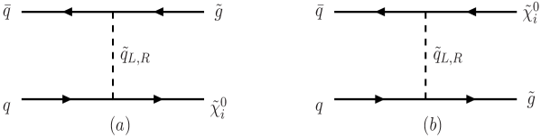
Figure 1: Born diagrams for $q\bar{q}\to\tilde{\chi}^{0}_{i}\tilde{g}$

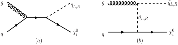
Figure 2: Born diagrams for $qg\to\tilde{\chi}^{0}_{i}\tilde{q}_{(L,R)}$.

For the first, third and fourth of the subprocesses in (1), this model sensitivity arises already at the Born level mainly caused by the (gaugino-higgsino) mixing matrices multiplying the basic gaugino and higgsino couplings. The relevant diagrams are shown in Figs.1-3 . This model sensitivity is further enhanced when including also the leading logarithmic part of the 1-loop corrections, calculated by following the procedure of [11]. Thus, rather simple expressions for the amplitudes of these processes are reached, which apart from being very sensitive to the physical dynamics, should also be quite adequate for LHC energies and accuracies.

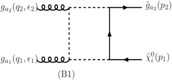
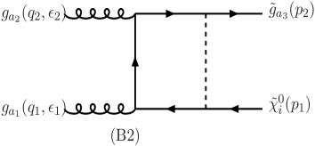
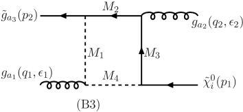
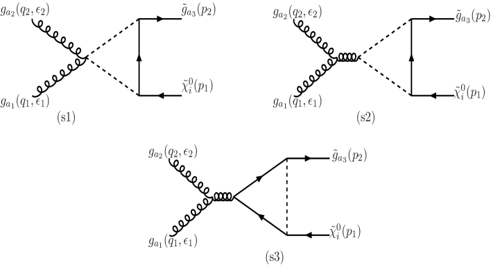
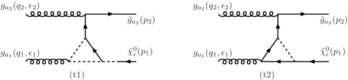
Figure 4: Feynman diagrams for $gg\to\tilde{\chi}^{0}_{i}\tilde{g}$. The full, broken and wavy lines respectively denote fermions, scalars and gluons.

Further model sensitivity is induced in the case of $\tilde{\chi}^{0}_{i}\tilde{g}$ production, by the contribution of the genuine 1-loop subprocess $gg\to\tilde{\chi}^{0}_{i}\tilde{g}$. The generic form of the relevant diagrams is shown in Fig.4. On the basis of these, a numerical Fortran code called PLATONgluino is released, calculating $\mathrm{d}\sigma(gg\to\tilde{\chi}^{0}_{i}\tilde{g})/d\hat{t}$ for any set of real $\mu$ and MSSM soft breaking parameters at the electroweak scale [17].

To explore the actual physical situation that might be realized within the SUSY approach, typical MSSM benchmark models with real parameters are used [18, 19, 20]. The LHC cross sections for proton proton collisions are then computed by convoluting the $q\bar{q}$, $gg$, $qg$ subprocess cross sections, with the corresponding quark and gluon distribution functions taken from [24] . As in [15], invariant mass and angular distributions are constructed, illustrations of which are given below.

The results obtained in this paper should be useful for precise applications at LHC taking into account decay branching ratios and final state identifications. We will come back to this point in the conclusion.

The organization of the paper is the following. In Section 2.1 and Appendix A.1, the general form of the Born amplitudes for $q\bar{q}\to\tilde{\chi}^{0}_{i}\tilde{g}$ are given, together with the 1-loop LL EW and SUSY QCD corrections to them, as well as the explicit Born expressions for the helicity amplitudes. The corresponding results for $qg\to\chi^{0}_{i}\tilde{q}_{L,R}$ and $q\bar{q}^{\prime}\to\tilde{\chi}^{0}_{i}\tilde{\chi}^{\pm}_{j}$ are given in Sections 2.2 and 2.3, and Appendices A.2 and A.3 respectively; while in Section 3, the 1-loop process $gg\to\tilde{\chi}^{0}_{i}\tilde{g}$ is discussed. Finally, in Section 4 we discuss our results, and Section 5 presents the Conclusions.

2 The processes $q\bar{q}\to\tilde{\chi}^{0}_{i}\tilde{g}$,  $gq\to\tilde{\chi}^{0}_{i}\tilde{q}_{L,R}$,  $q\bar{q}^{\prime}\to\tilde{\chi}^{0}_{i}\tilde{\chi}^{\pm}_{j}$.

The momenta, energies and masses in these subprocesses, as well as in $gg\to\tilde{\chi}^{0}_{i}\tilde{g}$ of Section 3, are defined as

$$a(q_{1})~{}b(q_{2})~{}\to~{}A(p_{1},E_{1},m_{i})~{}B(p_{2},E_{2},m_{j})~{}~{},$$ (2)

where the masses of the incoming particles are neglected. Denoting by $(p,~{}\theta)$ the final state c.m. momentum and scattering angle, we have

$$\hat{s}=(p_{1}+p_{2})^{2}=(q_{1}+q_{2})^{2}~{}~{},$$

$$\hat{t}=(q_{2}-p_{2})^{2}=(p_{1}-q_{1})^{2}~{}~{},$$

$$\hat{u}=(q_{2}-p_{1})^{2}=(p_{2}-q_{1})^{2}~{}~{},$$

$$p=\frac{1}{2\sqrt{\hat{s}}}\Big{\{}[\hat{s}-(m_{i}+m_{j})^{2}][\hat{s}-(m_{i}-m_{j})^{2}]\Big{\}}^{1/2}~{}~{},$$

$$\beta=\frac{2p}{\sqrt{\hat{s}}}~{}~{}~{},~{}~{}E_{1}=\frac{\hat{s}+m_{i}^{2}-m_{j}^{2}}{2\sqrt{\hat{s}}}~{}~{}~{},~{}~{}~{}E_{2}=\frac{\hat{s}+m_{j}^{2}-m_{i}^{2}}{2\sqrt{\hat{s}}}~{}~{}~{},$$

$$q_{1}=\frac{\sqrt{\hat{s}}}{2}(1,0,0,1)~{}~{}~{},~{}~{}~{}q_{2}=\frac{\sqrt{\hat{s}}}{2}(1,0,0,-1)~{},$$

$$p_{1}=(E_{1},p\sin\theta,0,p\cos\theta)~{}~{},~{}~{}p_{2}=(E_{2},-p\sin\theta,0,-p\cos\theta)~{}~{}.$$ (3)

The common characteristic of the subprocesses of the present Section, is that they all receive non-vanishing Born contributions determined by the diagrams in Figs.1-3. Since we neglect initial masses, the only needed vertices for calculating the diagrams for the first two processes, are those given by the neutral gaugino-quark-squark couplings

$$A^{0L}_{i}(\tilde{u}_{L})=-~{}{e\over 3\sqrt{2}s_{W}c_{W}}(Z^{N}_{1i}s_{W}+3Z^{N}_{2i}c_{W})~{}~{},~{}~{}A^{0L}_{i}(\tilde{d}_{L})=-~{}{e\over 3\sqrt{2}s_{W}c_{W}}(Z^{N}_{1i}s_{W}-3Z^{N}_{2i}c_{W})~{},$$ (4)

$$A^{0R}_{i}(\tilde{u}_{R})=~{}{2e\sqrt{2}\over 3c_{W}}Z^{N*}_{1i}~{}~{},~{}~{}A^{0R}_{i}(\tilde{d}_{R})=-~{}{e\sqrt{2}\over 3c_{W}}Z^{N*}_{1i}~{},$$ (5)

and the corresponding chargino-$q\tilde{q}^{\prime}_{L,R}$-ones

$$A^{cL}_{j}(\tilde{u}_{L})=-\frac{e}{s_{W}}Z^{+}_{1j}~{}~{},~{}~{}A^{cL}_{j}(\tilde{d}_{L})=-\frac{e}{s_{W}}Z^{-}_{1j}~{}~{}.$$ (6)

The notation of [16] is used for the neutralino and chargino mixing matrices, and $i$ and $j$ in (4, 5) and (6), denote the neutralino and chargino index respectively.

For the third process $q\bar{q}^{\prime}\to\tilde{\chi}^{0}_{i}\tilde{\chi}^{\pm}_{j}$, determined by the three Born diagrams of Figs.3a,b,c one needs in addition the $W$-chargino-neutralino couplings

$$O^{WL}_{ji}=Z^{N}_{2i}Z^{+*}_{1j}-{1\over\sqrt{2}}Z^{N}_{4i}Z^{+*}_{2j}~{}~{}~{},~{}~{}~{}O^{WR}_{ji}=Z^{N*}_{2i}Z^{-}_{1j}+{1\over\sqrt{2}}Z^{N*}_{3i}Z^{-}_{2j}~{}~{}.$$ (7)

2.1 The process $q\bar{q}\to\tilde{\chi}^{0}_{i}\tilde{g}$ to the LL 1-loop EW order.

Writing this process in more detail as

$$q_{c_{1}}(q_{1},\lambda_{1})~{}\bar{q}_{c_{2}}(q_{2},\lambda_{2})~{}\to~{}\tilde{\chi}^{0}_{i}(p_{1},\tau_{1})~{}\tilde{g}_{l}(p_{2},\tau_{2})~{}~{},$$ (8)

we denote by $(c_{1},c_{2})$ the color indices for $(q,~{}\bar{q})$ respectively, and by $l$ the color index of $\tilde{g}$. The helicity amplitude is then written as $F_{\lambda_{1}\lambda_{2};\tau_{1}\tau_{2}}$, with color indices suppressed and $\lambda_{1},\lambda_{2},\tau_{1},\tau_{2}$ denoting the helicities. The mass $m_{j}$ in (3) now describes the gluino mass.

The Born level contributions to this amplitude arising from the two diagrams, in Fig.1a,b are

$$F^{\rm B(a)} = -{g_{s}\sqrt{2}A^{0L}_{i}(\tilde{q}_{L})\over\hat{t}-m^{2}_{\tilde{q}_{L}}}\Big{(}{\lambda^{l}\over 2}\Big{)}_{c_{2}c_{1}}[\bar{v}(q_{2})P_{R}u^{c}(\tilde{g})][\bar{u}(\chi^{0}_{i})P_{L}u(q_{1})]$$

$$+{g_{s}\sqrt{2}A^{0R}_{i}(\tilde{q}_{R})\over\hat{t}-m^{2}_{\tilde{q}_{R}}}\Big{(}{\lambda^{l}\over 2}\Big{)}_{c_{2}c_{1}}[\bar{v}(q_{2})P_{L}u^{c}(\tilde{g})][\bar{u}(\chi^{0}_{i})P_{R}u(q_{1})]~{}~{},$$

$$F^{\rm B(b)} = {g_{s}\sqrt{2}A^{0L*}_{i}(\tilde{q}_{L})\over\hat{u}-m^{2}_{\tilde{q}_{L}}}\Big{(}{\lambda^{l}\over 2}\Big{)}_{c_{2}c_{1}}[\bar{v}(q_{2})P_{R}u^{c}(\chi^{0}_{i})][\bar{u}(\tilde{g})P_{L}u(q_{1})]$$ (9)

$$-{g_{s}\sqrt{2}A^{0R*}_{i}(\tilde{q}_{R})\over\hat{u}-m^{2}_{\tilde{q}_{R}}}\Big{(}{\lambda^{l}\over 2}\Big{)}_{c_{2}c_{1}}[\bar{v}(q_{2})P_{L}u^{c}(\chi^{0}_{i})][\bar{u}(\tilde{g})P_{R}u(q_{1})]~{}.$$

where (4,5) have been used and $g_{s}$ denotes the QCD coupling.

The explicit expressions of the Born helicity amplitudes $F^{B}_{\lambda_{1}\lambda_{2},\tau_{1}\tau_{2}}$ are given in (A.1). To get full helicity amplitudes containing also the 1-loop LL EW and SUSY QCD contributions, the corrections in (A.4) and (A.9) should be added. The differential cross section is then obtained as

$${d\sigma(q\bar{q}\to\tilde{\chi}^{0}_{i}\tilde{g})\over d\cos\theta}={\beta\over 1152\pi s}\sum_{\rm col,~{}spins}|F_{\lambda_{1}\lambda_{2},\tau_{1}\tau_{2}}|^{2}~{}~{}.$$ (10)

At asymptotic energies, much larger than all masses, both the dominant amplitudes (see (A.10)), and the differential cross sections simplify considerably.

2.2 The process $qg\to\tilde{\chi}^{0}_{i}\tilde{q}_{L,R}$ to the LL 1-loop EW order

Writing this process as

$$q_{c_{1}}(q_{1},\lambda_{1})g_{l}(q_{2},\mu_{2})\to\tilde{\chi}^{0}_{i}(p_{1},\tau_{1})\tilde{q}_{Ic_{2}}(p_{2})~{}~{},$$ (11)

we denote by $(c_{1},~{}c_{2},~{}l)$ the color indices for $(q,~{}\tilde{q}_{I},~{}g)$ respectively, while $(I=L,~{}R)$ determines the type of the produced squark of the first or second family. The helicities of initial quark and gluon, as well as the helicity of the final neutralino, are respectively described by $\lambda_{1},~{}\mu_{2},~{}\tau_{1}$. Correspondingly, the polarization vector of the initial gluon is denoted as $\epsilon_{2}$, and the full helicity amplitudes for the process is written as $F_{\lambda_{1}\mu_{2};\tau_{1}}$. As before, the kinematics are fixed by (2, 3), with $m_{j}$ now describing the squark mass.

The two relevant Born diagrams are shown in Fig.2. Since the incoming quark is massless, the squark specification by the index $(I=L,~{}R)$, is uniquely associated with the quark helicity being $(\lambda_{1}=-1/2,~{}+1/2)$ respectively; this property remaining true at 1-loop LL level also.

With the momenta and helicities defined by (11), the contributions from the diagrams in Figs.2a,b may then be written as

$$F^{\rm B(a)} = {g_{s}A^{0I}_{i}(\tilde{q}_{I})\over\hat{s}}\Big{(}{\lambda^{l}\over 2}\Big{)}_{c_{2}c_{1}}[\bar{u}(\chi^{0}_{i})P_{I}(\hbox to0.0pt{/\hss}q_{1}+\hbox to0.0pt{/\hss}q_{2}))\hbox to0.0pt{/\hss}\epsilon_{2}u(q_{1})]~{}~{},$$

$$F^{\rm B(b)} = {g_{s}A^{0I}_{i}(\tilde{q}_{I})\over\hat{t}-m^{2}_{\tilde{q}_{I}}}\Big{(}{\lambda^{l}\over 2}\Big{)}_{c_{2}c_{1}}[\bar{u}(\chi^{0}_{i})P_{I}u(q)](2\epsilon_{2}.p_{2})~{}~{}.$$ (12)

The resulting Born helicity amplitudes appear in (A.11, A.12), while their asymptotic expressions are given in (A.14). The universal and angular parts of the LL EW and SUSY corrections to these amplitudes are respectively given in (A.16, A.17).

After averaging over spins and colors, the cross sections are obtained from these amplitudes by

$${d\sigma(qg\to\tilde{\chi}^{0}_{i}\tilde{q}_{I})\over d\cos\theta}={\beta\over 3072\pi s}\sum_{col,spins}|F_{\lambda_{1},\mu_{2},\tau_{1}}|^{2}~{}~{}.$$ (13)

The asymptotic expressions of the amplitudes including all LL EW and SUSY QCD corrections appear in (A.18).

2.3 The process $q\bar{q}^{\prime}\to\tilde{\chi}^{0}_{i}\tilde{\chi}^{\pm}_{j}$ to the LL 1-loop EW order.

The two contributing processes in this case, namely $u\bar{d}\to\tilde{\chi}^{0}_{i}+\tilde{\chi}^{+}_{j}$ and $d\bar{u}\to\tilde{\chi}^{0}_{i}+\tilde{\chi}^{-}_{j}$, should give equal differential cross sections, because of the CP invariance valid for real soft MSSM breaking and $\mu$ parameters:

$$\frac{\mathrm{d}\sigma(u\bar{d}\to\tilde{\chi}^{0}_{i}+\tilde{\chi}^{+}_{j})}{\mathrm{d}\cos\theta}=\frac{\mathrm{d}\sigma(d\bar{u}\to\tilde{\chi}^{0}_{i}+\tilde{\chi}^{-}_{j})}{\mathrm{d}\cos\theta}~{}~{}.$$ (14)

We therefore concentrate on

$$u(q_{1},\lambda_{1})\bar{d}(q_{2},\lambda_{2})~{}\to\tilde{\chi}^{0}_{i}(p_{1},\tau_{i})~{}\tilde{\chi}^{+}_{j}(p_{2},\tau_{j})~{}~{},$$ (15)

where the helicities and momenta are defined, so that (3) keeps describing the kinematics with $m_{j}$ now being the chargino mass. The helicity amplitudes are denoted as $F_{\lambda_{1}\lambda_{2};\tau_{i}\tau_{j}}$.

The Born level contributions arise from the three diagrams in Figs.3a,b,c caused respectively by the exchanges of a $W^{+}$ in the s-channel, a $\tilde{u}_{L}$-squark in the $t$-channel, and a $\tilde{d}_{L}$-squark in the $u$-channel, and suitably analyzed as

$$F^{ijB}_{\lambda_{1}\lambda_{2};\tau_{i}\tau_{j}}=S^{ijB}_{\lambda_{1}\lambda_{2};\tau_{i}\tau_{j}}+T^{ijB}_{\lambda_{1}\lambda_{2};\tau_{i}\tau_{j}}+U^{ijB}_{\lambda_{1}\lambda_{2};\tau_{i}\tau_{j}}~{}~{},$$ (16)

where the indices $(i,j)$ refer to the neutralino and chargino respectively. Note that, since we neglect quark masses, there are no R-squark exchange contributions.

Defining the momenta and helicities as in (15), and using (7), the contributions from the three diagrams in Figs.3a,b,c to the Born helicity amplitudes appear in (A.19, A.20, A.21) respectively.

At asymptotic energies, only $F^{ij}_{-+-+}$ and $F^{ij}_{-++-}$ retain a non-vanishing Born contribution appearing in (A.22,A.23); while the associated EW universal, SUSY QCD, RG and angular LL corrections are shown respectively in (A.24, A.25), (A.26), (A.27) and (A.28,A.29).

The spin and color averaged differential cross section is calculated from

$${d\sigma(u\bar{d}\to\tilde{\chi}^{0}_{i}\tilde{\chi}^{+}_{j})\over d\cos\theta}={d\sigma(d\bar{u}\to\tilde{\chi}^{0}_{i}\tilde{\chi}^{-}_{j})\over d\cos\theta}={\beta\over 384\pi s}\sum_{\rm spins}|F^{ij}_{\lambda_{1}\lambda_{2},\tau_{1}\tau_{2}}|^{2}~{}~{}.$$ (17)

3 The one loop process $gg\to\tilde{\chi}^{0}_{i}\tilde{g}$

The momenta, helicities and color indices $(a_{1},a_{2},a_{3})$ of the particles participating in this process, together with the polarization vectors of the gluons, are defined though

$$g_{a_{1}}(q_{1},\epsilon_{1}(\mu_{1}))+g_{a_{2}}(q_{2},\epsilon_{2}(\mu_{2}))\to\tilde{\chi}^{0}_{i}(p_{1},\lambda_{1})~{}+~{}\tilde{g}_{a_{3}}(p_{2},\lambda_{2})~{}~{}.$$ (18)

The kinematics is defined in (3), with $m_{i}$ denoting the neutralino mass and $m_{j}$ the mass of the gluino. The helicity amplitude of the process denoted as $F_{\mu_{1}\mu_{2};\lambda_{1}\lambda_{2}}^{a_{1}a_{2};a3}(\theta)$, satisfies

$$F_{\mu_{1}\mu_{2};\lambda_{1}\lambda_{2}}^{a_{1}a_{2};a3}(\theta)=(-1)^{\lambda_{1}-\lambda_{2}}F_{\mu_{2}\mu_{1};\lambda_{1}\lambda_{2}}^{a_{2}a_{1};a3}(\pi-\theta)~{}~{},$$ (19)

because of Bose symmetry among the initial gluons.

This process first appears at the 1-loop level, driven by the diagrams generically shown in Fig.4. These consist of three types of box diagrams named (B1, B2, B3), which are of exactly the same form as those met in neutralino pair production in an $LC_{\gamma\gamma}$ collider, or in the calculation of the reverse process of dark matter annihilation to photons [7, 4]. In addition to them, there are three types of s-channel triangular diagrams (s1, s2, s3), and two types of t-channel triangles. These diagrams have been calculated exactly and the results were used to construct the FORTRAN code named PLATONgluino which, after averaging over all spins and colors, calculates

$$\frac{\mathrm{d}\sigma(gg\to\tilde{\chi}^{0}_{i}\tilde{g})}{\mathrm{d}\hat{t}}~{}~{}~{}{\rm in}~{}~{}~{}fb/TeV^{2}$$

for any value of the subprocess c.m. scattering angle $\theta$ given in radians, and any set of real MSSM parameters at the electroweak scale. As with other related codes we have constructed, PLATONgluino may be obtained from [17].

4 Results

In this Section we discuss the LHC predictions for the direct production of a single neutralino associated with a gluino, squark or chargino, according to the four subprocesses presented in Sections 2 and 3. The predictions are valid for any MSSM model with real SUSY parameters. An exploration of the possible results has been made, using typical benchmark models [18, 19, 20]. These benchmarks have also been used in other recent neutralino explorations, and their sole purpose is to help identifying the physical parameters mainly affecting the neutralino production at LHC [4, 7, 15].

For the parton distribution functions inside the proton, we use the MRST2003c package [24] at the factorization scale

$$Q=\frac{E_{Ti}+E_{Tj}}{4}~{}~{}.$$ (20)

A complete summary of the relevant parton formulae and kinematics may be found in Appendix B of [15].

As observables we use the invariant mass distribution $d\sigma/d\hat{s}$ of the aforementioned subprocesses, and the c.m. angular distribution $d\sigma/d\chi$ defined e.g. in eqs.(B.39,B.43) of [15]. The $\chi$-variable is always taken to describe the particle accompanying the neutralino in the subprocess and is defined in terms of c.m. variables

$$\chi_{j}\equiv e^{2y_{j}^{*}} = {1-{p^{*}\over E^{*}_{j}}\cos\theta^{*}\over 1+{p^{*}\over E^{*}_{j}}\cos\theta^{*}}~{}~{},$$ (21)

so that our treatment covers both, the LSP $\tilde{\chi}^{0}_{1}$ case, as well as the case of a heavier $\tilde{\chi}^{0}_{i}$. The transverse momentum distribution is not shown in any detail here, since it presents the same features as the mass distribution; a similar situation has already been noticed for $\tilde{\chi}^{0}_{i}\tilde{\chi}^{0}_{j}$ production [15]. Depending on the experiment of course, such distributions may also be useful.

Extensive sensitivity of the single neutralino production processes to the SUSY MSSM parameters, is observed. This is caused mainly by the dependence of the neutralino couplings on the percentage of their gaugino (Bino and Wino) or higgsino components, through the $Z^{N}_{ji}$ mixing matrices [16]. The four processes in (1) react differently to this percentage, as the first three are mainly controlled by the gaugino components, whereas the fourth process depends both, on the gaugino and on the higgsino components.

As we are especially interested in the structure of the LSP, supposedly the lightest $\tilde{\chi}^{0}_{1}$, which, depending on the benchmark, can predominantly be either Bino, or Wino, or higgsino, this explains the large sensitivity to the chosen benchmark.

The single neutralino production processes are also very sensitive to the masses of the exchanged squarks. In the gluino case, the relative importance of the one loop process $gg\to\tilde{\chi}^{0}_{i}\tilde{g}$, is also strongly depending on the squark masses. For light squarks, this gives cross sections which are about a hundred times smaller than the ones from the $q\bar{q}$ process. But if the squarks of the first two generations become heavy, while those of the third remain rather light, it may turn out that kinematical regions exist where the 1-loop subprocess $gg\to\tilde{\chi}^{0}_{i}\tilde{g}$ is appreciable, compared to the Born-level subprocess $q\bar{q}\to\tilde{\chi}^{0}_{i}\tilde{g}$; so that it cannot be ignored. Comparing with the $gg\to\tilde{\chi}^{0}_{i}\tilde{\chi}^{0}_{k}$ treatment of [15], we should note that the $gg\to\tilde{\chi}^{0}_{i}\tilde{g}$ process cannot be enhanced by resonance effects like those enhancing $\tilde{\chi}^{0}_{i}\tilde{\chi}^{0}_{k}$ production.

For what concerns the electroweak radiative corrections to the three Born processes, the computations of the leading and subleading logarithmic contributions show a negative effect, regularly increasing with the invariant mass, which is of the order of (10-20)% at the TeV range, as expected from [11]. This effect is comparable, but of opposite sign, to the analogous QCD correction[8, 9, 10], and it should also be taken into account for a precise analysis.

On the basis of our explorations, we present in Figs.5-10 below, illustrations for four different typical cases:
1) a gaugino (Bino)-type model for $\tilde{\chi}^{0}_{1}$, with light squark masses, SPS1a [18],
1a) a Bino-type model with heavy squark masses, SPS1aa,
2) a higgsino type model for $\tilde{\chi}^{0}_{1},~{}\tilde{\chi}^{\pm}_{1}$, with light squark masses, AD(fg9) [19],
2a) a related higgsino type model, but with heavy squark masses, AD(fg9a) [19],
discussed in turn below:

• Let us first consider the $\tilde{\chi}^{0}_{1}$ gaugino-type model (SPS1a). This model gives invariant mass distributions for the three Born processes in (1), which are largely observable in the 1 TeV range; i.e. cross sections of about 100fb for the first two cases, but only 10fb or less for the third one. It also gives an invariant mass distribution for the $qg\to\tilde{\chi}^{0}_{i}\tilde{q}_{L,R}$ channel, which is more important at low masses, due to the behavior of the gluon distribution function. The angular distribution for $q\bar{q}\to\tilde{\chi}^{0}\tilde{g}$, described at Born level by the t- and u- channel squark exchanges indicated in Fig.1, flattens out at large $\chi_{\tilde{g}}$ in this model.

  It is amusing to remark that a very similar behavior is also expected in the universal m-SUGRA type model which has been identified by [21], as ”a best” description of all present particle and cosmological constraints [22].

• Comparing SPS1aa to SPS1a, one notices a reduction of the invariant mass distribution in the 1 TeV range, by more than an order of magnitude for $\tilde{\chi}^{0}_{i}\tilde{g}$, by somewhat less than an order of magnitude for $\tilde{\chi}^{0}_{i}\tilde{\chi}^{\pm}_{1}$; and, obviously, a complete suppression of the $\tilde{\chi}^{0}_{i}\tilde{q}$ production. Moving from SPS1a to SPS1aa, there appears also a change in the $\chi$-distribution, which becomes steeper for $\tilde{\chi}^{0}_{i}\tilde{g}$, but remains roughly similar for $\tilde{\chi}^{0}_{i}\tilde{\chi}^{\pm}_{1}$.

• We next turn to the higgsino type model AD(fg9) for the three channels studied here. Comparing them to the gaugino SPS1a and SPS1aa models, we find that the predicted cross sections for the $\tilde{\chi}^{0}_{i}\tilde{g}$ and $\tilde{\chi}^{0}_{i}\tilde{q}$ channels, are much smaller now, since they are controlled essentially by the gaugino components; (see Figs.8,10). On the contrary, the cross section for the $\tilde{\chi}^{0}_{i}\tilde{\chi}^{\pm}_{1}$ process is larger, because of the presence of the s-channel W exchange diagram involving higgsino components; (see Fig.3). The $\chi$-distribution becomes also flatter, for the same reason. These can be seen by comparing Figs.8c,9c and 10b,d with Figs.5c,6c and 7b,d respectively.

• Finally, we compare the results of the models AD(fg9) and AD(fg9a), in both of which there is a large higgsino component to $\tilde{\chi}^{0}_{1}$, as well as to $\tilde{\chi}^{0}_{2}$. In AD(fg9a) the squark contribution, coupled through the gaugino component, is further reduced compared to AD(fg9), leading to an even smaller prediction for the $\tilde{\chi}^{0}_{i}\tilde{g}$; compare Figs.8a,9a with 10a,c. On the other hand, for the $\tilde{\chi}^{0}_{1}\tilde{\chi}^{\pm}_{1}$ and $\tilde{\chi}^{0}_{2}\tilde{\chi}^{\pm}_{1}$ channels, the cross sections are comparable, since they both receive a large contribution from the higgsino component coupled to the intermediate $W$ boson, which is not affected by the change in the squark mass; compare Figs.8c,9c with 10b,d.

Finally we comment on the difference between the magnitude of the $\tilde{\chi}^{0}_{1}$ production cross section (in which we are mainly interested in), and the $\tilde{\chi}^{0}_{2}$ one; $\tilde{\chi}^{0}_{2}$ production is generally more copious than the $\tilde{\chi}^{0}_{1}$ one, becoming progressively more pronounced as we go from the $\tilde{\chi}^{0}_{i}\tilde{g}$ channel, to $\tilde{\chi}^{0}_{i}\tilde{q}$, and eventually to the $\tilde{\chi}^{0}_{i}\tilde{\chi}^{\pm}_{1}$ channel, where it reaches a factor 10 in the SPS1a model. This factor is even larger in the SPS1aa model; of order 100. These differences are due to the $Z_{ji}$ mixing matrix elements appearing in the Born amplitudes, which control the Bino, Wino and higgsino components of the neutralinos.

5 General Conclusion on $\tilde{\chi}^{0}_{i}$ production

In this paper we have analyzed the single neutralino production processes $\tilde{\chi}^{0}_{i}\tilde{g}$, $\tilde{\chi}^{0}_{i}\tilde{g}$ and $\tilde{\chi}^{0}_{i}\tilde{\chi}^{\pm}_{j}$ at LHC.

The complete set of helicity amplitudes for the Born terms of the subprocesses $q\bar{q}\to\tilde{\chi}^{0}_{i}\tilde{g}$, $gq\to\tilde{\chi}^{0}_{i}\tilde{q}_{L,R}$, $q\bar{q}^{\prime}\to\tilde{\chi}^{0}_{i}\tilde{\chi}^{\pm}_{j}$ has been written down, together with the leading and subleading logarithmic electroweak corrections to them. Compact analytic expressions are presented, which are applicable to any MSSM model with real parameters. We have also included the complete one loop calculation of the subprocess $gg\to\tilde{\chi}^{0}_{i}\tilde{g}$, for which a numerical code called PLATONgluino is released [17].

The pure QCD corrections, which have already been given in previous papers [9, 10], have not been reexamined. But we have emphasized that, contrary may be to naive expectations, the leading logarithmic EW and QCD corrections at the LHC energies have similar magnitudes, but opposite sign. Thus, they should both be taken into account in analyzing the experimental data.

The single neutralino production processes have been found to be mainly sensitive on two physical sets of quantities; namely the amount of gaugino and higgsino components of the neutralinos, and the scale of the soft breaking parameters for the squarks of the first and second generations. To emphasize this, a set of illustrations for LHC invariant mass and angular distributions have been presented which indeed show this sensitivity. These were based on four ”benchmark” models, but more were explored in our actual runnings.

This physics output should of course be joint to the one that can be obtained from the $\tilde{\chi}^{0}_{i}\tilde{\chi}^{0}_{j}$ production studied previously [15]. For that purpose we have added Figs.11,12, which show the invariant mass and $\chi$ distributions for $\tilde{\chi}^{0}_{2}\tilde{\chi}^{0}_{1}$ and $\tilde{\chi}^{0}_{2}\tilde{\chi}^{0}_{2}$ production, in the same SPS1a and the SPS1aa models used for the single neutralino case. In going from SPS1a to SPS1aa, one sees a reduction of the Born contribution, rather similar to what happens in the $\chi^{0}_{1,2}\tilde{g}$ case; but one also sees that the relative role of the one loop $gg$ process in SPS1aa, is more important for $\tilde{\chi}^{0}_{2}\tilde{\chi}^{0}_{1}$ production, then for $\chi^{0}_{1,2}\tilde{g}$. So the neutralino pair production channel has its own typical features.

Summarizing, we have observed that the channels $\tilde{\chi}^{0}_{i}\tilde{g}$, $\tilde{\chi}^{0}_{i}\tilde{g}$, $\tilde{\chi}^{0}_{i}\tilde{\chi}^{\pm}_{j}$ and $\tilde{\chi}^{0}_{i}\tilde{\chi}^{0}_{j}$ present an important sensitivity to the neutralino structure; particularly to the relative magnitude of its gaugino and higgsino components. They also present a considerable sensitivity to the MSSM mass spectrum for the gluino, squarks, charginos and Higgses; the later being able to lead to possible resonance effects.

We conclude by emphasizing that the results obtained in this paper should be completed by detail experimental studies dedicated for LHC. Observables should then be constructed addressing neutralino, gluino and squark decay channels to various numbers of jets and leptons. Such observables should also reflect, at some important level, the sensitivity to the neutralino properties, that we have observed at the level of the basic processes.

We hope that their measurement will be able to confirm or infirm the possibility that the neutralino is an important component of the Dark Matter of the Universe.

Acknowledgement
G.J.G. gratefully acknowledges also the support by the European Union RTN contract MRTN-CT-2004-503369, and the hospitality extended to him by the CERN Theory Division during the later part of this work.

Appendix Appendix A.1 Helicity amplitudes for $q\bar{q}\to\tilde{\chi}^{0}_{i}\tilde{g}$

Starting from (9), the explicit expressions of the Born helicity amplitudes for the process shown in (8), are

$$F^{B}_{-+++} = \tilde{C}_{\tilde{g}}\sin\theta\Bigg{\{}-\frac{A^{0L}_{i}(\tilde{q}_{L})}{\hat{t}-m^{2}_{\tilde{q}_{L}}}\Big{[}(m_{i}+m_{\tilde{g}})\sqrt{\hat{s}-(m_{i}-m_{\tilde{g}})^{2}}-(m_{i}-m_{\tilde{g}})\sqrt{\hat{s}-(m_{i}+m_{\tilde{g}})^{2}}\Big{]}$$

$$+ \frac{A^{0L*}_{i}(\tilde{q}_{L})}{\hat{u}-m^{2}_{\tilde{q}_{L}}}\Big{[}(m_{i}+m_{\tilde{g}})\sqrt{\hat{s}-(m_{i}-m_{\tilde{g}})^{2}}+(m_{i}-m_{\tilde{g}})\sqrt{\hat{s}-(m_{i}+m_{\tilde{g}})^{2}}\Big{]}\Bigg{\}}~{}~{},$$

$$F^{B}_{+-++} = \tilde{C}_{\tilde{g}}\sin\theta\Bigg{\{}-\frac{A^{0R}_{i}(\tilde{q}_{R})}{\hat{t}-m^{2}_{\tilde{q}_{R}}}\Big{[}(m_{i}+m_{\tilde{g}})\sqrt{\hat{s}-(m_{i}-m_{\tilde{g}})^{2}}+(m_{i}-m_{\tilde{g}})\sqrt{\hat{s}-(m_{i}+m_{\tilde{g}})^{2}}\Big{]}$$

$$+ \frac{A^{0R*}_{i}(\tilde{q}_{R})}{\hat{u}-m^{2}_{\tilde{q}_{R}}}\Big{[}(m_{i}+m_{\tilde{g}})\sqrt{\hat{s}-(m_{i}-m_{\tilde{g}})^{2}}-(m_{i}-m_{\tilde{g}})\sqrt{\hat{s}-(m_{i}+m_{\tilde{g}})^{2}}\Big{]}\Bigg{\}}~{}~{},$$

$$F^{B}_{-+--} = \tilde{C}_{\tilde{g}}\sin\theta\Bigg{\{}-\frac{A^{0L}_{i}(\tilde{q}_{L})}{\hat{t}-m^{2}_{\tilde{q}_{L}}}\Big{[}(m_{i}+m_{\tilde{g}})\sqrt{\hat{s}-(m_{i}-m_{\tilde{g}})^{2}}+(m_{i}-m_{\tilde{g}})\sqrt{\hat{s}-(m_{i}+m_{\tilde{g}})^{2}}\Big{]}$$

$$+ \frac{A^{0L*}_{i}(\tilde{q}_{L})}{\hat{u}-m^{2}_{\tilde{q}_{L}}}\Big{[}(m_{i}+m_{\tilde{g}})\sqrt{\hat{s}-(m_{i}-m_{\tilde{g}})^{2}}-(m_{i}-m_{\tilde{g}})\sqrt{\hat{s}-(m_{i}+m_{\tilde{g}})^{2}}\Big{]}\Bigg{\}}~{}~{},$$

$$F^{B}_{+---} = \tilde{C}_{\tilde{g}}\sin\theta\Bigg{\{}-\frac{A^{0R}_{i}(\tilde{q}_{R})}{\hat{t}-m^{2}_{\tilde{q}_{R}}}\Big{[}(m_{i}+m_{\tilde{g}})\sqrt{\hat{s}-(m_{i}-m_{\tilde{g}})^{2}}-(m_{i}-m_{\tilde{g}})\sqrt{\hat{s}-(m_{i}+m_{\tilde{g}})^{2}}\Big{]}$$

$$+ \frac{A^{0R*}_{i}(\tilde{q}_{R})}{\hat{u}-m^{2}_{\tilde{q}_{R}}}\Big{[}(m_{i}+m_{\tilde{g}})\sqrt{\hat{s}-(m_{i}-m_{\tilde{g}})^{2}}+(m_{i}-m_{\tilde{g}})\sqrt{\hat{s}-(m_{i}+m_{\tilde{g}})^{2}}\Big{]}\Bigg{\}}~{}~{},$$

$$F^{B}_{-++-} = \tilde{C}_{\tilde{g}}(1-\cos\theta)\Bigg{\{}-\frac{A^{0L}_{i}(\tilde{q}_{L})}{\hat{t}-m^{2}_{\tilde{q}_{L}}}\sqrt{\hat{s}}\Big{[}\sqrt{\hat{s}-(m_{i}-m_{\tilde{g}})^{2}}+\sqrt{\hat{s}-(m_{i}+m_{\tilde{g}})^{2}}\Big{]}$$

$$+ \frac{A^{0L*}_{i}(\tilde{q}_{L})}{\hat{u}-m^{2}_{\tilde{q}_{L}}}\sqrt{\hat{s}}\Big{[}\sqrt{\hat{s}-(m_{i}-m_{\tilde{g}})^{2}}-\sqrt{\hat{s}-(m_{i}+m_{\tilde{g}})^{2}}\Big{]}\Bigg{\}}~{}~{},$$

$$F^{B}_{+--+} = -\tilde{C}_{\tilde{g}}(1-\cos\theta)\Bigg{\{}-\frac{A^{0R}_{i}(\tilde{q}_{R})}{\hat{t}-m^{2}_{\tilde{q}_{R}}}\sqrt{\hat{s}}\Big{[}\sqrt{\hat{s}-(m_{i}-m_{\tilde{g}})^{2}}+\sqrt{\hat{s}-(m_{i}+m_{\tilde{g}})^{2}}\Big{]}$$

$$+ \frac{A^{0R*}_{i}(\tilde{q}_{R})}{\hat{u}-m^{2}_{\tilde{q}_{R}}}\sqrt{\hat{s}}\Big{[}\sqrt{\hat{s}-(m_{i}-m_{\tilde{g}})^{2}}-\sqrt{\hat{s}-(m_{i}+m_{\tilde{g}})^{2}}\Big{]}\Bigg{\}}~{}~{},$$

$$F^{B}_{-+-+} = \tilde{C}_{\tilde{g}}(1+\cos\theta)\Bigg{\{}-\frac{A^{0L}_{i}(\tilde{q}_{L})}{\hat{t}-m^{2}_{\tilde{q}_{L}}}\sqrt{\hat{s}}\Big{[}\sqrt{\hat{s}-(m_{i}-m_{\tilde{g}})^{2}}-\sqrt{\hat{s}-(m_{i}+m_{\tilde{g}})^{2}}\Big{]}$$

$$+ \frac{A^{0L*}_{i}(\tilde{q}_{L})}{\hat{u}-m^{2}_{\tilde{q}_{L}}}\sqrt{\hat{s}}\Big{[}\sqrt{\hat{s}-(m_{i}-m_{\tilde{g}})^{2}}+\sqrt{\hat{s}-(m_{i}+m_{\tilde{g}})^{2}}\Big{]}\Bigg{\}}~{}~{},$$

$$F^{B}_{+-+-} = -\tilde{C}_{\tilde{g}}(1+\cos\theta)\Bigg{\{}-\frac{A^{0R}_{i}(\tilde{q}_{R})}{\hat{t}-m^{2}_{\tilde{q}_{R}}}\sqrt{\hat{s}}\Big{[}\sqrt{\hat{s}-(m_{i}-m_{\tilde{g}})^{2}}-\sqrt{\hat{s}-(m_{i}+m_{\tilde{g}})^{2}}\Big{]}$$ (A.1)

$$+ \frac{A^{0R*}_{i}(\tilde{q}_{R})}{\hat{u}-m^{2}_{\tilde{q}_{R}}}\sqrt{\hat{s}}\Big{[}\sqrt{\hat{s}-(m_{i}-m_{\tilde{g}})^{2}}+\sqrt{\hat{s}-(m_{i}+m_{\tilde{g}})^{2}}\Big{]}\Bigg{\}}~{}~{},$$

$$F^{B}_{++\tau\tau^{\prime}}=F^{B}_{--\tau\tau^{\prime}}=0~{}~{},$$

where

$$\tilde{C}_{\tilde{g}}=-\frac{g_{s}}{2\sqrt{2}}\Big{(}\frac{\lambda^{l}}{2}\Big{)}_{c_{2}c_{1}}~{}~{},$$ (A.2)

with $(c_{1},~{}c_{2},~{}l)$ denoting the color indices of the quark, antiquark and gluino respectively, as defined in (8). The kinematics is determined in (3).

In the high energy limit, where $\hat{s},~{}|\hat{t}|,~{}|\hat{u}|$ are all much larger than all masses, the only non-vanishing Born amplitudes simplify to

$$F^{\rm B~{}asym}_{-++-} \simeq -g_{s}\sqrt{2}A^{0L}_{i}(\tilde{q}_{L})\Big{(}{\lambda^{l}\over 2}\Big{)}_{c_{2}c_{1}}=2eg_{s}\Big{[}\frac{Z^{N}_{1i}}{6c_{W}}+\frac{I^{(3)}_{q}}{s_{W}}Z^{N}_{2i}\Big{]}\Big{(}{\lambda^{l}\over 2}\Big{)}_{c_{2}c_{1}}~{}~{},$$

$$F^{\rm B~{}asym}_{+--+} \simeq g_{s}\sqrt{2}A^{0R}_{i}(\tilde{q}_{R})\Big{(}{\lambda^{l}\over 2}\Big{)}_{c_{2}c_{1}}=2eg_{s}\frac{Q_{q}}{c_{W}}Z^{N*}_{1i}\Big{(}{\lambda^{l}\over 2}\Big{)}_{c_{2}c_{1}}~{}~{},$$

$$F^{\rm B~{}asym}_{-+-+} \simeq g_{s}\sqrt{2}A^{0L*}_{i}(\tilde{q}_{L})\Big{(}{\lambda^{l}\over 2}\Big{)}_{c_{2}c_{1}}=-2eg_{s}\Big{[}\frac{Z^{N*}_{1i}}{6c_{W}}+\frac{I^{(3)}_{q}}{s_{W}}Z^{N*}_{2i}\Big{]}\Big{(}{\lambda^{l}\over 2}\Big{)}_{c_{2}c_{1}}~{}~{},$$

$$F^{\rm B~{}asym}_{+-+-} \simeq -g_{s}\sqrt{2}A^{0R*}_{i}(\tilde{q}_{R})\Big{(}{\lambda^{l}\over 2}\Big{)}_{c_{2}c_{1}}=-2eg_{s}\frac{Q_{q}}{c_{W}}Z^{N}_{1i}\Big{(}{\lambda^{l}\over 2}\Big{)}_{c_{2}c_{1}}~{}~{}.$$ (A.3)

The 1-loop universal leading logarithmic EW and SUSY QCD corrections only affect these asymptotically dominant amplitudes and are given by [11, 12, 13, 9]

$$F^{\rm Univ}_{-++-} = F^{\rm B~{}asym}_{-++-}\cdot{\cal R}_{\tilde{g}L}+(2I^{3}_{q})c^{ew}(W){eg_{s}\over s_{W}}\Big{(}{\lambda^{l}\over 2}\Big{)}_{c_{2}c_{1}}Z^{N}_{2i}~{}~{},$$

$$F^{\rm Univ}_{-+-+} = F^{\rm B~{}asym}_{-+-+}\cdot{\cal R}_{\tilde{g}L}-(2I^{3}_{q})c^{ew}(W){eg_{s}\over s_{W}}\Big{(}{\lambda^{l}\over 2}\Big{)}_{c_{2}c_{1}}Z^{N*}_{2i}~{}~{},$$

$$F^{\rm Univ}_{+--+} = F^{\rm B~{}asym}_{+--+}\cdot{\cal R}_{\tilde{g}R}~{}~{},$$

$$F^{\rm Univ}_{+-+-} = F^{\rm B~{}asym}_{+-+-}\cdot{\cal R}_{\tilde{g}R}~{}~{},$$ (A.4)

where $2I^{3}_{q}=\pm 1$, depending on whether $q=u$ or $d$. The universal LL correction due to the $q\bar{q}$-pair is contained in the parameter

$${\cal R}_{\tilde{g}H}=c^{ew}(q\bar{q},~{}{\rm gauge})_{H}+c^{SQCD}(q\bar{q})~{}~{}$$ (A.5)

in (A.4) where $H=L~{}{\rm or}~{}R$, and

$$c^{\rm SQCD}(q\bar{q})={1\over 2}~{}c^{SQCD}(\tilde{q}\tilde{\bar{q}})=-{\alpha_{s}\over 3\pi}\Big{[}\ln{\hat{s}\over M^{2}_{SUSY}}\Big{]}~{}~{},$$ (A.6)

describes the SUSY QCD correction, while

$$c^{\rm ew}(q\bar{q},~{}{\rm gauge})_{H}={\alpha\over 4\pi}\Big{[}{I_{q}(I_{q}+1)\over s^{2}_{W}}+{Y^{2}_{q}\over 4c^{2}_{W}}\Big{]}\Big{(}2\ln{\hat{s}\over m^{2}_{W}}-\ln^{2}{\hat{s}\over m^{2}_{W}}\Big{)}~{}~{},$$ (A.7)

gives the purely EW one. Here $(I_{q},~{}Y_{q})=(1/2,~{}2/6)$ should be used for $H=L$; and $(I_{q},~{}Y_{q})=(0,~{}2Q_{q})$ for $H=R$, with $Q_{q}$ being the quark charge. Since we neglect quark masses, the associated Yukawa contributions are also neglected in (A.4), which is legitimate for the quarks found as partons inside the proton.

Finally, the universal correction due to the final neutralino appearing in (A.4), is given by [11, 12, 13]

$$c^{\rm ew}(W)=c^{\rm ew}(\tilde{W})={\alpha\over 4\pi s^{2}_{W}}\Big{[}-\ln^{2}{\hat{s}\over M^{2}}\Big{]}~{}~{},$$ (A.8)

which is solely induced by the Wino component of the neutralino.

The only other EW correction that appear within the 1-loop LL level, is the angular one, given by [11, 12, 13]

$$F^{\rm ang}_{-++-} = -(2I^{3}_{q}){eg_{s}\alpha\over 2\pi s^{3}_{W}}Z^{N}_{2i}\Big{[}\ln\Big{(}\frac{\hat{s}}{m_{W}^{2}}\Big{)}\Big{]}\Big{[}\ln{-\hat{t}\over\hat{s}}+\ln{-\hat{u}\over\hat{s}}\Big{]}\Big{(}{\lambda^{l}\over 2}\Big{)}_{c_{2}c_{1}}~{}~{},$$

$$F^{\rm ang}_{-+-+} = (2I^{3}_{q}){eg_{s}\alpha\over 2\pi s^{3}_{W}}Z^{N*}_{2i}\Big{[}\ln\Big{(}\frac{\hat{s}}{m_{W}^{2}}\Big{)}\Big{]}\Big{[}\ln{-\hat{t}\over\hat{s}}+\ln{-\hat{u}\over\hat{s}}\Big{]}\Big{(}{\lambda^{l}\over 2}\Big{)}_{c_{2}c_{1}}~{}~{},$$ (A.9)

which arises solely from gauge exchanges between the neutralino line, (of which only the Wino component contributes), and either the quark or the antiquark lines [11, 12, 13].

No one loop EW Renormalization Group (RG) corrections are generated in this case [11, 12, 13].

By adding to the Born helicity amplitudes in (A.1), the corrections (A.4) and (A.9), the complete helicity amplitudes are constructed, including all LL 1-loop electroweak effects.

Taking into account all above corrections at asymptotic energies, the dominant amplitudes may be written as

$$F^{\rm asym}_{-++-} \simeq \Big{(}{\lambda^{l}\over 2}\Big{)}_{c_{2}c_{1}}2eg_{s}\Bigg{\{}\Big{[}\frac{Z^{N}_{1i}}{6c_{W}}+\frac{I^{(3)}_{q}}{s_{W}}Z^{N}_{2i}\Big{]}[1+{\cal R}_{\tilde{g}L}]+\frac{I^{(3)}_{q}}{s_{W}}Z^{N}_{2i}c^{ew}(\chi)$$

$$-I^{(3)}_{q}{\alpha\over 2\pi s^{3}_{W}}Z^{N}_{2i}\Big{[}\ln\Big{(}\frac{s}{m_{W}^{2}}\Big{)}\Big{]}\Big{[}\ln{-t\over s}+\ln{-u\over s}\Big{]}\Bigg{\}}~{}~{},$$

$$F^{\rm asym}_{-+-+} \simeq -\Big{(}{\lambda^{l}\over 2}\Big{)}_{c_{2}c_{1}}2eg_{s}\Bigg{\{}\Big{[}\frac{Z^{N*}_{1i}}{6c_{W}}+\frac{I^{(3)}_{q}}{s_{W}}Z^{N*}_{2i}\Big{]}[1+{\cal R}_{\tilde{g}L}]+\frac{I^{(3)}_{q}}{s_{W}}Z^{N*}_{2i}c^{ew}(\chi)$$

$$-I^{(3)}_{q}{\alpha\over 2\pi s^{3}_{W}}Z^{N*}_{2i}\Big{[}\ln\Big{(}\frac{s}{m_{W}^{2}}\Big{)}\Big{]}\Big{[}\ln{-t\over s}+\ln{-u\over s}\Big{]}\Bigg{\}}~{}~{},$$

$$F^{\rm asym}_{+--+} \simeq \Big{(}{\lambda^{l}\over 2}\Big{)}_{c_{2}c_{1}}2eg_{s}\frac{Q_{q}}{c_{W}}Z^{N*}_{1i}[1+{\cal R}_{\tilde{g}R}]~{}~{},$$

$$F^{\rm asym}_{+-+-} \simeq -\Big{(}{\lambda^{l}\over 2}\Big{)}_{c_{2}c_{1}}2eg_{s}\frac{Q_{q}}{c_{W}}Z^{N}_{1i}[1+{\cal R}_{\tilde{g}R}]~{}~{}.$$ (A.10)

Appendix Appendix A.2 Helicity amplitudes for $qg\to\tilde{\chi}^{0}_{i}\tilde{q}_{L,R}$

Defining momenta and helicities as in (11), the Born amplitudes in (12) lead to the helicity amplitudes

$$F^{B}_{\lambda_{1}\mu_{2};\tau_{1}}(q_{c1}g_{l}\to\tilde{\chi}^{0}_{i}\tilde{q}_{Ic_{2}})=F^{\rm B(a)}_{\lambda_{1}\mu_{2};\tau_{1}}(q_{c1}g_{l}\to\tilde{\chi}^{0}_{i}\tilde{q}_{Ic_{2}})+F^{\rm B(b)}_{\lambda_{1}\mu_{2};\tau_{1}}(q_{c1}g_{l}\to\tilde{\chi}^{0}_{i}\tilde{q}_{Ic_{2}})~{}~{},$$ (A.11)

with the separate contributions from the two diagrams in Figs.2a,b giving

$$F^{\rm B(a)}_{\lambda_{1}\mu_{2};\tau_{1}}=-\frac{g_{s}A^{0I}_{i}(\tilde{q}_{I})}{2s^{1/4}\sqrt{E_{1}+m_{i}}}\Big{(}\frac{\lambda^{l}}{2}\Big{)}_{c_{2}c_{1}}\Big{\{}(E_{1}+m_{i}+p)[\mu_{2}(\lambda_{1}-\tau_{1})+(\lambda_{1}-\tau_{1})^{2}]\cos\frac{\theta}{2}$$

$$+(E_{1}+m_{i}-p)[(\lambda_{1}+\tau_{1})+\mu_{2}(\lambda_{1}+\tau_{1})^{2}]\sin\frac{\theta}{2}\Big{\}}\delta_{I\lambda_{1}}~{}~{},$$

$$F^{\rm B(b)}_{\lambda_{1}\mu_{2};\tau_{1}}=\frac{g_{s}A^{0I}_{i}(\tilde{q}_{I})}{2\sqrt{(E_{1}+m_{i})}}~{}\frac{s^{3/4}\beta\mu_{2}\sin\theta}{(t-m_{\tilde{q}_{I}}^{2})}\Big{(}\frac{\lambda^{l}}{2}\Big{)}_{c_{2}c_{1}}\Big{\{}(E_{1}+m_{i}-p)(\lambda_{1}+\tau_{1})^{2}\cos\frac{\theta}{2}$$

$$-(E_{1}+m_{i}+p)(\lambda_{1}-\tau_{1})\sin\frac{\theta}{2}\Big{\}}\delta_{I\lambda_{1}}~{}~{},$$ (A.12)

where by a slight abuse of notation, $\delta_{I\lambda_{1}}$ simply indicates that $(I=L,~{}R)$, is uniquely associated with the quark helicity being $(\lambda_{1}=-1/2,~{}+1/2)$ respectively. An alternative expression might be obtained by substituting in (A.12)

$$\frac{E_{1}+m_{i}\pm p}{\sqrt{E_{1}+m_{i}}}=\frac{1}{\sqrt{2}\hat{s}^{1/4}}\Big{[}\sqrt{(\sqrt{\hat{s}}+m_{i})^{2}-m_{j}^{2}}\pm\sqrt{(\sqrt{\hat{s}}-m_{i})^{2}-m_{j}^{2}}\Big{]}~{}.$$ (A.13)

At asymptotic energies (much higher than all masses), (A.11, A.12) imply that there is only one non-vanishing amplitude for each squark type; i.e.

$$I=L~{}~{}\Rightarrow~{}~{}F^{\rm B~{}asym}_{-++}(q_{c1}g_{l}\to\tilde{\chi}^{0}_{i}\tilde{q}_{Lc_{2}}) \simeq -g_{s}\sqrt{2}A^{0L}_{i}(\tilde{q}_{L})\Big{(}\frac{\lambda^{l}}{2}\Big{)}_{c_{2}c_{1}}\cos\Big{(}\frac{\theta}{2}\Big{)}$$

$$= 2eg_{s}\Big{[}\frac{Z^{N}_{1i}}{6c_{W}}+\frac{I^{(3)}_{q}}{s_{W}}Z^{N}_{2i}\Big{]}\Big{(}\frac{\lambda^{l}}{2}\Big{)}_{c_{2}c_{1}}\cos\Big{(}\frac{\theta}{2}\Big{)}~{},$$

$$I=R~{}~{}\Rightarrow~{}~{}F^{\rm B~{}asym}_{+--}(q_{c1}g_{l}\to\tilde{\chi}^{0}_{i}\tilde{q}_{Rc_{2}}) \simeq -g_{s}\sqrt{2}A^{0R}_{i}(\tilde{q}_{R})\Big{(}\frac{\lambda^{l}}{2}\Big{)}_{c_{2}c_{1}}\cos\Big{(}\frac{\theta}{2}\Big{)}$$ (A.14)

$$= -2eg_{s}\frac{Q_{q}}{c_{W}}Z^{N*}_{1i}\Big{(}\frac{\lambda^{l}}{2}\Big{)}_{c_{2}c_{1}}\cos\Big{(}\frac{\theta}{2}\Big{)}~{},$$

with the neutralino squark couplings in the r.h.s. determined by (4, 5).

As in the case of Appendix A.1, the 1-loop Universal EW and SUSY QCD LL corrections, only affect the dominant amplitudes in (A.14), and they are associated to the quark, squark, or Wino component of the final neutralino line. Defining now

$${\cal R}_{\tilde{q}I}\equiv c^{ew}(q\bar{q},~{}\rm{gauge})_{I}+\frac{1}{2}[c^{SQCD}(q\bar{q})+c^{SQCD}(\tilde{q}\bar{\tilde{q}})]~{}~{},$$ (A.15)

where (A.7,A.6) are used and the Yukawa terms have again been neglected, the net resulting universal correction is

$$F^{\rm Univ}_{I,-I;-I}(qg\to\tilde{\chi}^{0}_{i}\tilde{q}_{I}) = F^{\rm B~{}asym}_{I,-I;-I}(qg\to\tilde{\chi}^{0}_{i}\tilde{q}_{I}){\cal R}_{\tilde{q}I}$$ (A.16)

$$+ c^{ew}(\tilde{W})(2I^{3}_{q})Z^{N}_{2i}\Big{(}{eg_{s}\over s_{W}}\Big{)}\Big{(}{\lambda^{l}\over 2}\Big{)}_{c_{2}c_{1}}\cos\Big{(}{\theta\over 2}\Big{)}~{}\delta_{I,L}~{}~{},$$

where (A.7, A.8, A.14) are used for $I=L~{}{\rm or}~{}R$.

The one loop angular electroweak corrections are induced by inserting to the diagrams in Fig.2 either a $W$-exchange between the neutralino and the $q$-leg, or a $(W,B)$ exchange between the $q$ and $\tilde{q}$ legs. The first case induces a $\ln^{2}(-\hat{t})$-term, while the second a $\ln^{2}(-\hat{u})$-one. The net result is

$$F^{\rm ang}_{-++}(q_{c1}g_{l}\to\tilde{\chi}^{0}_{i}\tilde{q}_{Lc_{2}}) \simeq -\frac{e\alpha g_{s}}{4\pi}\Big{(}\frac{\lambda^{l}}{2}\Big{)}_{c_{2}c_{1}}\cos\Big{(}\frac{\theta}{2}\Big{)}\Bigg{\{}\frac{Z^{N}_{1i}(1+26c^{2}_{W})}{108c_{W}^{3}s^{2}_{W}}[\ln^{2}(-\hat{u})-\ln^{2}(\hat{s})]$$

$$+ \frac{Z^{N}_{2i}(2I^{(3)}_{q})}{s_{W}^{3}}\Big{[}[\ln^{2}(-\hat{t})-\ln^{2}(\hat{s})]+\frac{(1-10c^{2}_{W})}{36c^{2}_{W}}[\ln^{2}(-\hat{u})-\ln^{2}(\hat{s})]\Big{]}\Bigg{\}}~{}~{},$$

$$F^{\rm ang}_{+--}(q_{c1}g_{l}\to\tilde{\chi}^{0}_{i}\tilde{q}_{Rc_{2}}) \simeq \frac{e\alpha g_{s}Q_{q}^{3}}{2\pi c_{W}^{3}}\Big{(}\frac{\lambda^{l}}{2}\Big{)}_{c_{2}c_{1}}\cos\Big{(}\frac{\theta}{2}\Big{)}Z^{N*}_{1i}[\ln^{2}(-\hat{u})-\ln^{2}(\hat{s})]~{}~{},$$ (A.17)

and as in Appendix A.1, there are no one loop EW RG corrections.

By adding to the Born helicity amplitudes in (A.11), the corrections (A.16) and (A.17), the complete helicity amplitudes are constructed, including all LL 1-loop electroweak effects. At asymptotic energies these acquire the form

$$F^{\rm asym}_{-++}(q_{c1}g_{l}\to\tilde{\chi}^{0}_{i}\tilde{q}_{Lc_{2}})\simeq eg_{s}\Big{(}\frac{\lambda^{l}}{2}\Big{)}_{c_{2}c_{1}}\cos\Big{(}\frac{\theta}{2}\Big{)}\Bigg{\{}\Big{[}\frac{Z^{N}_{1i}}{3c_{W}}+\frac{2I^{(3)}_{q}Z^{N}_{2i}}{s_{W}}\Big{]}[1+{\cal R}_{\tilde{q}L}]$$

$$-\frac{\alpha}{4\pi s^{2}_{W}}\Bigg{[}\frac{2I^{(3)}_{q}Z^{N}_{2i}}{s_{W}}\Big{(}\ln^{2}(s)+\ln^{2}(-t)-\ln^{2}(s)+\frac{(1-10c^{2}_{W})}{36c^{2}_{W}}[\ln^{2}(-u)-\ln^{2}(s)]\Big{)}$$

$$+\frac{Z^{N}_{1i}(1+26c^{2}_{W})}{108c_{W}^{3}}[\ln^{2}(-u)-\ln^{2}(s)]\Bigg{]}\Bigg{\}}~{},$$

$$F^{\rm asym}_{+--}(q_{c1}g_{l}\to\tilde{\chi}^{0}_{i}\tilde{q}_{Rc_{2}})\simeq-2eg_{s}\frac{Q_{q}}{c_{W}}Z^{N*}_{1i}\Big{(}\frac{\lambda^{l}}{2}\Big{)}_{c_{2}c_{1}}\cos\Big{(}\frac{\theta}{2}\Big{)}\Big{\{}1+{\cal R}_{\tilde{q}R}$$

$$-\frac{\alpha Q_{q}^{2}}{4\pi c^{2}_{W}}[\ln^{2}(-u)-\ln^{2}(s)]\Big{\}}~{}~{}.$$ (A.18)

Appendix Appendix A.3 Helicity amplitudes for $u\bar{d}\to\tilde{\chi}^{0}_{i}\tilde{\chi}^{+}_{j}$

For the process in (15), the respective contribution to the helicity amplitudes in (16) from the three diagrams in Figs.3a,b,c are

$$S^{ijB}_{-+-+} = {e^{2}\sqrt{\hat{s}}\over 2\sqrt{2}s^{2}_{W}(\hat{s}-m^{2}_{W})}(1+\cos\theta)\Big{[}-\sqrt{\hat{s}-(m_{i}-m_{j})^{2}}(O^{WR}_{ji}+O^{WL}_{ji})$$

$$- \sqrt{\hat{s}-(m_{i}+m_{j})^{2}}(O^{WR}_{ji}-O^{WL}_{ji})\Big{]}~{}~{},$$

$$S^{ijB}_{-++-} = {e^{2}\sqrt{\hat{s}}\over 2\sqrt{2}s^{2}_{W}(\hat{s}-m^{2}_{W})}(1-\cos\theta)\Big{[}-\sqrt{\hat{s}-(m_{i}-m_{j})^{2}}(O^{WR}_{ji}+O^{WL}_{ji})$$

$$+ \sqrt{\hat{s}-(m_{i}+m_{j})^{2}}(O^{WR}_{ji}-O^{WL}_{ji})\Big{]}~{}~{},$$

$$S^{ijB}_{-+++} = {e^{2}\over 2\sqrt{2}s^{2}_{W}(\hat{s}-m^{2}_{W})}\sin\theta\Big{[}-\sqrt{\hat{s}-(m_{i}-m_{j})^{2}}(m_{i}+m_{j})(O^{WR}_{ji}+O^{WL}_{ji})$$

$$- \sqrt{\hat{s}-(m_{i}+m_{j})^{2}}(m_{i}-m_{j})(O^{WR}_{ji}-O^{WL}_{ji})\Big{]}~{}~{},$$

$$S^{ijB}_{-+--} = {e^{2}\over 2\sqrt{2}s^{2}_{W}(\hat{s}-m^{2}_{W})}\sin\theta\Big{[}-\sqrt{\hat{s}-(m_{i}-m_{j})^{2}}(m_{i}+m_{j})(O^{WR}_{ji}+O^{WL}_{ji})$$ (A.19)

$$+ \sqrt{\hat{s}-(m_{i}+m_{j})^{2}}(m_{i}-m_{j})(O^{WR}_{ji}-O^{WL}_{ji})\Big{]}~{}~{},$$

$$T^{ijB}_{-+-+} = -\frac{A^{0L}_{i}(\tilde{u}_{L})A^{cL*}_{j}(\tilde{u}_{L})}{4(\hat{t}-m_{\tilde{u}_{L}}^{2})}(1+\cos\theta)\sqrt{\hat{s}}\Big{[}\sqrt{\hat{s}-(m_{i}-m_{j})^{2}}-\sqrt{\hat{s}-(m_{i}+m_{j})^{2}}\Big{]}~{},$$

$$T^{ijB}_{-++-} = -\frac{A^{0L}_{i}(\tilde{u}_{L})A^{cL*}_{j}(\tilde{u}_{L})}{4(\hat{t}-m_{\tilde{u}_{L}}^{2})}(1-\cos\theta)\sqrt{\hat{s}}\Big{[}\sqrt{\hat{s}-(m_{i}-m_{j})^{2}}+\sqrt{\hat{s}-(m_{i}+m_{j})^{2}}\Big{]}~{},$$

$$T^{ijB}_{-+++} = -\frac{A^{0L}_{i}(\tilde{u}_{L})A^{cL*}_{j}(\tilde{u}_{L})}{4(\hat{t}-m_{\tilde{u}_{L}}^{2})}\sin\theta\Big{[}(m_{i}+m_{j})\sqrt{\hat{s}-(m_{i}-m_{j})^{2}}-(m_{i}-m_{j})\sqrt{\hat{s}-(m_{i}+m_{j})^{2}}\Big{]}~{},$$

$$T^{ijB}_{-+--} = -\frac{A^{0L}_{i}(\tilde{u}_{L})A^{cL*}_{j}(\tilde{u}_{L})}{4(\hat{t}-m_{\tilde{u}_{L}}^{2})}\sin\theta\Big{[}(m_{i}+m_{j})\sqrt{\hat{s}-(m_{i}-m_{j})^{2}}$$ (A.20)

$$+ (m_{i}-m_{j})\sqrt{\hat{s}-(m_{i}+m_{j})^{2}}\Big{]}~{},$$

$$U^{ijB}_{-+-+} = \frac{A^{0L*}_{i}(\tilde{d}_{L})A^{cL}_{j}(\tilde{d}_{L})}{4(\hat{u}-m_{\tilde{d}_{L}}^{2})}(1+\cos\theta)\sqrt{\hat{s}}\Big{[}\sqrt{\hat{s}-(m_{i}-m_{j})^{2}}+\sqrt{\hat{s}-(m_{i}+m_{j})^{2}}\Big{]}~{},$$

$$U^{ijB}_{-++-} = \frac{A^{0L*}_{i}(\tilde{d}_{L})A^{cL}_{j}(\tilde{d}_{L})}{4(\hat{u}-m_{\tilde{d}_{L}}^{2})}(1-\cos\theta)\sqrt{\hat{s}}\Big{[}\sqrt{\hat{s}-(m_{i}-m_{j})^{2}}-\sqrt{\hat{s}-(m_{i}+m_{j})^{2}}\Big{]}~{},$$

$$U^{ijB}_{-+++} = \frac{A^{0L*}_{i}(\tilde{d}_{L})A^{cL}_{j}(\tilde{d}_{L})}{4(\hat{u}-m_{\tilde{d}_{L}}^{2})}\sin\theta\Big{[}(m_{i}+m_{j})\sqrt{\hat{s}-(m_{i}-m_{j})^{2}}+(m_{i}-m_{j})\sqrt{\hat{s}-(m_{i}+m_{j})^{2}}\Big{]}~{},$$

$$U^{ijB}_{-+--} = \frac{A^{0L*}_{i}(\tilde{d}_{L})A^{cL}_{j}(\tilde{d}_{L})}{4(\hat{u}-m_{\tilde{d}_{L}}^{2})}\sin\theta\Big{[}(m_{i}+m_{j})\sqrt{\hat{s}-(m_{i}-m_{j})^{2}}$$ (A.21)

$$- (m_{i}-m_{j})\sqrt{\hat{s}-(m_{i}+m_{j})^{2}}\Big{]}~{}.$$

At energies much higher than all masses, only two non vanishing helicity amplitudes remain, which simplify to

$$F^{ijB,~{}\rm as}_{-+-+} = S^{ijB,~{}\rm as}_{-+-+}+U^{ijB,~{}\rm as}_{-+-+}~{}~{},$$

$$F^{ijB,~{}\rm as}_{-++-} = S^{ijB,~{}\rm as}_{-++-}+T^{ijB,~{}\rm as}_{-++-}~{}~{},$$ (A.22)

with

$$S^{ijB,~{}\rm as}_{-+-+}\simeq-\frac{e^{2}}{\sqrt{2}s^{2}_{W}}(1+\cos\theta)O^{WR}_{ji}=-\frac{e^{2}}{\sqrt{2}s^{2}_{W}}(1+\cos\theta)[Z^{N*}_{2i}Z^{-}_{1j}+{1\over\sqrt{2}}Z^{N*}_{3i}Z^{-}_{2j}]~{}~{},$$

$$S^{ijB,~{}\rm as}_{-++-}\simeq-\frac{e^{2}}{\sqrt{2}s^{2}_{W}}(1-\cos\theta)O^{WL}_{ji}=-\frac{e^{2}}{\sqrt{2}s^{2}_{W}}(1-\cos\theta)[Z^{N}_{2i}Z^{+*}_{1j}-{1\over\sqrt{2}}Z^{N}_{4i}Z^{+*}_{2j}]~{}~{},$$

$$T^{ijB,~{}\rm as}_{-++-}\simeq A^{0L}_{i}(\tilde{u}_{L})A^{cL*}_{j}(\tilde{u}_{L})=\frac{e^{2}}{3\sqrt{2}s^{2}_{W}c_{W}}(Z^{N}_{1i}s_{W}+3Z^{N}_{2i}c_{W})Z^{+*}_{1j}~{}~{},$$

$$U^{ijB,~{}\rm as}_{-+-+}\simeq-A^{0L*}_{i}(\tilde{d}_{L})A^{cL}_{j}(\tilde{d}_{L})=-\frac{e^{2}}{3\sqrt{2}s^{2}_{W}c_{W}}(Z^{N*}_{1i}s_{W}-3Z^{N*}_{2i}c_{W})Z^{-}_{1j}~{}~{}.$$ (A.23)

As before, the Universal 1-loop, purely gauge, EW LL corrections are

$$F^{ij,~{}\rm Univ}_{-+-+}=F^{ijB~{}\rm as}_{-+-+}~{}{\alpha(1+26c^{2}_{W})\over 144\pi s^{2}_{W}c^{2}_{W}}\Big{[}2\ln\Big{(}\frac{\hat{s}}{m_{W}^{2}}\Big{)}-\ln^{2}\Big{(}\frac{\hat{s}}{m_{W}^{2}}\Big{)}\Big{]}$$

$$-{e^{2}\over\sqrt{2}s^{2}_{W}}(1+\cos\theta)\Bigg{\{}-{\alpha\over 2\pi s^{2}_{W}}Z^{N*}_{2i}Z^{-}_{1j}\ln^{2}\Big{(}\frac{\hat{s}}{m_{W}^{2}}\Big{)}$$

$$+\Big{(}{\alpha(1+2c^{2}_{W})\over 16\pi\sqrt{2}s^{2}_{W}c^{2}_{W}}\Big{[}2\ln\Big{(}\frac{\hat{s}}{m_{W}^{2}}\Big{)}-\ln^{2}\Big{(}\frac{\hat{s}}{m_{W}^{2}}\Big{)}\Big{]}-{3\alpha m^{2}_{b}\over 8\pi\sqrt{2}s^{2}_{W}m_{W}^{2}\cos^{2}\beta}\ln\Big{(}\frac{\hat{s}}{m_{W}^{2}}\Big{)}\Big{)}Z^{N*}_{3i}Z^{-}_{2j}\Bigg{\}}$$

$$+{\alpha e^{2}\over 12\pi\sqrt{2}s^{4}_{W}c_{W}}Z^{-}_{1j}[Z^{N*}_{1i}s_{W}-6Z^{N*}_{2i}c_{W}]\ln^{2}\Big{(}\frac{\hat{s}}{m_{W}^{2}}\Big{)}~{}~{},$$ (A.24)

$$F^{ij,~{}\rm Univ}_{-++-}=F^{ijB~{}\rm as}_{-++-}~{}{\alpha(1+26c^{2}_{W})\over 144\pi s^{2}_{W}c^{2}_{W}}\Big{[}2\ln\Big{(}\frac{\hat{s}}{m_{W}^{2}}\Big{)}-\ln^{2}\Big{(}\frac{\hat{s}}{m_{W}^{2}}\Big{)}\Big{]}$$

$$-{e^{2}\over\sqrt{2}s^{2}_{W}}(1-\cos\theta)\Bigg{\{}-{\alpha\over 2\pi s^{2}_{W}}Z^{N}_{2i}Z^{+*}_{1j}\ln^{2}\Big{(}\frac{\hat{s}}{m_{W}^{2}}\Big{)}$$

$$-\Big{(}{\alpha(1+2c^{2}_{W})\over 16\pi\sqrt{2}s^{2}_{W}c^{2}_{W}}\Big{[}2\ln\Big{(}\frac{\hat{s}}{m_{W}^{2}}\Big{)}-\ln^{2}\Big{(}\frac{\hat{s}}{m_{W}^{2}}\Big{)}\Big{]}-{3\alpha m^{2}_{t}\over 8\pi\sqrt{2}s^{2}_{W}m_{W}^{2}\sin^{2}\beta}\ln\Big{(}\frac{\hat{s}}{m_{W}^{2}}\Big{)}\Big{)}Z^{N}_{4i}Z^{+*}_{2j}\Bigg{\}}$$

$$-{\alpha e^{2}\over 12\pi\sqrt{2}s^{4}_{W}c_{W}}Z^{+*}_{1j}[Z^{N}_{1i}s_{W}+6Z^{N}_{2i}c_{W}]\ln^{2}\Big{(}\frac{\hat{s}}{m_{W}^{2}}\Big{)}~{}~{}.$$ (A.25)

The first term in both expressions (A.24, A.25) are due to the quark external lines, the second and third come from the s-channel diagram in Fig.3a, while the last term in (A.24) and (A.25) are induced from the u- and t-channel diagram in Figs.3c and b, respectively.

Finally, the third term in both (A.24) and (A.25), is a Yukawa contribution induced by the higgsino components of the chargino and neutralino produced through the diagram in Fig.3a. This Yukawa contribution appears in (A.24,A.25), in spite of the fact that the participating quarks are massless [11].

The SUSY QCD 1-loop universal LL corrections are

$$F^{ij,~{}\rm SQCD}_{-+\mp\pm}=F^{ijB~{}\rm as}_{-+\mp\pm}\Big{[}-\frac{\alpha_{s}}{3\pi}\ln\Big{(}\frac{\hat{s}}{M_{S}^{2}}\Big{)}\Big{]}~{}~{},$$ (A.26)

while, in this case, there exist also a 1-loop RG single-log contribution, caused by the $W^{+}$-exchange in Fig.3a, which is [11]

$$F^{ij,~{}\rm RG}_{-+\mp\pm}=F^{ijB~{}\rm as}_{-+\mp\pm}\Big{[}\frac{\alpha}{4\pi s^{2}_{W}}\ln\Big{(}\frac{\hat{s}}{M_{S}^{2}}\Big{)}\Big{]}~{}~{}.$$ (A.27)

Finally the 1-loop LL EW angular corrections are

$$F^{ang}_{-+-+} = {e^{2}\alpha\over 8\pi}(1+\cos\theta)\Bigg{\{}\frac{\sqrt{2}}{s_{W}^{4}}O^{WR}_{ji}\Big{[}\ln^{2}\Big{|}\frac{\hat{t}}{M^{2}}\Big{|}+\ln^{2}\Big{|}\frac{\hat{u}}{M^{2}}\Big{|}-2\ln^{2}\Big{|}\frac{\hat{s}}{M^{2}}\Big{|}\Big{]}$$ (A.28)

$$- \frac{Z^{-}_{2j}Z^{N*}_{3i}}{3s^{2}_{W}c^{2}_{W}}\Big{[}\ln^{2}\Big{|}\frac{\hat{t}}{M^{2}}\Big{|}-\ln^{2}\Big{|}\frac{\hat{u}}{M^{2}}\Big{|}\Big{]}\Bigg{\}}$$

$$+ {e^{2}\alpha\over 12\sqrt{2}\pi s_{W}^{4}c_{W}}\Bigg{\{}Z^{-}_{1j}Z^{N*}_{1i}s_{W}\Big{[}\ln^{2}\Big{|}\frac{\hat{t}}{M^{2}}\Big{|}+\ln^{2}\Big{|}\frac{\hat{u}}{M^{2}}\Big{|}-2\ln^{2}\Big{|}\frac{\hat{s}}{M^{2}}\Big{|}\Big{]}$$

$$- 6c_{W}Z^{-}_{1j}Z^{N*}_{2i}\Big{[}\ln^{2}\Big{|}\frac{\hat{u}}{M^{2}}\Big{|}-\ln^{2}\Big{|}\frac{\hat{s}}{M^{2}}\Big{|}\Big{]}\Bigg{\}}~{}~{},$$

$$F^{ang}_{-++-} = {e^{2}\alpha\over 8\pi}(1-\cos\theta)\Bigg{\{}\frac{\sqrt{2}}{s_{W}^{4}}O^{WL}_{ji}\Big{[}\ln^{2}\Big{|}\frac{\hat{t}}{M^{2}}\Big{|}+\ln^{2}\Big{|}\frac{\hat{u}}{M^{2}}\Big{|}-2\ln^{2}\Big{|}\frac{\hat{s}}{M^{2}}\Big{|}\Big{]}$$ (A.29)

$$+ \frac{Z^{+*}_{2j}Z^{N}_{4i}}{3s^{2}_{W}c^{2}_{W}}\Big{[}\ln^{2}\Big{|}\frac{\hat{t}}{M^{2}}\Big{|}-\ln^{2}\Big{|}\frac{\hat{u}}{M^{2}}\Big{|}\Big{]}\Bigg{\}}$$

$$- {e^{2}\alpha\over 12\sqrt{2}\pi s_{W}^{4}c_{W}}\Bigg{\{}Z^{+*}_{1j}\Big{[}s_{W}Z^{N}_{1i}+6c_{W}Z^{N}_{2i}\Big{]}\Big{[}\ln^{2}\Big{|}\frac{\hat{t}}{M^{2}}\Big{|}-\ln^{2}\Big{|}\frac{\hat{s}}{M^{2}}\Big{|}\Big{]}$$

$$+ s_{W}Z^{+*}_{1j}Z^{N}_{1i}\Big{[}\ln^{2}\Big{|}\frac{\hat{u}}{M^{2}}\Big{|}-\ln^{2}\Big{|}\frac{\hat{s}}{M^{2}}\Big{|}\Big{]}\Bigg{\}}~{}~{}.$$

The fully corrected helicity amplitudes are obtained by adding to the Born expressions (A.19, A.20, A.21), the corrections (A.24, A.25), (A.26), (A.27) and (A.28, A.29).

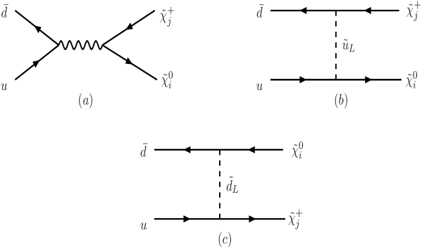
Figure 3: Born diagrams for $u\bar{d}\to\tilde{\chi}^{0}_{i}\tilde{\chi}^{+}_{j}$.

                 

     

         

Figure 5: SPS1a $\hat{s}$-distributions for $\tilde{\chi}^{0}_{1,2}$ production, in association with either $\tilde{g}$ or $\tilde{q}_{L,R}$ or $\tilde{\chi}^{\pm}_{1}$; ($\tilde{\chi}^{c}_{j}\equiv\tilde{\chi}^{\pm}_{j}$).

         

Figure 6: SPS1a $\chi$-distributions for $\tilde{\chi}^{0}_{1,2}$ production, in association with either $\tilde{g}$ or $\tilde{q}_{L,R}$ or $\tilde{\chi}^{\pm}_{1}$; ($\tilde{\chi}^{c}_{j}\equiv\tilde{\chi}^{\pm}_{j}$).

         

         

Figure 7: SPS1aa $\hat{s}$- and $\chi$-distributions for $\tilde{\chi}^{0}_{1,2}$ production in association with either $\tilde{g}$ or $\tilde{\chi}^{\pm}_{1}$.

         

Figure 8: AD(fg9) $\hat{s}$-distributions for $\tilde{\chi}^{0}_{1,2}$ production, in association with either $\tilde{g}$ or $\tilde{q}_{L,R}$ or $\tilde{\chi}^{\pm}_{1}$; ($\tilde{\chi}^{c}_{j}\equiv\tilde{\chi}^{\pm}_{j}$).

         

Figure 9: AD(fg9) $\chi$-distributions for $\tilde{\chi}^{0}_{1,2}$ production, in association with either $\tilde{g}$ or $\tilde{q}_{L,R}$ or $\tilde{\chi}^{\pm}_{1}$; ($\tilde{\chi}^{c}_{j}\equiv\tilde{\chi}^{\pm}_{j}$).

         

         

Figure 10: AD(fg9a) $\hat{s}$- and $\chi$-distributions for $\tilde{\chi}^{0}_{1,2}$ production in association with either $\tilde{g}$ or $\tilde{\chi}^{\pm}_{1}$.

         

Figure 11: SPS1a $\hat{s}$- and $\chi$-distributions in $\tilde{\chi}^{0}_{1}\tilde{\chi}^{0}_{j}$ production for $j=1$ and $j=2$.

         

Figure 12: SPS1aa $\hat{s}$- and $\chi$-distributions in $\tilde{\chi}^{0}_{1}\tilde{\chi}^{0}_{j}$ production for $j=1$ and $j=2$.