Upper limits on sparticle masses from WMAP dark matter constraints with modular invariant soft breaking

An analysis of dark matter within the framework of modular invariant soft breaking is given. In such scenarios inclusion of the radiative electroweak symmetry breaking constraint determines $\tan\beta$ which leads to a more constrained analysis. It is shown that for $\mu$ positive for this constrained system the WMAP data leads to upper limits on sparticle masses that lie within reach of the LHC with also the possibility that some sparticles may be accessible at RUNII of the Tevatron.

1 Introduction

In this talk we will focus on modular invariant soft breaking and an analysis of dark matter within this frameworkcnmodular . We will then show the constraints of WMAPbennett ; spergel , the flavor changing neutral current constraint arising from $b\rightarrow s+\gamma$cleo ; bsgamma ; bsgammanew ; gambino and the constraints of radiative electroweak symmetry breaking (REWSB) put stringent limits on the sparticle masses. Specifically we will show that for the case of $\mu>0$ the WMAP constraints lead to upper limits on sparticle masses which all lie within the reach of the Large Hadron Collider (LHC). Further, it is found that some of these particles may also lie within reach of RUNII of the Tevatron. An analysis of dark matter detection rates is also given and it is shown that for $\mu>0$ the WMAP data leads to direct detection rates which lie within reach of the current and the next generation of dark matter detectorscdms ; genius ; cline ; smith ; cdmsmay2004 ; edelweiss ; damaresult . For the case of $\mu<0$ the detection rates will be accessible to the future dark matter detectors for a part of the allowed parameter space of the models with modular invariant soft breaking and consistent with WMAP and the FCNC constraints. The outline of the rest of the paper is as follows: In Sec.2 we give a brief discussion of modular invariant soft breaking and a determination of $\tan\beta$ with radiative electroweak symmetry breaking constraints. In Sec.3 we give an analysis of the satisfaction of the relic density constraints consistent with WMAP and upper limits on sparticle masses for $\mu>0$. In Sec.4 we discuss the direct detection rates. Conclusions are given in Sec.5.

2 Modular invariant soft breaking

We begin with string theory motivation for considering a modular invariant low energy theory. It is well known that in orbifold string models one has a so called large radius- small radius symmetry

$$R\rightarrow\alpha^{\prime}/R$$ (1)

More generally one has an $SL(2,Z)$ symmetry and such a symmetry is valid even non-perturbatively which makes it very compelling that this symmetry survives in the low energy theory. In formulating an effective low energy theory it is important to simulate as much of the symmetry of the underlying string theory as possible. This provides the motivation for considering low energy effective theories with modular invariancefmtv ; brignole ; nilles ; gaillard .. With this in mind we consider an effective four dimensional theory arising from string theory assumed to have a target space modular $SL(2,Z)$ invariance

$$T_{i}\rightarrow T^{\prime}_{i}=\frac{{a_{i}T_{i}-ib_{i}}}{{ic_{i}T_{i}+d_{i}}},$$

$$\bar{T}_{i}\rightarrow\bar{T}^{\prime}_{i}=\frac{a_{i}\bar{T}_{i}+ib_{i}}{-ic_{i}\bar{T}_{i}+d_{i}},$$

$$(a_{i}d_{i}-b_{i}c_{i})=1,~{}~{}~{}(a_{i},b_{i},c_{i},d_{i}\in Z).$$ (2)

Under the above transformation the superpotential and the Kähler potential transform but the combination

$$G=K+ln(WW^{\dagger})$$ (3)

is invariant. Further, the scalar potential $V$ defined by

$$V=e^{G}((G^{-1})^{i}_{j}G_{i}G^{j}+3)+V_{D}$$

is also invariant under modular transformations. We require that $V_{soft}$ also maintain modular invariance and indeed this invariance will naturally be maintained in our analysis. Typically chiral fields, i.e., quark, leptons and Higgs fields will transform under modular transformations and for book keeping it is useful to assign modular weights to operators. Thus a function $f(T_{i},\bar{T}_{i})$ has modular weights $(n_{1},n_{2})$ if

$$f(T_{i},\bar{T}_{i})\rightarrow(icT_{i}+d)^{n_{1}}(-ic\bar{T}_{i}+d)^{n_{2}}f(T_{i},\bar{T}_{i})$$ (4)

Below we give a list of modular weights for a few cases.

quantity	modular weights $(n_{1},n_{2})$
$|W|$	$(-\frac{1}{2},-\frac{1}{2})$
$e^{i\theta_{W}}$	$(-\frac{1}{2},\frac{1}{2})$
$\eta(T_{i})$	$(\frac{1}{2},0)$
$2\partial_{T_{i}}ln\eta(T_{i})+(T_{i}+\bar{T}_{i})^{-1}$	$(2,0)$
$\partial_{T_{i}}W-(T_{i}+\bar{T}_{i})^{-1}W$	$(1,0)$
$(T_{i}+\bar{T}_{i})$	$(-1,-1)$
$|\gamma_{s}|$	$(0,0)$
$|\gamma_{T_{i}}|$	$(0,0)$
$e^{i\theta_{T_{i}}}$	$(1,-1)$
$e^{i\theta_{S}}$	$(0,0)$
$A^{0}_{\alpha\beta\gamma}$	$(1,0)$
$B^{0}_{\alpha\beta}$	$(1,0)$
$1/\sqrt{f}=1/(\prod(T_{i}+\bar{T}_{i}))^{\frac{1}{2}}$	($\frac{1}{2}$,$\frac{1}{2}$)

Table 1: A list of modular weights under the modular transformations.

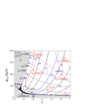
Figure 1: Plot is given of the contours of constant $A_{0},\mu,\tan\beta$ in the $(\gamma_{s}-m_{3/2})$ plane for the case $\mu>0$. The constraint of $b\rightarrow s+\gamma$ decay is shown as a dot-dashed line below which the region is disallowed. The region where the WMAP relic density constraint is satisfied is shown as small shaded area in black. The gray region-I refers to the discarded region with large $\tan\beta$ where Yukawa couplings lie beyond the perturbative domain. The gray region II arises from the absence of REWSB or a $m_{\tilde{\chi}_{1}^{\pm}}$ below the experimental limit. Taken from Ref.cnmodular .

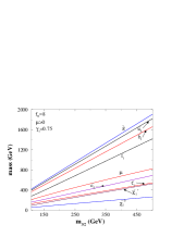
Figure 2: An exhibition of the variation of sparticle masses with $m_{3/2}$ with $\gamma_{s}=0.75$ for the case when $\mu>0$. The WMAP constraint is not exhibited. Taken from Ref.cnmodular

2.1 Modular invariant $V_{soft}$

We begin by considering the condition for the vanishing of the vacuum energy. Using the supergravity form of the scalar potential the condition that vacuum energy vanish is given by

$$|\gamma_{S}|^{2}+\sum_{i=1}^{3}|\gamma_{T_{i}}|^{2}=1$$ (5)

where we have defined $\gamma_{s}$ and $\gamma_{T_{i}}$ as follows

$$\gamma_{s}=(S+\bar{S})G,S/\sqrt{3}=|\gamma_{S}|e^{i\theta_{S}}$$ (6)

$$\gamma_{T_{i}}=(T_{i}+\bar{T}_{i})G,{T_{i}}/\sqrt{3}=|\gamma_{T_{i}}|e^{i\theta_{T_{i}}}$$ (7)

In the investigation of soft breaking we follow the usual procedure of supergravity where one has a visible sector and a hidden sector and supersymmetry breaking occurs in the hidden sector and is communicated to the visible sector by gravitational interactions. For the analysis here we choose the hidden sector to be of the formnathtaylor

$$W_{h}=F(S)/\prod\eta(T_{i})^{2}$$ (8)

and for the Kahler potential we choose

$$K=D(S,\bar{S})-\sum_{i}ln(T_{i}+\bar{T}_{i})+\sum_{i\alpha}(T_{i}+\bar{T}_{i})^{n_{\alpha}^{i}}C_{\alpha}^{\dagger}C_{\alpha}$$ (9)

where $C_{\alpha}$ are the chiral fields. Using the technique of supergravity modelscan the soft breaking potential $V_{soft}$ is given bynathtaylor (for previous analyses see Refs.brignole ; gaillard ; kane

$$V_{soft}=m_{3/2}^{2}\sum_{\alpha}(1+3\sum_{i=1}^{3}n^{i}_{\alpha}|\gamma_{T_{i}}|^{2})c_{\alpha}^{\dagger}c_{\alpha}+(\sum_{\alpha\beta}B^{0}_{\alpha\beta}w^{(2)}_{\alpha\beta}+\sum_{\alpha\beta\gamma}A_{\alpha\beta\gamma}^{0}w_{\alpha\beta\gamma}^{(3)}+H.c.)$$ (10)

where

$$w^{(2)}_{\alpha\beta}=\mu_{\alpha\beta}C_{\alpha}C_{\beta}$$

$$w^{(3)}_{\alpha\beta\gamma}=Y_{\alpha\beta\gamma}C_{\alpha}C_{\beta}C_{\gamma}$$ (11)

The soft breaking parameters $A^{0}$ and $B^{0}$ may be expressed in the form

$$A_{\alpha\beta\gamma}^{0}=-\sqrt{3}m_{3/2}\frac{e^{D/2-i\theta_{W}}}{\sqrt{f}}[|\gamma_{S}|e^{-i\theta_{S}}(1-(S+\bar{S})\partial_{S}lnY_{\alpha\beta\gamma})$$

$$+\sum_{i=1}^{3}|\gamma_{T_{i}}|e^{-i\theta_{T_{i}}}(1+n^{i}_{\alpha}+n^{i}_{\beta}+n^{i}_{\gamma}-(T_{i}+\bar{T}_{i})\partial_{T_{i}}lnY_{\alpha\beta\gamma}-(T_{i}+\bar{T}_{i})n^{i}_{\alpha\beta\gamma}G_{2}(T_{i}))]$$

$$B_{\alpha\beta}^{0}=-m_{3/2}\frac{e^{D/2-i\theta_{W}}}{\sqrt{f}}[1+\sqrt{3}|\gamma_{S}|e^{-i\theta_{S}}(1-(S+\bar{S})\partial_{S}ln\mu_{\alpha\beta})$$

$$+\sqrt{3}\sum_{i=1}^{3}|\gamma_{T_{i}}|e^{-i\theta_{T_{i}}}(1+n^{i}_{\alpha}+n^{i}_{\beta}-(T_{i}+\bar{T}_{i})\partial_{T_{i}}ln\mu_{\alpha\beta}-(T_{i}+\bar{T}_{i})n^{i}_{\alpha\beta}G_{2}(T_{i}))]$$

and further the universal gaugino mass is given by

$$m_{1/2}=\sqrt{3}m_{3/2}|\gamma_{s}|e^{-i\theta_{S}}$$ (12)

2.2 Determination of $\tan\beta$ from modular invariant soft breaking and EWSB constraints

We begin with a discussion of the front factor that appears in $A^{0}$ and $B^{0}$

$$Front~{}factor=e^{D/2-i\theta_{W}}/\sqrt{f}$$ (13)

The front factor has a non vanishing modular weight and the modular invariance of $V_{soft}$ cannot be maintained without it. There are two main elements in this front factor which are of interest to us here. First, there is factor of of $1/\sqrt{f}$ or a factor

$$1/\sqrt{\prod(T_{i}+\bar{T}_{i})}$$ (14)

which produces several solutions to the soft parameters at the self dual points $T_{i}=(1,e^{i\pi/6})$ so that

$$f=8,4\sqrt{3},6,3\sqrt{3}$$ (15)

If we include the complex structure moduli $U_{i}$ then

$$\prod(T_{i}+\bar{T}_{i})\rightarrow\prod(T_{i}+\bar{T}_{i})(U_{i}+\bar{U}_{i})$$

$$f=2^{n}3^{3-\frac{n}{2}}~{}~{}(n=0,..,6)$$ (16)

Assuming that the minimization of the potential occurs at one of these self dual points one finds that there is a multiplicity of soft parameters all consistent with modular invariance. Of course, it may happen that the minimization occurs away from the self dual points. In this case there the f factor will take values outside of the sets given above. The second element that is of interest to us in the front factor is the quantity $e^{D/2}$. This factor is of significance since it can be related to the string gauge coupling constant $g_{string}$ so that

$$e^{-D}=\frac{2}{g_{string}^{2}}$$ (17)

The importance of front factor becomes clear when one considers the electroweak symmetry breaking constraints arising from the minimization of the potential with respect to the Higgs vacuum expectation values $<H_{1}>$ and $<H_{2}>$. In supergravity models one of these relations is used to determine $\mu$ and the other relates the soft parameter $B$ to $\tan\beta$. In supergravity one uses the second relation to eliminate $B$ in favor of $\tan\beta$. However, in the model under consideration $B$ is now determined and thus the second minimization constraint allows one to determine $\tan\beta$ in terms of the other soft parameters and $\alpha_{string}=g_{string}^{2}/4\pi$. Thus specifically the second constraint reads

$$-2\mu B=\sin 2\beta(m_{H_{1}}^{2}+m_{H_{2}}^{2}+2\mu^{2})$$ (18)

Turning this condition around we determine $\tan\beta$ such that

$$\tan\beta=\frac{(\mu^{2}+\frac{1}{2}M_{Z}^{2}+m_{H_{1}}^{2})f_{\alpha}^{1/2}}{\sqrt{2\pi}\mu m_{3/2}\tilde{r}_{B}\alpha_{string}}$$

$$(|-1+3\sum_{i}|\gamma_{i}|^{2}-\sqrt{3}|\gamma_{S}|(1-(S+\bar{S})\partial_{S}ln\mu)|)^{-1}$$ (19)

There is one subtle point involved in the implementation of this equation. One is a relation that holds at the tree level and is accurate only at scales where the one loop correction to this relation is small. This happens when $Q\sim m_{\tilde{t}}$ or $Q\sim$ (highest mass of the spectrum)/2. Thus for the relation of Eq.(19) to be accurate we should use the renormalization group improved values of all the quantities on the right hand side of Eq.(19). This is specifically the case for the Higgs mass parameters and $\mu$. One obtains their values at the high scale $Q$ by running the renormalization group equations between $M_{Z}$ and $Q$. The general analysis used is that of renormalization group analysis of supergravity theories (see, e.g., Ref.an ). Determination of $\tan\beta$ is done in an iterative procedure. One starts with an assumed value of $\tan\beta$ and then one determines $\mu$ through radiative breaking of the electroweak symmetry, one determines the sparticle masses and the Higgs masses and uses these in Eq.(19) to determine the new value of $\tan\beta$. This iteration continues till consistency is obtained. Quite interestingly there are solutions to the iterative procedure, and the convergence is quite rapid. Thus $\tan\beta$ is uniquely determined for each point in the space of other soft parameters provided radiative electroweak symmetry breaking constraints are satisfied. In the analysis the Higgs mixing parameter $\mu$ and specifically its sign plays an important role. Interestingly there is important correlation between the sign of the supersymmetric contribution to the anomalous magnetic moment of the muonyuan and the sign of the $\mu$ parameter. It turns out the current data seems to indicate a positive supersymmetric contribution and a positive $\mu$chattog2 . Thus in the analysis we will mainly focus on $\mu$ positive. However, for the sake of completeness we will also include in our analysis the $\mu<0$ case.

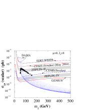
Figure 3: A scatter plot of the spin independent LSP-proton cross section vs LSP mass for the case $\mu>0$ when $\gamma_{s}$ and $m_{3/2}$ are integrated. The region with black circles satisfies the WMAP constraint. Present limits (top three contours) and future accessibility regions are shown. Taken from Ref.cnmodular

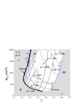
Figure 4: Plot is given of the contours of constant $\tan\beta$ and $\mu$ in the $(\gamma_{s}-m_{3/2})$ plane for the case $\mu<0$. The constraint of $b\rightarrow s+\gamma$ decay is shown as a dot-dashed line below which the region is disallowed. The region where the WMAP relic density constraint is satisfied is shown as small shaded area in black. The gray region I and III are disallowed because of the absence of consistent GUT scale inputs. The region II refers to absence of REWSB or smaller than experimental lower limits of $m_{\tilde{\chi}_{1}^{\pm}}$. The region IV is a no solution zone like I and III, but its location and extent depends on the sensitivity of the minimization scale for REWSB. Region V is the tachyonic $\tilde{\tau}_{1}$ zone. Taken from Ref.cnmodular

3 Analysis of supersymmetric dark matter

There is already a great deal of analysis of supersymmetric dark matter in the literature (For a sample of recent analysesrelated see Refs.ccn2 ; Chattopadhyay:2003yk ; Baer:2003ru ; Binetruy:2003yf ; adkt ; rosz ).. Specifically, over the past year analyses of dark matter matter have focussed on including the constraints of WMAPChattopadhyay:2003xi ; elliswmap ; hb/fp ; Chattopadhyay:2003qh ; gomez Here we discuss the analysis of dark matter within the framework of modular invariant soft breaking where $\tan\beta$ is a determined quantity. Thus using the sparticle spectra generated by the procedure of Sec.2 one can compute the relic density of lightest neutralinos within the modular invariant framework. Quite interesting is the fact that the relic density constraints arising from WMAP data are satisfied by the modular invariant theory in the determined $\tan\beta$ scenario. It is also possible to satisfy the FCNC constraints. One finds that the simultaneous imposition of the WMAP relic density constraints and of the FCNC constraints leads to upper limits on the sparticle masses for the case of $\mu$ postive. The sparticle spectrum that is predicted in this case can be fully tested at the LHC. Further, a part of the parameter space is also accessible at the Tevatron.

We discuss the results now in a quantitative fashion. In Fig.(1) a plot is given of the contours of constant $A_{0}$, constant $\mu$ and constant $\tan\beta$ in the $m_{3/2}-\gamma_{S}$ plane. One finds that there are regions where the relic density constraints consistent with the WMAP data and the FCNC constraints are satisfied. The value of $m_{3/2}$ consistent with all the constraints has an upper limit of about 350 GeV. In Fig.(2) a plot of the sparticle spectrum as a function of $m_{3/2}$ is given for $\gamma_{S}=0.75$. One finds that the sparticle masses with $m_{3/2}<350$ GeV lie in a range accessible at the LHC. In fact, for a range of the parameter space some of the sparticles may also be accessible at the Tevatron. Thus much of the Hyperbolic Branch/Focus Point (HB/FP) regionChan:1997bi seems to be eliminated by the constraints of WMAP and FCNC within the modular invariant soft breakingcnmodular .

In Fig.(3) an analysis of the direct detection cross-section for $\sigma_{\chi-p}$ as a function of the LSP mass is given. One finds that all of the parameter space of the model will be probed in the current and future dark matter colliders. An analysis analogous to that of Fig.(1) but for $\mu<0$ is given in Fig.(4) while an analysis analogous to Fig.(3) is given in Fig.(5). In this case one finds that a part of the parameter space consistent with WMAP can be probed in the current and future dark matter experiments. Finally, the analysis presented above is done under the assumption that the chiral fields have zero modular weights. For non-vanishing modular weights one needs a realistic string model and an analysis of the sparticle spectra and dark matter for such a model should be worthwhile using the above framework.

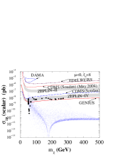
Figure 5: A scatter plot of the spin-dependent LSP-proton cross section vs LSP mass for the case when $\mu<0$. The region with black circles satisfies the WMAP constraint. Taken from Ref.cnmodular .

4 Conclusion

In this paper we have analyzed the implications of modular invariant soft breaking in a generic heterotic string scenario under the constraint of radiative breaking of the electroweak symmetry. It was shown that in models of this type $\tan\beta$ is no longer an arbitrary parameter but a determined quantity. Thus the constraints of modular invariance along with a determined $\tan\beta$ reduced the allowed parameter space of the model. Quite remarkably one finds that the reduced parameter space allows for the satisfaction of the accurate relic density constraints given by WMAP. Further, our analysis shows that the WMAP constraint combined with the FCNC constraint puts upper limits on the sparticle masses for the case $\mu>0$ which are remarkably low implying that essentially all of the sparticles would be accessible at the LHC and some of the sparticles may also be visible at the Tevatron. Further, we analysed the direct detection rates in dark matter detectors in such a scenario. It is found that for the case $\mu>0$ the dark matter detection rates fall within the sensitivities of the current and future dark matter detectors. For the case $\mu<0$ a part of the allowed parameter space will be accessible to dark matter detectors. It should be of interest to analyze scenarios of the type discussed above with determined $\tan\beta$ in the investigation of other SUSY phenomena. Further, it would be interesting to examine if similar limits arise in models with modular invariance in extended MSSM seenarios, such as the recently proposed Stueckelberg extension of MSSMkn2 .

Acknowledgements
This work is supported in part by NSF grant PHY-0139967.

References

- (1) U. Chattopadhyay and P. Nath, arXiv:hep-ph/0405157.(to appear in Phys. Rev. D)
- (2) C. L. Bennett et al., Astrophys. J. Suppl. 148, 1 (2003), [arXiv:astro-ph/0302207].
- (3) D. N. Spergel et al., Astrophys. J. Suppl. 148, 175 (2003), [arXiv:astro-ph/0302209].
- (4) K. Abe et al. [Belle Collaboration], Phys. Lett. B 511, 151 (2001) [arXiv:hep-ex/0103042]; S. Chen et.al. (CLEO Collaboration), Phys. Rev. Lett. 87, 251807 (2001); R. Barate et al. [ALEPH Collaboration], Phys. Lett. B 429, 169 (1998).
- (5) P. Nath and R. Arnowitt, Phys. Lett. B 336, 395 (1994) [arXiv:hep-ph/9406389] ; Phys. Rev. Lett. 74, 4592 (1995) [arXiv:hep-ph/9409301] ; F. Borzumati, M. Drees and M. Nojiri, Phys. Rev. D 51, 341 (1995); H. Baer, M. Brhlik, D. Castano and X. Tata, Phys. Rev. D 58, 015007 (1998).
- (6) H. Baer, A. Belyaev, T. Krupovnickas and A. Mustafayev, arXiv:hep-ph/0403214; K. i. Okumura and L. Roszkowski, Journal of High Energy Physics, 0310, 024 (2003) [arXiv:hep-ph/0308102]; M. Carena, D. Garcia, U. Nierste, C.E.M. Wagner, Phys. Lett. B499 141 (2001); G. Degrassi, P. Gambino, G.F. Giudice, JHEP 0012, 009 (2000); M. Ciuchini, G. Degrassi, P. Gambino and G. F. Giudice, Nucl. Phys. B 534, 3 (1998).
- (7) P. Gambino and M. Misiak, Nucl. Phys. B611, 338 (2001); P. Gambino and U. Haisch, JHEP 0110, 020 (2001); A.L. Kagan and M. Neubert, Eur. Phys. J. C7, 5(1999). A.L. Kagan and M. Neubert, Eur. Phys. J. C27, 5(1999).
- (8) R. Abusaidi et.al., Phys. Rev. Lett.84, 5699(2000), ”Exclusion Limits on WIMP-Nucleon Cross-Section from the Cryogenic Dark Matter Search”, CDMS Collaboration preprint CWRU-P5-00/UCSB-HEP-00-01 and astro-ph/0002471.
- (9) H.V. Klapdor-Kleingrothaus, et.al., ”GENIUS, A Supersensitive Germanium Detector System for Rare Events: Proposal”, MPI-H-V26-1999, hep-ph/9910205; H. V. Klapdor-Kleingrothaus, “Search for dark matter by GENIUS-TF and GENIUS,” Nucl. Phys. Proc. Suppl. 110, 58 (2002) [arXiv:hep-ph/0206250].
- (10) D. Cline, “Status of the search for supersymmetric dark matter,” arXiv:astro-ph/0306124.
- (11) D. R. Smith and N. Weiner, Nucl. Phys. Proc. Suppl. 124, 197 (2003) [arXiv:astro-ph/0208403].
- (12) [CDMS Collaboration], “First Results from the Cryogenic Dark Matter Search in the Soudan Underground Lab,” arXiv:astro-ph/0405033.
- (13) G. Chardin et al. [EDELWEISS Collaboration], Nucl. Instrum. Meth. A 520, 101 (2004); A. Benoit et al., Phys. Lett. B545, 43 (2002), [arXiv:astro-ph/0206271].
- (14) R. Bernabei et al. [DAMA Collaboration], Phys. Lett. B 480, 23 (2000).
- (15) S. Ferrara, N. Magnoli, T. R. Taylor and G. Veneziano, Phys. Lett. B 245, 409(1990); A. Font, L. E. Ibanez, D. Lüst and F. Quevedo, Phys. Lett. B 245, 401(1990); H. P. Nilles and M. Olechowski, Phys. Lett. B 248, 268(1990); P. Binetruy and M. K. Gaillard, Phys. Lett. B 253, 119(1991); M. Cvetic, A. Font, L. E. Ibanez, D. Lüst and F. Quevedo, Nucl. Phys. B 361, 194(1991).
- (16) A. Brignole, L. E. Ibanez, C. Munoz and C. Scheich, Z. Phys. C 74, 157 (1997); B. de Carlos, J. A. Casas and C. Munoz, Nucl. Phys. B 399, 623(1993); A. Brignole, L. E. Ibanez and C. Munoz, Phys. Lett. B 387,769(1996).
- (17) H. P. Nilles, Phys. Lett. B 115, 193(1982); S. Ferrara, L. Girardello and H. P. Nilles, Phys. Lett. B 125, 457(1983); M. Dine, R. Rohm, N. Seiberg and E. Witten, Phys. Lett. B 156, 55(1985); C. Kounnas and M. Porrati, Phys. Lett. B 191, 91(1987).
- (18) P. Binetruy, M. K. Gaillard and B. D. Nelson, Nucl. Phys. B 604, 32(2001); M. K. Gaillard, B. D. Nelson and Y. Y. Wu, Phys. Lett. B 459, 549(1999); M. K. Gaillard and J. Giedt, Nucl. Phys. B 636, 365(2002).
- (19) P. Nath and T. R. Taylor, Phys. Lett. B 548, 77 (2002) [arXiv:hep-ph/0209282].
- (20) A. H. Chamseddine, R. Arnowitt and P. Nath, Phys. Rev. Lett. 49, 970 (1982) ; R. Barbieri, S. Ferrara and C. A. Savoy, Phys. Lett. B 119, 343(1982) ; P. Nath, R. Arnowitt and A. H. Chamseddine, Nucl. Phys. B 227, 121 (1983) ; L. Hall, J. Lykken, and S. Weinberg, Phys. Rev. D 27, 2359 (1983); P. Nath, “Twenty years of SUGRA,” arXiv:hep-ph/0307123.
- (21) G. L. Kane, J. Lykken, S. Mrenna, B. D. Nelson, L. T. Wang and T. T. Wang, Phys. Rev. D 67, 045008 (2003) [arXiv:hep-ph/0209061]; B. C. Allanach, S. F. King and D. A. J. Rayner, arXiv:hep-ph/0403255; P. Binetruy, A. Birkedal-Hansen, Y. Mambrini and B. D. Nelson, arXiv:hep-ph/0308047 ; A. Birkedal-Hansen and B. D. Nelson, Phys. Rev. D 64, 015008 (2001) [arXiv:hep-ph/0102075].
- (22) B. Kors and P. Nath, Nucl. Phys. B 681, 77 (2004) [arXiv:hep-th/0309167].
- (23) R. Arnowitt and P. Nath, Phys. Rev. Lett. 69, 725 (1992).
- (24) T. C. Yuan, R. Arnowitt, A. H. Chamseddine and P. Nath, Z. Phys. C 26, 407 (1984) ; D.A. Kosower, L.M. Krauss, N. Sakai, Phys. Lett. B 133, 305 (1983); J.L. Lopez, D.V. Nanopoulos, X. Wang, Phys. Rev. D 49, 366 (1994); U. Chattopadhyay and P. Nath, Phys. Rev. D 53, 1648 (1996) [arXiv:hep-ph/9507386]. ; T. Moroi, Phys. Rev. D 53, 6565 (1996); T. Ibrahim and P. Nath, Phys. Rev. D 61, 095008 (2000) [arXiv:hep-ph/9907555]. ; Phys. Rev. D 58, 111301 (1998) [arXiv:hep-ph/9807501]. ; Phys. Rev. D62, 015004(2000); U.Chattopadhyay , D. K. Ghosh and S. Roy, Phys. Rev. D 62, 115001 (2000).
- (25) U. Chattopadhyay and P. Nath, Phys. Rev. Lett. 86, 5854 (2001). For a more complete list of references see, U. Chattopadhyay, A. Corsetti and P. Nath, arXiv:hep-ph/0202275.
- (26) See also talks by Howard Baer, Wim de Boer, Bhasker Dutta, Paolo Gondolo, Keith Olive, Leszek Roszkowski, and Ioannis Vergados in these proceedings.
- (27) U. Chattopadhyay, A. Corsetti and P. Nath, Phys. Rev. D 66, 035003 (2002) [arXiv:hep-ph/0201001]; M. E. Gomez, G. Lazarides and C. Pallis, Phys. Rev. D 61, 123512 (2000) [arXiv:hep-ph/9907261] ; M. E. Gomez, G. Lazarides and C. Pallis, Phys. Lett. B 487, 313 (2000) [arXiv:hep-ph/0004028].
- (28) U. Chattopadhyay and D. P. Roy, Phys. Rev. D 68, 033010 (2003) [arXiv:hep-ph/0304108].
- (29) H. Baer, A. Belyaev, T. Krupovnickas and X. Tata, JHEP 0402, 007 (2004) [arXiv:hep-ph/0311351].
- (30) P. Binetruy, Y. Mambrini and E. Nezri, arXiv:hep-ph/0312155.
- (31) R. Arnowitt, B. Dutta, T. Kamon and M. Tanaka, Phys. Lett. B 538, 121 (2002) [arXiv:hep-ph/0203069].
- (32) Y. G. Kim, T. Nihei, L. Roszkowski and R. Ruiz de Austri, JHEP 0212, 034 (2002) [arXiv:hep-ph/0208069].
- (33) U. Chattopadhyay, A. Corsetti and P. Nath, Phys. Rev. D 68, 035005 (2003) [arXiv:hep-ph/0303201].
- (34) J. Ellis, K. A. Olive, Y. Santoso and V. C. Spanos, Phys. Lett. B565, 176, (2003), [arXiv:hep-ph/0303043]; H. Baer and C. Balazs, JCAP 0305, 006 (2003), [arXiv:hep-ph/0303114]; A. B. Lahanas and D. V. Nanopoulos, Phys. Lett. B568, 55, (2003) [arXiv:hep-ph/0303130].
- (35) H. Baer, C. Balazs, A. Belyaev and J. O’Farrill, JCAP 0309, 007 (2003), [arXiv:hep-ph/0305191]; H. Baer, C. Balazs, A. Belyaev, T. Krupovnickas and X. Tata, JHEP 0306, 054 (2003) [arXiv:hep-ph/0304303]; R. Arnowitt, B. Dutta and B. Hu, arXiv:hep-ph/0310103; J. R. Ellis, K. A. Olive, Y. Santoso and V. C. Spanos, Phys. Lett. B 573, 162 (2003) [arXiv:hep-ph/0305212]; J.D. Vergados, P. Quentin and D. Strottman, hep-ph/0310365.
- (36) For a review see, U. Chattopadhyay, A. Corsetti and P. Nath, Phys. Atom. Nucl. 67, 1188 (2004) [Yad. Fiz. 67, 1210 (2004)] [arXiv:hep-ph/0310228]. ; A. B. Lahanas, N. E. Mavromatos and D. V. Nanopoulos, Int. J. Mod. Phys. D 12, 1529 (2003) [arXiv:hep-ph/0308251].
- (37) M. E. Gomez, T. Ibrahim, P. Nath and S. Skadhauge, Phys. Rev. D 70, 035014 (2004) [arXiv:hep-ph/0404025]. ; T. Nihei and M. Sasagawa, arXiv:hep-ph/0404100; M. Argyrou, A. B. Lahanas, D. V. Nanopoulos and V. C. Spanos, arXiv:hep-ph/0404286. ; M. E. Gomez, T. Ibrahim, P. Nath and S. Skadhauge, arXiv:hep-ph/0410007.
- (38) K. L. Chan, U. Chattopadhyay and P. Nath, Phys. Rev. D 58, 096004 (1998) [arXiv:hep-ph/9710473] ;. J. L. Feng, K. T. Matchev and T. Moroi, Phys. Rev. D 61, 075005 (2000).
- (39) B. Kors and P. Nath, arXiv:hep-ph/0406167. ; Phys. Lett. B 586, 366 (2004) [arXiv:hep-ph/0402047].