Solar neutrinos and 1-3 leptonic mixing
Srubabati Goswami1,
Alexei Yu. Smirnov2,3,
1Harish-Chandra Research Institute, Chhatnag Road, Jhusi, Allahabad 211 019, India,
2The Abdus Salam International Centre for Theoretical
Physics,
I-34100, Trieste, Italy
3Institute for Nuclear Research, Russian Academy of
Scienses, Moscow, Russia
Abstract
Effects of the 1-3 leptonic mixing on the solar neutrino observables are studied and the signatures of non-zero are identified. For this we have re-derived the formula for -survival probability including all relevant corrections and constructed the iso-contours of observables in the plane. Analysis of the solar neutrino data gives ( C.L.) for eV2. The combination of the ratio CC/NC at SNO and gallium production rate selects (). The global fit of all oscillation data leads to zero best value of . The sensitivity ( error) of future solar neutrino studies to can be improved down to 0.01 - 0.02 by precise measurements of the pp-neutrino flux and the CC/NC ratio as well as spectrum distortion at high ( MeV) energies. Combination of experimental results sensitive to the low and high energy parts of the solar neutrino spectrum resolves the degeneracy of angles and . Comparison of as well as measured in the solar neutrinos and in the reactor/accelerator experiments may reveal new effects which can not be seen otherwise.
1 Introduction
Determination of the 1-3 mixing parameterized by the angle is of great importance for phenomenology, for future experimental programs, and eventually, for understanding the underlying physics.
At present, for we only have the upper bounds. The CHOOZ [1] reactor experiment (see also PaloVerde [2]) gives
| (1) |
for eV2. The recent global fit of the oscillation results which includes also the solar salt phase II SNO, KamLAND and atmospheric neutrino data leads to [3]
| (2) |
According to [4] the 90% C.L. bound is . The limit (2) is slightly better than the earlier (before SNO salt phase II) limits [5, 6, 7] . In [8] even stronger upper bound is quoted: .
The combined fit of the CHOOZ, K2K and atmospheric neutrino results (without solar ones) gives [3]
| (3) |
(See also [9].)
Comparison of the bounds (2) and (3)
shows that effect of inclusion of the solar neutrino data in the global
fit is weak but not negligible: the bounds improve by .
Future long baseline experiments are geared towards precision measurement of . MINOS [10] and CERN to Gran-Sasso [11] alone will be able to only slightly improve the limit (2) down to
| (4) |
J-PARC accelerator experiment [12] will have substantially higher sensitivity:
| (5) |
but when all correlations and degeneracies of parameters are taken into account the estimated sensitivity reduces to [13].
The Double-CHOOZ reactor experiment [14] will be able to improve the bound down to
| (6) |
for eV2. It provides a clean channel of measurement of complementary to accelerator measurements [15],[13].
Detection of neutrinos from the Galactic supernova can, in principle, probe down to . The problem here is large uncertainties in the original neutrino fluxes. Essentially one can find whether is larger or smaller than . Both the upper and the lower bounds on may be established if is in the range [16, 17].
Ultimate sensitivity, ,
can be achieved at the neutrino factories [18].
Influence of the 1-3 mixing on the detected solar neutrino fluxes has been considered in a number of publications before [19] - [34], [7]. The present solar neutrino data are not precise enough to really probe in the allowed range (2,3), but on the other hand the bounds obtained using the solar data only are not much weaker than those from the reactor and atmospheric neutrino results. Indeed, recent analysis of the solar neutrino data alone [3] gives
| (7) |
and very weak bound. Inclusion of the latest KamLAND data improves the latter bound substantially [3]
| (8) |
(This can be compared with (3).)
The 1-3 mixing taken at the present upper bound modifies the allowed region of the parameters obtained from the global fit. It shifts the region toward larger and smaller , however the shift of the best fit point is within [7].
It was noticed that the Earth matter regeneration effect has
strong dependence on , as [35].
This can be used to determine in future solar neutrino
experiments [35, 36].
Measurements of the pp-neutrino fluxes will also improve the
sensitivity to [21].
In this paper we study in details possible effects of 1-3 mixing on the solar neutrino observables. We analyze the present determination of and and evaluate the sensitivity of future solar neutrino experiments to .
The paper is organized as follows. We first (sec. 2) re-derive the survival probability including all relevant corrections and estimating accuracy of the approximations. We consider dependence of the probability on . In sec. 3 we find simple analytic expressions for the probability in the high and low energy limits. In sec. 4 we introduce the plots and derive the equations for contours of constant values of observables in this plot. In sec. 5 we find the allowed region of parameters and and consider the bounds on these parameters from individual measurements. In sec. 6 the sensitivity of future, in particular, the low energy (LowNu) solar neutrino experiments to 1-3 mixing, is estimated. We discuss possible implications of future measurements of in sec 7. Our results are summarized in sec. 8.
2 The survival probability and
The analytic formula which describes conversion of the solar neutrinos in the case of three neutrino mixing and mass split hierarchy, , has been derived long time ago [31, 32]. Here and are the mass splits associated to 1-3 mixing and to the main channel of the solar neutrino conversion correspondingly. The formula was analyzed and further corrected recently [33, 34, 35].
In view of future precision measurements
one needs to have an accurate formula for the probability
with all relevant corrections included and
errors due to approximation made estimated.
For this reason we re-derive the formula
in a simple and adequate way which employs features of the
Large Mixing Angle (LMA) MSW solution.
We will use a very high level of
adiabaticity [37, 38, 39, 40] in whole
system.
Due to loss of coherence between the mass eigenstates, (i = 1, 2, 3), the survival probability can be written as
| (9) |
where is the probability of conversion in the Sun and is the oscillation probability inside the Earth. Strong adiabaticity of the neutrino conversion in the Sun leads immediately to
| (10) |
where is the -element of neutrino mixing matrix in matter in the production point. Indeed, determines the admixture of the eigenstate, , in the neutrino state in the initial point. Then due to adiabaticity transforms to when neutrino propagates to the surface of the Sun. Corrections due to the adiabaticity violation are negligible [40]: , where is the adiabaticity parameter. For MeV we find .
Combining (9) and (10) we obtain
| (11) |
In the absence of the Earth matter effect (the day signal) we have
| (12) |
where are the elements of the vacuum mixing matrix.
In what follows we will neglect the Earth matter effect on the 1-3 mixing which is determined by , (here is the typical potential inside the Earth). Therefore
| (13) |
The Earth matter effect on two other probabilities can be described by the term defined as the deviation of probability from the no-oscillation one:
| (14) |
Then the unitarity condition, and (13) lead to
| (15) |
Plugging (12, 13, 15) into (11) we obtain
| (16) |
We will use the standard parameterization of the mixing matrix in terms of mixing angles:
| (17) |
and similar definition holds for the matrix elements in matter with substitution and . The angle is identified with the “solar mixing angle”.
In terms of mixing angles the probability (16) can be rewritten as
| (18) |
where is the usual two neutrino adiabatic probability:
| (19) |
For the probability (18) coincides with the one obtained
in [32].
Let us find the mixing angle in matter. The Hamiltonian of 3 system can be written in the flavor basis as
| (20) |
Here , , and , where is the matter density and is the electron number density fraction.
Performing rotations we arrive at the basis in which the Hamiltonian becomes
| (21) |
If the matter effect is small we can neglect mixing of the third state (off-diagonal terms of the matrix ). This state then decouples and for the rest of the system the Hamiltonian becomes
| (22) |
where .
In the lowest approximation the matter effect on the 1-3 mixing can be found making an additional 1-3 rotation which eliminates the 1-3 elements in (21). The angle of rotation, , is given by
| (23) |
where
| (24) |
So, approximately, .
The additional 1-3 rotation generates negligible 2-3 elements 111Elimination of this term requires an additional 2-3 rotation by the angle .
| (25) |
It also leads to corrections to the 1-2 block of the Hamiltonian:
| (26) |
In the first order in the rotation decouples the third state. So, the 1-3 mixing angle in matter is given by
| (27) |
and using (23) we obtain
| (28) |
(See also [33].) For typical energy MeV the relative matter correction is (10 - 15)%. The correction is negligible at low energies.
The 1-2 mixing in matter is determined from diagonalization of
(22) or (26). Neglecting very small correction
() in (26)
one obtains for the standard
formula with substitution
.
Let us find dependence of on the 1-3 mixing explicitly. The probability of conversion can be written in terms of the amplitudes of transitions between the mass states , , as
| (29) |
Since in the absence of matter effect and , in the lowest approximation in , we obtain
| (30) |
The transition amplitude should be found by solving the evolution equation with the Hamiltonian (26). It is proportional to the potential: , and consequently, (30) can be rewritten as
| (31) |
where
| (32) |
is the regeneration factor given by the amplitude , and it does not depend on .
The regeneration factor integrated with the exposure function over the zenith angle can be estimated as
| (33) |
where is the potential at the surface of the Earth. Indeed, the integrated effect is mainly due to the oscillations in the mantle of the Earth along the trajectories which are not too close to the horizontal ones. (For the core crossing trajectories the effect of the core is attenuated [41].) In turn, for the mantle trajectories the adiabaticity is nearly fulfilled [40] and therefore characteristics of oscillations (averaged probability and depth of oscillations) are determined by the potentials in the initial and final points of the trajectory, that is, by the potential near the surface of the Earth (for numerical consideration see [42]).
Inserting the expression for into (18) we obtain
| (34) |
Taking the mixing angle in the first order in we find
| (35) |
Notice that the pre-factor
which describes the matter effect on
the 1-3 mixing differs in the high and low energy limits.
The expression (34) can be rewritten as
| (36) |
where
is the total survival probability for
mixing which includes both the conversion in the Sun and
the oscillations in the Earth.
depends on via the effective matter potential
.
The probability should be averaged over the distribution of the neutrino sources in the Sun. For the -component of the solar neutrino spectrum () the averaged probability can be written as [40]
| (37) |
where is the effective value of the matter potential
in the region of production of the neutrino component.
is an additional correction due to the
integration over the production region [40],
and in what follows we will neglect it.
Notice there are three features of dynamics of propagation which allow one to immediately derive the survival probability in terms of the probabilities:
1). Adiabaticity of propagation of the third neutrino;
2). Negligible Earth matter effect on 1-3 mixing;
3). Averaging of oscillations and loss of coherence of the third mass eigenstate.
Essentially this means
that the third neutrino eigenstate decouples from dynamics and
propagates independently. Its contribution to the probability adds
incoherently.
Therefore the problem is reduced to two neutrino
problem and additional factors in (34)
are just projection of the flavor
basis onto the basis of states which
contains the decoupling state .
In (36) factors and
are from the projection in the initial state,
whereas the factors and
are from projection in the final state.
Up to negligible corrections the expression for the probability (36) can be rewritten in form
| (38) |
where
| (39) |
which coincides with the form without matter corrections to 222Strictly, this is correct in the high energy or low energy limits, where depends very weakly on the potential. At low energies the matter corrections are negligible anyway (see eq. (24).. This means that the matter effect on the 1-3 mixing in the probability can be accounted by renormalization of . Inversely, using usual formula for the probability without matter corrections in the analysis of the data we determine averaged over the relevant energy interval. Then the true vacuum mixing angle will be smaller:
| (40) |
Here is the value averaged over the relevant energy range. Renormalization depends on the neutrino energy: at high energies and in the -neutrino range, and the latter can be neglected.
3 Two limits
As we will see, the expected sensitivity of solar neutrino studies to the 1-3 mixing will not be better than . According to (36) that would correspond to the change of the survival probability
| (41) |
Therefore in the present discussions we can neglect various corrections to the probability which are much smaller that 0.01. In particular,
-
•
the term can be neglected in eq. (36);
-
•
the matter effect on the 1-3 mixing is small and can be taken into account as a small renormalization of (see sec. 2);
-
•
we will neglect corrections in .
In qualitative consideration we will use simplified expressions for the survival probability obtained in the limits of high and low energies. In fact, all relevant fluxes are either in the low (pp, Be, N, O, pep) or in the high, MeV (B, hep), energy limits. The expansion parameter equals
| (42) |
at high energies and at
low energies 333Notice that in [40] we use
different definition of : ..
1). In the high energy limit, performing expansion of (37) in we find the survival probability
| (43) |
Here the first term is due to the non-oscillatory adiabatic conversion. In the second term, which describes the effect of averaged oscillations, dependence on is absent. In contrast, the third (regeneration) term has the strongest dependence on [35]. It originates from the common factor and the effective potential in the case which contains another factor.
In the lowest order in we can rewrite (43) as
| (44) |
Neglecting the oscillation corrections (second term) and the double suppressed term we obtain
| (45) |
2). For the low energy neutrinos ( MeV), the matter effect is small and in the lowest order in we have
| (46) |
Here the first term is the effect of averaged vacuum oscillations. The second one gives the matter effect correction which contains strong dependence on . An additional second power of originates from the matter potential. The regeneration effect is neglected. Numerical calculations confirm that the linear in approximation (46) works well up to MeV.
In the lowest order in we find from (46)
| (47) | |||
| (48) |
For very low energies (pp-neutrino range) the matter corrections can be neglected, so that
| (49) |
-
•
The dependences of the probability on for the high energies and low energies are opposite: increases whereas decreases with decrease of .
-
•
In contrast, and both decrease with increase of . So, and correlate at low energies and anti-correlate at high energies. For the neutrinos an increase of can be compensated by increase of , whereas at low energies (for the neutrinos), should decrease to compensate increase of .
-
•
Both for the high and low neutrino energies the dependence of probability on appears via small corrections only, and therefore, is weak.
Apparently strong dependence on cancels in the ratio of probabilities (or the ratio of the corresponding observables):
| (50) |
Notice that dependence of the ratio on appears via small corrections and it can be neglected in the first approximation. So, measurements of the ratio gives . Then one of the probabilities (in low or high limits) can be used to find .
4 plots and iso-contours of observables
There are two important features of the problem:
-
•
Weak dependence of the probability and observables on within the allowed region;
-
•
degeneracy.
Let us consider these features in some details.
1). The KamLAND spectral data has shown high precision in determination of . The relative error
| (51) |
is about (3) at the present, and with 3 kTy statistics from KamLAND this can further reduce down to 7% [43].
As follows from (43) and (48), variation of the probability in the high energy limit with equals
| (52) |
For MeV and
,
we find .
In the low energy part, variations of the probability with are even weaker:
| (53) |
For MeV we find
.
2). According to the discussion in sec. 2,
in the first approximation, all
experiments which probe the high energy part of the spectrum
are sensitive to the same combination of
mixing angles and . Similar
statement is true for the low energy experiments
but the combination of mixing angles is different.
Therefore to determine and separately
one needs to employ both types of
experiments.
In view of these two features, we will present results of
our study in plane
for fixed values of .
Let us construct the contours of constant values of various observables in the plane. Essentially, the iso-contours for a given observable coincide with the contours of constant survival probability averaged over the relevant energy range with the corresponding cross-section:
| (54) |
The survival probabilities found in the high and low energy limits determine two different types of the iso-contours. For the high energy observables ( MeV), using Eq. (44), we find an analytic expression for the contours of constant :
| (55) |
where
| (56) |
is the averaged over the neutrino energy value of folded with the cross-section, energy resolution of detector, etc.. In the allowed range of (with the average value of mixing denoted by ) the strongest dependence comes from the denominator of (55):
| (57) |
So, in the first approximation the contours are straight lines.
This reproduces well the results of numerical
calculations presented in sec. 5, 6. Notice that
increases with .
For the low energy observables, , using (48), we obtain expressions for the iso-contours as
| (58) |
where
| (59) |
In the rough approximation
| (60) |
and it has minimum at . Other terms in (58) shift this minimum to smaller values of . So, in the region of interest, , the lines of constant values of observables have negative slope: decreases with .
5 Constraints on the mixing parameters from the present experiments
In this section we describe the results of our numerical computations.
We first perform the global analysis of different data samples. Some details of the analysis follow. The CHOOZ depends on and in our fit we vary this parameter freely in the range allowed by the zenith angle SuperKamiokande atmospheric neutrino data [44]. The details of procedure for the solar and CHOOZ data can be found in [28] while the KamLAND analysis follows the method outlined in [29, 6]. We use the KamLAND data from the latest version of paper [45] where new source of the background has been taken into account.
For the solar neutrinos we include the data on total rates from the radiochemical experiments Cl [46] and Ga (SAGE, GALLEX and GNO combined) [47], the Superkamiokande day-night spectrum data [48], the SNO CC (charged current), ES (neutrino-electron scattering) and NC (neutral current) rates from the salt phase-I, the combined CC+ES+NC energy spectrum from the pure D2O phase [49] as well as the day-night spectrum data of CC,ES and NC events from the salt-phase II [50].
The neutrino flux normalization, , where is the true flux and is the flux predicted in the SSM [51], is left as a free parameter in the fit. Essentially is fixed by the NC data from the SNO experiment. For the other fluxes and their uncertainties we use the predictions from the Standard Solar Model (SSM) [51].
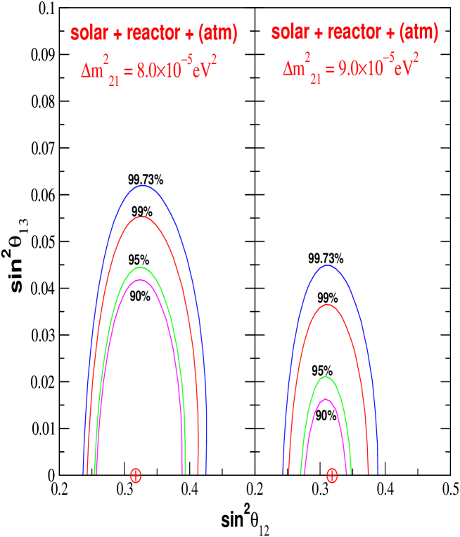
In fig. 1 we show the allowed regions of the parameters (for two different values of ) which follow from the global fit of all available solar neutrino data as well as data from reactor experiments KamLAND and CHOOZ. The contours are marginalised over . The global minimum has been obtained by letting all the parameters (including ) vary freely in the fit. With this, the values of parameters in the global minimum come at
| (61) |
The two panels in fig. 1
correspond to two fixed illustrative values of
from the current allowed range.
The contours are plotted with respect to the global minimum
(61) using the
definition of which corresponds to 3 parameters.
The upper bound, (99% C.L.)
is tighter than the one obtained without including the phase-II
SNO salt data (0.061).
According to fig. 1 with increase of
the allowed region shifts to smaller ;
with increase of
the value of in minimum of practically does
not change.
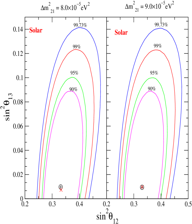
We have performed the global fit of the solar neutrino data only. The best-fit values of parameters are found to be
| (62) |
Now the 1-3 mixing is non-zero but statistically insignificant. The solar is somewhat flat in the region . For and 0.02 we obtain the = 113.84 and 114.04 correspondingly.
Notice that we find small boron neutrino flux: in the units of flux predicted in [51]. Recent calculations of fluxes with new radiative opacities and the heavy element abundances give even smaller value [52].
In fig. 2 we show the constant contours obtained from global analysis of the solar neutrino data only and when is fixed. The contours have been calculated with respect to the global minimum (62) and using the values corresponding to 3 parameters. We also show the local minima found for fixed values of . In particular, for eV2 we obtain
| (63) |
The best fit value of changes with very
weakly, e.g., for eV2 we find
.
The fig. 2 shows also that at present
the solar data alone has a weak sensitivity to :
the 90% C.L. bound equals .
Inversely, the values of allowed by the
global fit (2) have weak impact on the global analysis of the
solar neutrino data. From fig. 2 we find that
with increase of from
0 to 0.05 the best fit value and allowed region of
shift to larger values by
only which is smaller than
error and in agreement with earlier estimations in
[22].
Let us now consider bounds on mixing angles and from individual observables.
1). At present only the gallium experiments can be considered as the low energy experiments. For the Ge-production rate, , we have
| (64) |
where is the contribution to the rate from the th component of the solar neutrino flux according to the SSM, is the corresponding effective (averaged over the energy range) survival probability. The rate has the contributions both from the low and high energy parts of the spectrum, though the latter (from boron neutrinos) is much smaller. We can subtract the boron neutrino effect, , using experimental results from SNO: . Taking the flux from SNO as an input, we find that the neutrino contribution equals SNU and then SNU for the rest of the neutrinos [47].
The conversion effect on is described by the probability in low energy limit:
| (65) |
where
| (66) |
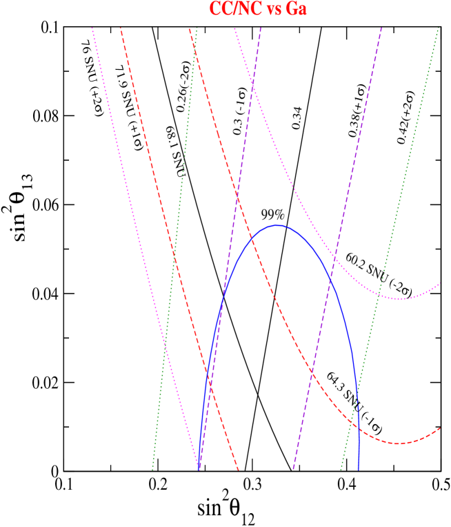
At the same time we find that dependence of the total rate on and the high energy conversion effect is very weak: variations of would produce change of about 0.4 SNU. Therefore results of numerical calculations are given in figs. 3, 4, 5, for and . We show the contours of constant total rate which correspond to the present central value as well as to and deviations from it. The contours are well described by the analytical expression given in (58) with and .
For zero 1-3 mixing the central value SNU
corresponds to ,
and the best fit value
is accepted at level.
For a given , increases
with decrease of .
Taking the best fit value (see
eq. (62))
and SNU we find .
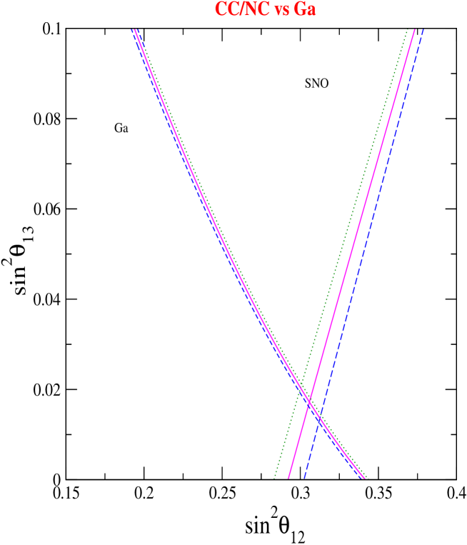
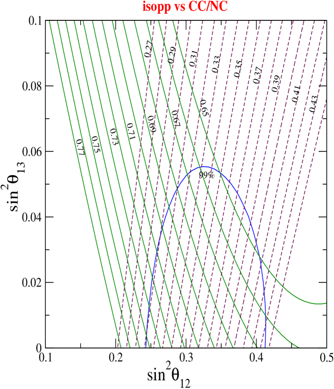
2). The CC/NC ratio of events at SNO is given by the integrated (with cross-section) survival probability at high energies: CC/NC . The iso-contours are described approximately by Eq. (55) with CC/NC. The results of exact numerical calculations are shown in fig. 3. The iso-contours are constructed for the present central value of CC/NC as well as for its and deviations. At the central value of CC/NC gives .
As seen from fig. 3, the combination of SNO CC/NC and Ga-results prefers the non-zero but statistically insignificant 1-3 mixing. The iso-contours of the central observed values of CC/NC and cross at
| (67) |
which is about deviation from zero. Here is evaluated from the fig. 3 using CC/NC and measurements.
The CC/NC ratio is free of the 8B neutrino normalization
factor . Iso-contours for the
Ge-production rate are constructed for =1, i.e.,
for the SSM value of the 8B flux.
The dependence of on essentially disappears if one uses
for the boron neutrino flux the value measured by NC in SNO or
by SK. In any case the influence of uncertainty related to
on the intersection of iso-contours is weak.
Larger uncertainty ( SNU) follows from the Be-neutrino flux
contribution. That leads to .
Future Borexino measurements can reduce this uncertainty.
3). The SuperKamiokande rate of the events. The ratio of the observed to SSM predicted event rates is given by
| (68) |
where is the ratio of the and cross-sections. The lines of constant coincide with the lines , where according to (68)
| (69) |
The lines are given by the Eq. (55) with and the averaging (integration) should be done according to the SK experiment characteristics.
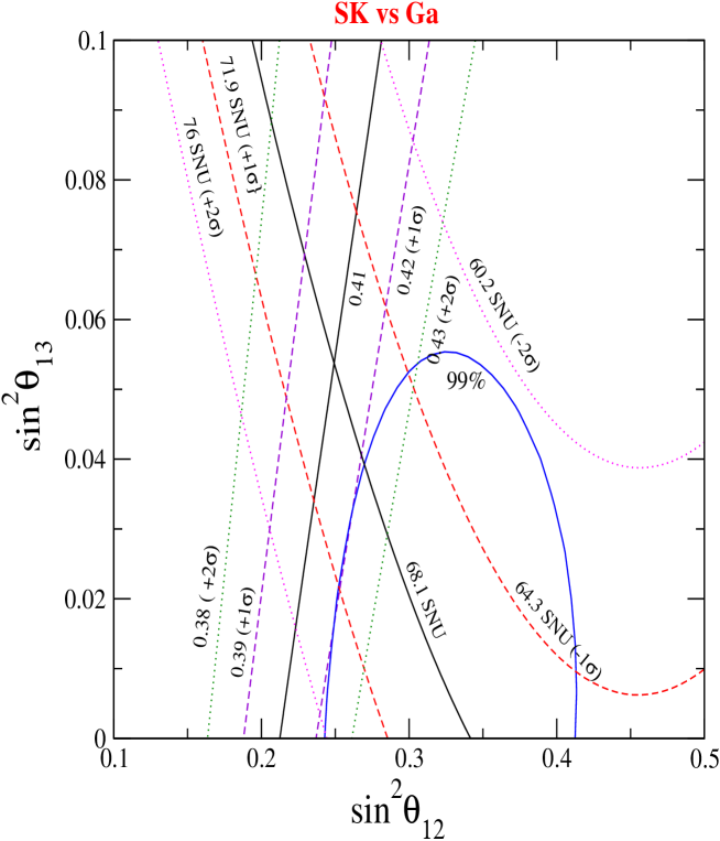
The iso-contours of the SK rate in the plane are presented in fig. 4 for . They correspond to the SK central value as well as the 1 and 2 deviations. According to fig. 4, for the ratio is achieved at which is about below the best global value. In turn, the best global value and lead to .
With decrease of the corresponding iso-contours shift to larger and smaller . For arbitrary one can still use the grid of contours calculated for , but with changed values . Indeed, according to (69), for given values and one should take the contour .
The combination of SK- and Ga- data
(crossing point of the contours which correspond
to the central experimental values) selects
as is seen from fig. 4.
For the best fit SK value, ,
corresponds to the iso-contour with . The intersection of this contour
with the iso-contour SNU occurs at
much smaller 1-3 mixing: .
4). The Argon production rate in the Homestake experiment is determined by
| (70) |
According to the SSM is dominated by the high energy (boron) neutrinos. Therefore the contours of constant rate (fig. 5) have typical slope of the high energy observables. We show these contours for .
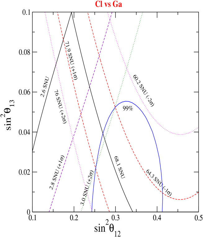
For and the best global value of the rate is about 3.15 SNU which is above the experimental result. The combination of Cl- and Ga-results prefers large 1-3 mixing: which deviates from zero by .
For the arbitrary again one needs to rescale
. Thus, for
and SNU the iso-contour with
SNU should be used. It intersects with
iso-contour SNU at .
Summarizing, for eV2, the combination of SNO and Ga data selects , which is practically independent of . For (which follows from the global fit) the combination of SK and Ga results leads to and the combination of Cl and Ga data selects , however statistical significance of the latter is low. The average from these three combinations is about . It agrees well with results of fit of all the solar data for the same . For larger the larger values of would be preferable.
Notice that available spectral information does not give strong
restriction on .
In fact, flatness of the
measured spectrum of events at SNO and SK may even favor non-zero
.
Indeed, at high energies an increase of implies
increase of and therefore flattening of the spectrum.
The results on 1-3 mixing described above are in agreement with
the best fit value from the global analysis of all solar
neutrino data, ,
which is realized, however, for smaller (62).
Inclusion of the CHOOZ result diminishes
to practically zero.
Let us consider dependence of the iso-contours on . Using (55) we find for the high energy part:
| (71) |
where we have expressed in terms of .
In fig. 6 we show results of numerical
computations
of the iso-contours for Ga-rate and CC/NC ratio for three different
values of . In agreement with our qualitative
consideration a shift of the low energy contours is much weaker.
Variations of from to
eV2 (which is about 25% change) gives
and
.
Reduction of the uncertainty in down to 14% will result
in and
.
This is much smaller than the expected sensitivity of future solar
neutrino studies. The contours have been obtained for
. We have found that variations of
produce shift of the Ge-lines by ,
and the SNO contours do not change at all.
Let us consider the effect of matter corrections to the 1-3 mixing. As we have established in sec. 2, the effect is reduced to renormalization of according to Eq. (40). True value of is smaller than the one extracted from the data without taking into account matter correction. The renormalization is negligible for the low energy observables and it is of the order 5% at high energies. So, the iso-contours of high energy observables should be shifted down by factor . This, in turn leads to decrease of in the intersection points: e.g., instead of one finds 0.016.
The figures presented in this section allow us to estimate relevance of the non-zero 1-3 mixing for the solar neutrino.
For a given CC/NC ratio an increase of from 0 to 0.05 ( upper bound) corresponds to decrease the Ge-production rate by or SNU. Inversely, for a given , the same increase of leads to decrease of the ratio CC/NC: CC/NC . The same change of diminishes the SK rate by : . So, the variations of produce about or smaller variations of observables. As we have discussed in the beginning of previous section, the impact of on the global fit of the solar neutrino data is much weaker: increase of leads to only increase of .
6 Sensitivity of the future solar neutrino experiments to 1-3 mixing
As we have shown, some sensitivity of the solar neutrino data
to the 1-3 mixing appears essentially due
to the combination of the SNO- and SK- results from the one hand side and
the Gallium results from the other side.
Future high precision measurements will have better sensitivity.
To evaluate this sensitivity and to
study possible implications of measurements we have constructed
fine grids of the iso-contours of various observables.
We will use the expected errors, , in
determination of as a measure of the sensitivity.
and errors can also be estimated from the
grids of iso-contours we present. In the first approximation
error is given by .
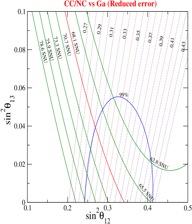
1). In fig. 7 we show the fine grid of iso-contours for the CC/NC-ratio and the Ge- production rate. The SNO (phase III) will measure the NC- event rate with 6% accuracy [53]. If we assume a reduced error of 5% for the CC-data then this makes the CC/NC error as 8% which can be compared to the present error of 11%. (This corresponds to reduction of the absolute error in the CC/NC ratio down to 0.024 from the current value of 0.035.)
According to fig. 7, the current Ge-production rate accuracy is SNU. Using this accuracy and the expected SNO-III error, we find from fig. 7 the sensitivity ( error) to in the region :
| (73) |
It is only slightly better than the present one (67).
If we take 5% accuracy for future possible measurements of CC/NC ratio and the Ge-production rate error 2.6 SNU (the later is slightly larger than the present systematic error [47], and it could correspond to future hypothetical large mass Gallium experiment for which statistical error is substantially smaller than the systematic one; this can be considered as the ultimate sensitivity of the Gallium experiments), then according to fig. 7
| (74) |
In this case the value would have
only significance, and in the case of very small
the upper bound will
be
at .
2). The Borexino and KamLAND plan to measure signal from the neutrinos. The iso-contours can be well described by the low energy formula (58). Taking into account contribution from the non-electron (converted) neutrinos we find the iso-contours, , which coincide with iso-contours , where .
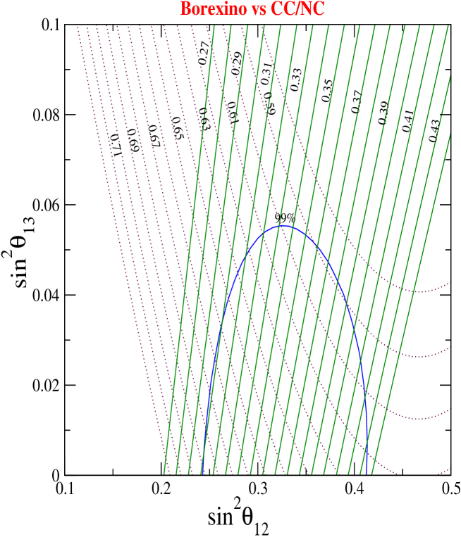
The results of calculations are shown in fig. 8. The Borexino contours have similar form to those for Ga-rate.
Borexino is expected to accumulate 44000 events in 4 years of time
( 30 events/day) for LMA MSW solution. This corresponds to a
statistical error of only 0.5% [54]. But
the accuracy of measurement will be dominated by the
background and systematics.
Furthermore, the SSM prediction for the flux has 10% uncertainty
which will add to the total error unless one keeps
the normalization of flux as a free parameter
to be determined from the Borexino experiment itself with a higher
accuracy.
Using fig. 8 we estimate that
a 5% accuracy of measurements of the rate at Borexino
will contribute to improvement of
sensitivity of the solar studies to .
3). New low energy solar neutrino experiments will be able to measure the pp-neutrino flux with high accuracy [55]. Two kinds of experiments are being discussed [56]: one – using the charged current reactions (LENS, MOON, SIREN) and the other – using the neutrino-electron scattering process (XMASS, CLEAN, HERON, MUNU, GENIUS).
For the pp-neutrinos we can use the iso-contour equation for the low energies as in (58) with substitution and . Practically, is negligible.
In fig. 9 we show the contours of constant rate of the scattering events due to the pp-neutrinos. The neutral current contribution is also included. According to fig. 9, future measurements of the CC/NC ratio with 5% accuracy and the pp-rate with 2% accuracy will have a sensitivity ( error)
| (75) |
Consequently, the value will be established
with significance, and in the case of very small
the upper bounds
at can be achieved.
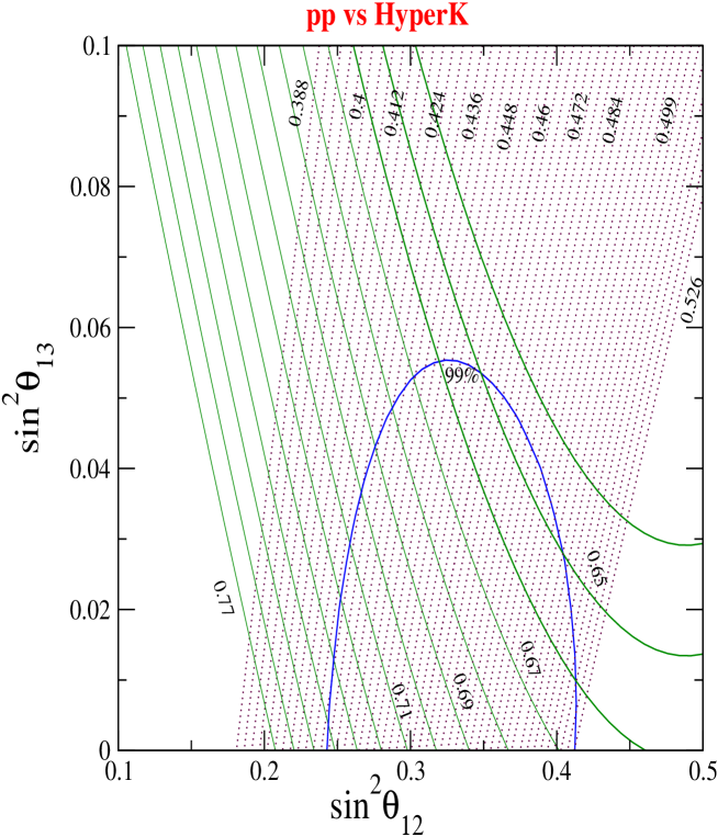
4). Future Megaton scale water Cherenkov detectors HyperKamiokande [57] and UNO [58] will be able to measure the ratio with accuracy . We construct the fine grid of the iso-contours for (fig. 10). According to fig. 10 these measurements of and the pp-rate (2% accuracy) would have a sensitivity ( error)
| (76) |
However, the problem here is the poor knowledge of . It is difficult to expect that accuracy of the theoretical predictions will be better than 10%. Comparable accuracy will be achieved in the direct measurements of the neutral currents. The global fit of the data which include the spectral information and the regeneration effect with free may give better accuracy.
So, we conclude that the future solar neutrino studies
may reach a sensitivity
(), as compared with the present sensitivity
0.05 - 0.06. It seems that even combined fit of several future
precision measurements will not go down to 0.01 which may be
considered as an ultimate sensitivity
of solar neutrino measurements of .
On the basis of studies performed in secs. 5 and 6 we can identify signatures of the non-zero . In general, they show up as a mismatch of the low and high energy measurements. The signatures include
-
•
Small value of the Ge production rate . For a given ratio CC/NC one can find the critical value of , so that inequality
(77) will testify for the non-zero value of . From the fig. 7 we find SNU, SNU, SNU, SNU, etc.. The larger the difference in (77), the larger . In fact, the present data satisfy the inequality (77), however the statistical significance is low. Apparently if CC/NC and are measured with high accuracy, the presence of non-zero can be established.
The inequality (77) can be inverted, so that small values of CC/NC for a given ,
(78) testify for non-zero .
-
•
Small Borexino rate:
(79) The critical Borexino rates for different values of CC/NC equal: , , , , .
-
•
Small event rate produced by the pp-neutrinos:
(80) According to fig. 10 the critical values equal 0.75 (0.294), 0.73(0.318), 0.71(0.343), 0.69(0.373).
-
•
Weak spectrum distortion of the boron neutrinos. The spectrum distortion can be characterized, e.g., by the ratio of suppressions at low and hight energies . There is certain critical value of the distortion, , which depends on CC/NC, so that weaker distortion will testify for non-zero 1-3 mixing. Indeed, for fixed CC/NC with increase of , the 1-2 mixing, , should increase (45) and therefore, the up turn of spectrum at low energies should be weaker.
7 Implications of the solar neutrino measurements of
Let us first compare sensitivities of the future solar neutrino experiments and future reactor and accelerator experiments given in eqns. (4, 5, 6). With the expected accuracy of SNO-III and 2% accuracy of the pp-neutrino flux measurements the solar neutrino experiments can reach sensitivity comparable to the one of the forthcoming MINOS and CNGS experiments. This sensitivity is at the level of the present bound from the global fit of all oscillation data and it is certainly lower than the sensitivity of future measurements.
The solar neutrino sensitivity would be comparable to that of J-PARC and Double-CHOOZ if the pp-neutrino flux is measured with 1% accuracy and CC/NC ratio - with 3% accuracy which looks rather unrealistic now.
Notice that the survival probability does not depend on the CP phase , and therefore the problem of degeneracy with [59] does not arise. So, the solar neutrinos studies can provide a clean channel for determination of like the reactor neutrinos. Therefore, in spite of the lower sensitivity the solar neutrino data will contribute somehow to resolution of degeneracy of these parameters in the future global fits.
It seems that the reactor and accelerator experiments will obtain results much before future high statistics solar neutrino experiments will start to operate. In this case possible implications of the solar neutrino measurements can include
1). Precise determination of : resolution of the degeneracy.
2). Comparison of results on (as well as on ) from the solar neutrinos and reactor/accelerator experiments. The outcome could be further confirmation of the reactor/accelerator results by solar neutrinos, or establishing certain discrepancy which may imply new physics beyond the LMA solution of the solar neutrino problem.
Let us consider these two points in some details.
1). Resolving degeneracy of angles.
Due to the strong
degeneracy
unknown value of leads to uncertainty in
the determination of and vice-versa.
Thus, in the CC/NC measurements, inclusion of the 1-3 mixing produces an
increase of by (that is, by 20%)
if increases from 0 to 0.06
(see fig. 7).
In the pp-neutrino flux measurements decreases by
, when increases from 0 to 0.06 (see
fig. 9).
So, precise determination of
() from the solar neutrino data
is not possible unless ()
is measured or
strongly restricted.
As follows from our analysis a combination of high statistics measurement
at high and low energies can remove the degeneracy.
2). Confronting the solar and reactor/accelerator results. If non-zero is measured, our analysis will allow to understand relevance of the 1-3 mixing to the precision solar neutrino studies. For fixed , the 1-3 mixing will change determination of .
Notice that dependence of sensitivity of the solar neutrino studies
to
on the mass is very weak (via matter corrections to
1-3 mixing) in contrast to
laboratory measurements. So, for small the former
will have some advantage.
If effect is not found in future laboratory experiments
and the upper bound at the level is
established, the effect of 1-3 mixing will be irrelevant even for
measurements with the 1% accuracy. The uncertainty of future
measurements of due to unknown
will be reduced down to 0.01. Furthermore, the
precise measurements of by CC/NC will have
the smallest uncertainty due to larger slope of the iso-lines.
The analysis performed in this paper will allow us to understand new physics if inconsistencies in results of measurements will show up. Implications will depend on character of results, and in the positive case, on particular value of . Comparing the laboratory bound with the results of solar neutrino studies one can realize new physics effects which may show up in the solar neutrinos only and can not be found otherwise. Let us consider some examples.
Suppose that in the standard analysis precision solar neutrino measurements will give a nonzero value of which is larger than the upper bound from the reactor/accelerator experiments. Such a situation may indicate some additional suppression of the solar neutrino flux at low energies. Indeed, this would shift the low iso-contours to the left - down. It would be equivalent of taking the low iso-contours in our plots (e.g., in fig. 3) with larger survival probability. The intersection with high energy iso-contours will shift down and therefore the inferred value of will be reduced. This situation can be reproduced in the presence of sterile neutrino with eV2 [60]. In this case the extracted value of reduces too.
Agreement between the solar and laboratory measurements can be also achieved by an additional suppression of the high energy (boron) flux due to flavor conversion, so that CC/NC lines move to the right - down. In this case also the intersection of the high and low iso-contours moves down and the inferred value of increases. Such an effect can be produced by certain non-standard neutrino interactions.
The value of extracted from the solar neutrino
studies can be diminished if both the low and high energy fluxes are
reduced
by some additional mechanism. In fact, this imitates the effect of the
1 - 3 mixing and can be achieved by additional non-standard interactions.
Let us consider the opposite situation:
is discovered in the reactor/accelerator
experiments, but the solar neutrino data prefer zero or smaller
value of .
This can be explained if the survival probability is larger
than the one predicted for given values of
and . Again some scenarios
with modified dynamics of conversion due to new interactions of
neutrinos can reproduce such a situation.
Similarly discrepancy can be realized comparing values of the 1-2 mixing extracted from the solar neutrino data and reactor/accelerator experiments. Indeed, the can be measured with 3% accuracy at (1 d.o.f.) in the reactor experiments with baseline 50 - 70 km [61, 62, 43] provided that the 1-3 mixing is determined (restricted) accurately enough from independent measurements. Since a non-zero drives the 1-2 mixing to smaller values in such an experiment, combination with high energy solar neutrino experiments for which non-zero drives to higher values can resolve the degeneracy. This is similar to combination of low energy and high energy solar neutrino experiments as discussed in the present article. In this case one can compare the () allowed regions from the solar neutrino studies and from reactor experiments.
8 Conclusion
1). We have derived formula for the survival probability in
the three neutrino context (35) which includes all
corrections relevant for the future precision of measurements.
We estimated the accuracy of approximation made.
2). In the three generation context in the first approximation
(neglecting the matter effect on )
the solar neutrino probabilities are functions of the mass split
and the mixing angles:
and .
The split is already determined with a high precision
by current data. Furthermore, the survival probability has a weak
dependence on in the allowed region.
In view of this we have constructed various plots in plane which clearly demonstrate the
degeneracy of these mixing angles and also show how the uncertainty
in one is going to affect the precision determination of the other.
Synergy between the high and low energy solar neutrino
flux measurement provides a better constraint on and allows us
to resolve the degeneracy of these mixing angles.
3). Among the existing solar neutrino experiments only the Ga-experiment is sensitive to the low energy part of the spectrum and in particular to the pp-neutrinos. Therefore we construct the iso-rates for Ga experiments in the plane and investigate how the combinations of these with the iso-rates of Cl, SK and CC/NC ratio in SNO constrain .
At present the sensitivity of the solar neutrino experiments to is rather weak and no indications of non-zero value has been obtained. Our analysis of all solar neutrino data leads to statistically insignificant non-zero best fit value: . Similar value, , follows from the fit of the solar neutrino data for eV2 selected by the KamLAND experiment. The combination of the CC/NC ratio at SNO and rate, which are essentially independent of the solar neutrino fluxes, gives ().
The global fit of all existing data (including
reactor, accelerator and atmospheric neutrino results) leads to as
the best fit point and to the upper bounds
at from the two parameter plots in
plane.
4). The precision of determination will improve with future accurate measurements of the pp-neutrino flux, the CC/NC ratio and the energy spectrum of events at MeV. We find that measurements with 5% error in the CC/NC ratio and 2% error in the pp-neutrino flux in scattering will have a sensitivity ( error) (). The value () looks like the ultimate sensitivity which could be reached in the solar neutrino experiments of the next generation.
Since the probability involved is the problem of
degeneracy with CP phase does not appear and solar
neutrinos can provide a clean channel for measurements
like the reactor neutrinos.
5). It is likely that new accelerator and reactor results will be obtained first. Comparison of the results from solar neutrinos and accelerator/reactor experiments may confirm each other and further improve determination of or reveal some discrepancy which will indicate a new physics beyond usual interpretation of the solar neutrino anomaly.
Determination of will eliminate or reduce the degeneracy thus improving measurements of 1-2 mixing. Inversely, the better determination of can help in improving the precision of the measurements in the solar neutrino studies.
Comparison of the results of (as well as ) measurements in solar neutrinos and in reactor and accelerator experiments may uncover new interesting physics beyond LMA MSW picture which can not be found otherwise.
S.G. would like to thank The Abdus Salam International Centre for Theoretical Physics for hospitality and A. Bandyopadhyay and S. Choubey for using some of the codes developed with them. The authors are grateful to E. Lisi for valuable comments.
References
- [1] M. Apollonio et al., Phys. Lett. B466 (1999) 415; Eur. Phys. J. C 27 (2003) 331.
- [2] F. Boehm et al., Phys. Rev. D62 (2000) 072002.
- [3] G. L. Fogli, E. Lisi, A. Marrone and A. Palazzo, arXiv:hep-ph/0506083.
- [4] A. Strumia and F. Vissani, arXiv:hep-ph/0503246.
- [5] J. N. Bahcall, M.C. Gonzalez-Garcia C. Pena-Garay, JHEP 0408, 016 (2004); [hep-ph/0406294].
- [6] A. Bandyopadhyay et al., hep-ph/0406328.
- [7] M. Maltoni, T. Schwetz, M.A. Tortola, J.W.F. Valle, New J. Phys. 6 122 (2004), [hep-ph/0405172] v.3.
- [8] M. C. Gonzalez-Garcia, [hep-ph/0410030].
- [9] S. Goswami, talk at Neutrino 2004, Paris, http://neutrino2004.in2p3.fr, [hep-ph/0409224].
- [10] R. Saakian, Nucl. Phys. Proc. Suppl. 111, 169 (2002).
- [11] http://proj-cngs.web.cern.ch/proj-cngs/.
- [12] http://jkj.tokai.jaeri.go.jp/.
- [13] P. Huber, M. Lindner, T. Schwetz and W. Winter, Nucl. Phys. B 665 (2003) 487 [hep-ph/0303232].
- [14] Letter of Intent for Double-CHOOZ F. Ardellier et. al., hep-ex/0405032.
- [15] H. Minakata, H. Sugiyama, O. Yasuda, K. Inoue and F. Suekane, Phys. Rev. D 68, 033017 (2003) [arXiv:hep-ph/0211111];
- [16] C. Lunardini and A. Y. Smirnov, JCAP 0306, 009 (2003) [hep-ph/0302033].
- [17] G. L. Fogli, E. Lisi, A. Mirizzi and D. Montanino, Nucl. Phys. Proc. Suppl. 145, 343 (2005).
- [18] M. Lindner, Int. J. Mod. Phys. A18, 3921, (2003) and references therein.
- [19] G. L. Fogli, E. Lisi, A. Marrone, D. Montanino, A. Palazzo, [hep-ph/0104221].
- [20] G.L. Fogli, G. Lettera, E. Lisi, A. Marrone, A. Palazzo, A. Rotunno, Phys. Rev. D66, 093008, (2002), G.L. Fogli, E. Lisi, A. Marrone, D. Montanino, A. Palazzo, A.M. Rotunno, Phys. Rev. D69, 017301, (2004) [hep-ph/0308055].
- [21] J. N. Bahcall and C. Pena-Garay, JHEP 0311, 004 (2003) [hep-ph/0305159].
- [22] M. C. Gonzalez-Garcia, C. Pena-Garay, Phys. Lett. B527 199, (2002).
- [23] M.C. Gonzalez-Garcia, C. Pena-Garay, Phys. Rev. D68 093003 (2003).
- [24] A. B. Balantekin, H. Yuksel, J. Phys. G29 665 (2003).
- [25] M. Maltoni, T. Schwetz, M.A. Tortola, J.W.F. Valle, Phys. Rev. D 68, 113010 (2003), M.C. Gonzalez-Garcia, M. Maltoni, C. Pena-Garay, J.W.F. Valle, Phys. Rev. D 63 033005 (2001).
- [26] P. C. de Holanda, A.Yu. Smirnov, Astropart. Phys. 21, 287, (2004) [hep-ph/0309299].
- [27] P. C. de Holanda, A.Yu. Smirnov, JCAP 0302, 001, (2003); P.C. de Holanda, A.Yu. Smirnov, Phys. Rev. D66, 113005, (2002).
- [28] A. Bandyopadhyay, S. Choubey, S. Goswami and K. Kar, Phys. Rev. D 65 (2002) 073031 [hep-ph/0110307].
- [29] A. Bandyopadhyay, S. Choubey, R. Gandhi, S. Goswami and D. P. Roy, J. Phys. G 29, 2465 (2003) [hep-ph/0211266]. A. Bandyopadhyay, S. Choubey, R. Gandhi, S. Goswami and D. P. Roy, Phys. Lett. B 559, 121 (2003) [arXiv:hep-ph/0212146].
- [30] A. Bandyopadhyay, S. Choubey, S. Goswami, S.T. Petcov, D.P. Roy, Phys. Lett. B583, 134 (2004).
- [31] S. C. Lim, In Proc. of BNL Neutrino Workshop, Upton, NY, USA 1987, edited by M. Murtagh, BNL-52079, C87/02/05.
- [32] X. Shi, D. N. Schramm, Phys. Lett. B 283, 305 (1992), X. Shi, D.N. Schramm, J. N. Bahcall, Phys. Rev. Lett. 69, 717 (1992).
- [33] G. L. Fogli, E. Lisi, A. Palazzo, Phys. Rev. D 65, 073019 (2002), [hep-ph/0105080].
- [34] C.S. Lim, K. Ogure, H. Tsujimoto, Phys. Rev. D67, 033007 (2003), [hep-ph/0210066].
- [35] M. Blennow, T. Ohlsson and H. Snellman, Phys. Rev. D69, 073006 (2004), [hep-ph/0311098].
- [36] E. Kh. Akhmedov, M. A. Tortola, J.W.F. Valle, JHEP 0405, 057 (2004), [hep-ph/0404083].
- [37] S. P. Mikheyev and A. Yu. Smirnov, Yad. Fiz. 42, 1441 (1985) [ Sov. J. Nucl. Phys. 42, 913 (1985)]; Nuovo Cim. C9, 17 (1986); S. P. Mikheyev and A. Yu. Smirnov, ZHETF, 91, (1986), [Sov. Phys. JETP, 64, 4 (1986)] (reprinted in ”Solar neutrinos: the first thirty years”, Eds. J.N.Bahcall et. al.).
- [38] A. Messiah, in Proceedings of the th Moriond Workshop On Massive Neutrino in Particle Physics and Astrophysics, ed. O. Fackler and J. Tran Thanh Van, (1986) p.373.
- [39] W. Haxton, Phys. Rev. Lett. 57 (1986) 1271; S. J. Parke, Phys. Rev. Lett. 57(1986) 1275.
- [40] P. C. de Holanda, W. Liao and A. Y. Smirnov, Nucl. Phys. B702, 307, (2004), [hep-ph/0404042].
- [41] A. N. Ioannisian and A. Y. Smirnov, Phys. Rev. Lett. 93 (2004) 241801.
- [42] M. C. Gonzalez-Garcia, C. Pena-Garay and A. Y. Smirnov, Phys. Rev. D 63 (2001) 113004.
- [43] A. Bandyopadhyay, S. Choubey, S. Goswami and S. T. Petcov, [hep-ph/0410283].
- [44] E. Kearns, talk at Neutrino 2004, Paris, http://neutrino2004.in2p3.fr.
- [45] T. Araki et al., [KamLAND Collaboration], hep-ex/0406035 (v3).
- [46] B. T. Cleveland et al., Detector,” Astrophys. J. 496, 505 (1998).
- [47] J. N. Abdurashitov et al. [SAGE Collaboration], J. Exp. Theor. Phys. 95, 181 (2002) [Zh. Eksp. Teor. Fiz. 122, 211 (2002)] [arXiv:astro-ph/0204245]. W. Hampel et al. [GALLEX Collaboration], Phys. Lett. B 447, 127 (1999) ; M. Altmann et al. [GNO Collaboration], Phys. Lett. B 616 (2005) 174.
- [48] S. Fukuda et al. [Super-Kamiokande Collaboration], Phys. Lett. B 539, 179 (2002), [hep-ex/0205075].
- [49] Q. R. Ahmad et al. [SNO Collaboration], Phys. Rev. Lett. 89, 011302 (2002) [nucl-ex/0204009]. S. N. Ahmed et al. [SNO Collaboration], Phys. Rev. Lett. 92, 181301 (2004) [arXiv:nucl-ex/0309004].
- [50] B. Aharmim et al. [SNO Collaboration], arXiv:nucl-ex/0502021.
- [51] J. N. Bahcall and M. H. Pinsonneault, Phys. Rev. Lett. 92, 121301 (2004) [astro-ph/0402114].
- [52] J. N. Bahcall, S. Basu and A. M. Serenelli, arXiv:astro-ph/0502563.
- [53] K. Graham, talk at NOON 2004, February 11-15, 2004, Tokyo, Japan, http://www-sk.icrr.u-tokyo.ac.jp/noon2004/; H. Robertson for the SNO Collaboration, Talk given at TAUP 2003, Univ. of Washington, Seattle, Washington, September 5 - 9, 2003, http://mocha.phys.washington.edu/taup2003
- [54] C. Galbiati, talk at Neutrino 2004, Paris, http://neutrino2004.in2p3.fr.
- [55] M. Nakahata, Talk given at the Int. Workshop on Neutrino Oscillations and their Origin (NOON2004), February 11 - 15, 2004, Tokyo, Japan; S. Schönert, talk at Neutrino 2002, Munich, Germany,
- [56] see e.g., Y. Suzuki, Nucl. Phys. B (Proc. Suppl.) 143, 27 (2005) “Neutrino 2004”
- [57] T. Nakaya, Nucl. Phys. B (Proc. Suppl.) 118, 210 (2003) “Neutrino-2002” K. Nakamura, talk at the workshop “Neutrinos and Implications for Physics Beyond the Standard Model” 2002, http://insti.physics.sunysb.edu/itp/conf/neutrino/talks/nakamura.pdf.
- [58] UNO Proto-collaboration, UNO Whitepaper: Physics Potential and Feasibility of UNO, SBHEP-01-03(2000), http://nngroup.physics.sunysb.edu/uno/; see also C. K. Jung 2002, hep-ex/0005046.
- [59] V. Barger, D. Marfatia and K. Whisnant, Phys. Rev. D 65, 073023 (2002) [hep-ph/0112119].
- [60] P. C. de Holanda and A. Y. Smirnov, Phys. Rev. D 69, 113002 (2004) [hep-ph/0307266].
- [61] A. Bandyopadhyay, S. Choubey and S. Goswami, Phys. Rev. D 67, 113011 (2003).
- [62] H. Minakata, H. Nunokawa, W. J. C. Teves and R. Zukanovich Funchal, [hep-ph/0407326].