Chiral symmetry and density wave in quark matter

Abstract

A density wave in quark matter is discussed at finite temperature, which occurs along with the chiral condensation, and is described by a dual standing wave in scalar and pseudo-scalar condensates on the chiral circle. The mechanism is quite similar to that for the spin density wave suggested by Overhauser, and entirely reflects many-body effects. It is found within a mean-field approximation for NJL model that the chiral condensed phase with the density wave develops at a high-density region just outside the usual chiral-transition line in phase diagram. A magnetic property of the density wave is also elucidated.

I Introduction

In a recent decade the condensed matter physics of QCD has been an exciting area in nuclear physics. In particular, its phase structure at finite-density and relatively low-temperature region is studied actively, since it was suggested that the color superconductivity (CSC) involved observable consequence of quark matter due to the large magnitude of its gap energy over a few hundred MeV csc0 ; csc1 ; csc2 . Although QCD at finite densities has important implications for physics in other fields, e.g., the core of the compact stars and their evolution nutr1 , it remains in not understood adequately.

Whereas the quark Cooper-pair (p-p) condensations attracts much interest, particle-hole (p-h) condensations, which are related to the chiral condensation csc1 ; csc2 or ferromagnetism in quark matter tat ; nak ; ferr1 , have also been studied, and their interplay with CSC has been discussed. Since the Cooper instability on the Fermi surface occurs for arbitrarily weak interaction, the p-p condensation should dominate at asymptotically free high-density limit. While on the other hand, there exists a critical strength of the interaction in the p-h channel for its condensation.

At moderate densities, however, where the interaction is strong enough, p-p and p-h condensations are competitive, and various types of the p-h condensations are proposed der1 ; der2 in which the p-h pairs in scalar or tensor channels have a finite total momentum indicating standing waves. Instability for the density wave in quark matter was first discussed by Deryagin et al. der0 at asymptotically high densities where the interaction was very weak, and they concluded that the density-wave instability prevailed over the Cooper’s one in the large $N_{c}$ (the number of colors) limit due to the dynamical suppression of colored p-p pairings.

In general, the density waves are favored in one-dimensional (1-D) systems, and have the wavenumber $Q=2k_{F}$ according to the Peierls instability kagoshima ; peiel1 , e.g., charge density waves in quasi-1-D metals peiel2 . The essence of its mechanism is the nesting of Fermi surfaces and the level-repulsion (crossing) of single particle spectra due to the p-h interaction with the finite total wavenumber. Thus the low dimensionality has a essential role to make the density-wave states stable. In higher dimensional systems, however, the transition occurs provided the interaction of a corresponding (p-h) channel is strong enough. For the 3-D electron gas, it was shown by Overhauser ove ; sdw1 that the paramagnetic state was unstable with respect to formation of a static spin density wave (SDW), in which spectra of up- and down-spin states deform to bring about a level-crossing due to the Fock exchange interactions, while the wavenumber does not precisely coincide with $2k_{F}$ because of incomplete nesting in the higher dimension.

In the recent paper LettCDCW , we suggested a density wave in quark matter at moderate densities in analogy with SDW mentioned above. It occurs along with the chiral condensation and is represented by a dual standing wave in scalar and pseudo-scalar condensates (we have called it ‘dual chiral-density wave’, DCDW). The DCDW has different features in comparison with the previously discussed chiral-density waves der0 ; der1 ; der2 , and emerges at a moderate density region $\rho_{B}/\rho_{0}\simeq 3-6$ (where $\rho_{0}=0.16{\rm fm}^{-3}$, the normal nuclear matter density).

In this paper we would like to further discuss DCDW and figure out the mechanism in detail. We also present a phase diagram on the density-temperature plane. In Sec. II we start by introducing the order parameters for the dual chiral-density wave and show the nature of the ground state on the analogy of the spin density wave: a level-crossing of single-particle spectrum in the left- and right-handed quarks. Sec. III is devoted to concrete calculations by use of Nambu-Jona-Lasinio (NJL) model nam to present a phase diagram at finite density and temperature, in the case of 2 flavors and 3 colors. In Sec. IV we summarize and give some comments on outlooks.

II Nature of dual chiral-density wave

In the pioneering studies of chiral density waves der0 ; der1 ; der2 , a spatial modulation in the chiral condensation was considered; the scalar condensation with a wavenumber vector ${\bf q}$ occurs, $\langle\bar{\psi}\psi\rangle\propto\cos({\bf q}\cdot{\bf r})$. In this section, we consider a directional modulation with respect to the chiral rotation, since the directional excitation modes should be lower than the radial ones in the spontaneously symmetry-broken phases. We propose the dual chiral-density wave (DCDW) in scalar and pseudo-scalar condensation,

$$\langle\bar{\psi}\psi\rangle = \Delta\cos({\bf q}\cdot{\bf r}),$$

$$\langle\bar{\psi}i\gamma_{5}\psi\rangle = \Delta\sin({\bf q}\cdot{\bf r}),$$ (1)

where the amplitude $\Delta$ corresponds to the magnitude of the chiral condensation; $\langle\bar{\psi}\psi\rangle^{2}+\langle\bar{\psi}i\gamma_{5}\psi\rangle^{2}=\Delta^{2}$.

We give the single-particle spectrum, in the presence of the density wave (1) as an external field. The Lagrangian density of the system in the chiral limit then reads

$${\cal L} = \bar{\psi}(r)\left[i/{\!\!\!}{\partial}+2G\Delta\left\{\cos({\bf q}\cdot{\bf r})+i\gamma_{5}\sin({\bf q}\cdot{\bf r})\right\}\right]\psi(r),$$ (2)

where $2G$ is a coupling constant between the quark and DCDW. In the chiral representation, it becomes clear how the density wave affects the quark fields: the Lagrangian shows that the density wave connects left- and right-handed particles in pairs with the total momentum ${\bf q}$,

$$\int{\rm d}^{3}r{\cal L} = \int\frac{{\rm d}^{3}p}{(2\pi)^{3}}\left(\begin{array}[]{c}\psi_{L}(p-q/2)\\ \psi_{R}(p+q/2)\end{array}\right)^{\dagger}\left(\begin{array}[]{cc}\bar{\sigma}_{\mu}(p-q/2)^{\mu}&-M\\ -M&\sigma_{\mu}(p+q/2)^{\mu}\end{array}\right)\left(\begin{array}[]{c}\psi_{L}(p-q/2)\\ \psi_{R}(p+q/2)\end{array}\right),$$ (9)

where $q^{\mu}=(0,{\bf q})$, and $M$($\equiv-2G\Delta$) corresponds to the dynamical mass if the density wave is generated by quark interactions as the mean-field. The single-particle (quasi-particle) spectrum is obtained from the poles of the propagator:

$$\det{\left[\bar{\sigma}_{\mu}(p-q/2)^{\mu}\sigma_{\mu}(p+q/2)^{\mu}-M^{2}\right]}=0.$$ (10)

From the above equation we found the spectrum: positive and negative energies, $E_{\pm}({\bf p})$ and $-E_{\pm}({\bf p})$,

$$E_{\pm}({\bf p})=\sqrt{E_{0}({\bf p})^{2}+|{\bf q}|^{2}/4\pm\sqrt{({\bf p}\cdot{\bf q})^{2}+M^{2}|{\bf q}|^{2}}},~{}~{}~{}E_{0}(p)=(M^{2}+|{\bf p}|^{2})^{1/2}.$$ (11)

Because of the finite ${\bf q}$ and $\Delta$, the spectrum is deformed and split into two branches denoted by $E_{\pm}({\bf p})$, as shown in Fig. 1 where the direction of ${\bf q}$ is taken parallel to the $z$ axis. The two branches exhibit a level-crossing between the left- and right-handed particles.

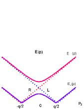
Figure 1: Two branches of the single-particle spectrum (11) are plotted along $p_{z}$ axis at $p_{x}=p_{y}=0$ where ${\bf q}//\hat{z}$. Dashed (Solid) lines correspond to $M=0$ ($M\neq 0$).

For ${\bf q}=(0,0,q)$, the corresponding eigen spinors are given, in the chiral representation, by

$$u_{\pm}({\bf p}) \equiv \mathcal{N_{\pm}}\left(\begin{array}[]{c}\psi_{L}^{(\pm)}({\bf p}-{\bf q}/2)\\ \psi_{R}^{(\pm)}({\bf p}+{\bf q}/2)\end{array}\right)~{}~{}\mbox{for positive energy }E_{\pm}({\bf p}),$$ (14)

$$v_{\pm}({\bf p}) \equiv u_{\pm}({\bf p})|_{E_{\pm}({\bf p})\rightarrow-E_{\pm}({\bf p})}~{}~{}\mbox{for negative energy}-E_{\pm}({\bf p}),$$ (15)

where $\mathcal{N_{\pm}}$ is a normalization factor for $u_{\pm}^{\dagger}u_{\pm}=v_{\pm}^{\dagger}v_{\pm}=1$, and

$$\psi_{R}^{(\pm)}({\bf p}+{\bf q}/2) = \left(\begin{array}[]{c}\frac{\pm\sqrt{p_{z}^{2}+M^{2}}+q/2+E_{\pm}({\bf p})}{p_{x}+ip_{y}}\\ 1\end{array}\right),$$ (18)

$$\psi_{L}^{(\pm)}({\bf p}-{\bf q}/2) = \frac{M}{p_{z}\pm\sqrt{p_{z}^{2}+M^{2}}}~{}\sigma_{3}~{}\psi_{R}^{(\pm)}({\bf p}+{\bf q}/2).$$ (19)

Here it should be noted that the original spinor in eq. (2), $\psi(r)$, is represented as a plane wave expansion for the eigen spinors in eqs. (14)-(15):

$$\psi(r)=e^{-i\gamma_{5}{\bf q}\cdot{\bf r}/2}\sum_{s=\pm}\int\frac{{\rm d}^{3}p}{(2\pi)^{3}}\left\{a_{s}({\bf p})u_{s}({\bf p})+b_{s}({\bf p})v_{s}({\bf p})\right\}e^{-ip\cdot r}\equiv e^{-i\gamma_{5}{\bf q}\cdot{\bf r}/2}\int\frac{{\rm d}^{3}p}{(2\pi)^{3}}\tilde{\psi}(p)e^{-ip\cdot r},$$ (20)

where $a_{\pm}({\bf p})$ ($b_{\pm}({\bf p})$) is annihilation operator for the positive (negative) quasi-particle state. The factor, $\exp(-i\gamma_{5}{\bf q}\cdot{\bf r}/2)$, comes from the momentum shifts $\mp q/2$ in the left- and right-handed particles in eq. (9) due to the presence of DCDW, and thus reflects a nature of the spatially chiral-rotated ground state. The factor corresponds also to a kind of Weinberg transformation, which changes the system from spatially modulated one to a uniform one LettCDCW ; wei .

In the previous section, we mentioned that in general, density waves should be favored in 1-D systems. If we assume a quasi-1-D system along the direction of the $z$ axis, suppressing the radial ($x$-$y$) degrees of freedom, a gap ($\simeq 2M$) opens just above the Fermi surface, provided that $q$ is taken to be $2k_{F}$ ($k_{F}$: the Fermi momentum for free quarks), as illustrated in Fig. 1. In this case, only the lower branch is occupied, and the total energy lowers for formation of the density wave with wavenumber $2k_{F}$ due to the nesting effect peiel1 ; peiel2 . In the uniform 3-D system we discuss in this article, however, the wavenumber dynamically depends on the balance between the kinetic and interaction energies, and becomes smaller than $2k_{F}$: the spatial modulation due to DCDW makes the kinetic-energy loss, and the energy gain is generated by the deformation of the single-particle spectrum which originates from the p-h interaction. This situation is essentially the same as SDW in 3-D electron system discussed by Overhauser ove . In the next section we demonstrate the actual manifestation of DCDW by taking a definite model.

III Application to the NJL model

Since DCDW defined by eq. (1) is associated with the chiral condensation, we consider the moderate density region where nonperturbative phenomena are expected to remain even in quark matter. We here employ the NJL Lagrangian with $N_{f}=2$ flavors and $N_{c}=3$ colors nam ; kle to describe such a situation,

$${\cal L}_{NJL}=\bar{\psi}(i/{\!\!\!}{\partial}-m_{c})\psi+G[(\bar{\psi}\psi)^{2}+(\bar{\psi}i\gamma_{5}\mbox{\boldmath$\tau$}\psi)^{2}],$$ (21)

where $\tau$ is isospin matrix, and $m_{c}$ is the current mass, $m_{c}\simeq 5$MeV.

We assume the mean-fields in the direct (Hartree) channels,

$$\langle\bar{\psi}\psi\rangle = \Delta\cos({\bf q}\cdot{\bf r})$$

$$\langle\bar{\psi}i\gamma_{5}\tau_{3}\psi\rangle = \Delta\sin({\bf q}\cdot{\bf r}),$$ (22)

where we fix the isospin direction to $\tau_{3}$ because of degeneracy on the isospin hyper sphere; the other mean-fields vanish consistently, $\langle\bar{\psi}i\gamma_{5}\tau_{1}\psi\rangle=\langle\bar{\psi}i\gamma_{5}\tau_{2}\psi\rangle=0$. In other words, it is assumed that DCDW is a charge eigen state, and there is no amplitude which mixes states with different charges . As for the Fock exchange terms, we have briefly examined them in Appendix B, and shown that the tensor exchange terms might affect DCDW implicitly through the deformation of one-particle spectrum. In the present study, however, we will treat only the direct terms since the exchange terms correspond to pure quantum processes and have less contribution than the direct ones. It is interesting that the configuration (22) is similar to the pion condensation in high-density nuclear matter within the $\sigma$ model, suggested by Dautry and Nyman dau , where $\sigma$ and $\pi^{0}$ meson condensates take the same form as eq. (22). It may implies a kind of quark-hadron continuity QHC1 .

Within the mean-field approximation, the effective Lagrangian becomes

$${\cal L}_{MF}=\bar{\psi}\left[i/{\!\!\!}{\partial}+\mu\gamma_{0}-M\{\cos({\bf q}\cdot{\bf r})+i\gamma_{5}\tau_{3}\sin({\bf q}\cdot{\bf r})\}\right]\psi-\frac{M^{2}}{4G},$$ (23)

where we have introduced the chemical potential $\mu$, and taken the chiral limit ($m_{c}=0$) assuming $\mu>>m_{c}$. Since only the difference between u- and d- quark is the sign of the wavenumber vector (${\bf q}\leftrightarrow-{\bf q}$) due to the isospin matrix $\tau_{3}$, the single-quark spectrum takes the same form as in eq. (11). Thus we need not distinguish two flavors in the energy spectrum, though the eigen spinors depend on the sign of ${\bf q}$.

Hereafter, we take the direction of the wavenumber vector parallel to the $z$ axis, ${\bf q}=(0,0,q)$ without loss of generality, and show the Fermi surface for various values of $\mu$, $M$, and $q$ in Fig. 2.

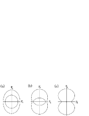
Figure 2: Fermi surfaces of the spectrum (11) for ${\bf q}//\hat{z}$. $p_{t}=\sqrt{p_{x}^{2}+p_{y}^{2}}$.   The outer (inner) closing line corresponds to $E_{-}(p)$ ($E_{+}(p)$). (a) for $M\geq q/2$; the minimum of $E_{-}(p)$ is at the origin. (b) for $M\leq q/2$; there are two minima at points $(p_{t},p_{z})=\left(0,\pm\sqrt{(q/2)^{2}-M^{2}}\right)$. (c) for $M\leq q/2$ and $\mu=q/2+M$; the minor Fermi sea vanishes.

In the density-wave state, all the energy levels below the chemical potential are occupied in the deformed spectrum. Accordingly the thermodynamic potential density at zero temperature becomes

$$\Omega_{\rm tot} = N_{f}N_{c}\int\frac{{\rm d}^{3}p}{(2\pi)^{3}}\sum_{s=\pm}\left[\left\{E_{s}(p)-\mu\right\}\theta\left(\mu-E_{s}(p)\right)-E_{s}(p)\right]+\frac{M^{2}}{4G}$$ (24)

$$\equiv \Omega_{\rm fer}+\Omega_{\rm vac}+\frac{M^{2}}{4G},$$

where $\Omega_{\rm fer}$ ($\Omega_{\rm vac}$) denotes the Fermi-sea (Dirac-sea) contribution. We can see that the finite wavenumber effect enters only through the deformation of the energy spectrum, and gives non-trivial contributions to the behaviour of the chiral condensation or the dynamical mass $M$. The energy gap between the two branches is generated by the dynamical mass which comes mainly from the Dirac sea, and the energy gain due to the density wave (to a finite $q$) comes essentially from the Fermi sea which is responsible for the finite baryon-number density, thus the DCDW is produced cooperatively by the Dirac and Fermi seas.

Since the NJL model is unrenormalizable, we need some regularization procedure to evaluate the negative-energy contribution $\Omega_{\rm vac}$. Because of the spectrum anisotropy we cannot apply the momentum cut-off regularization scheme. Instead we adopt the proper-time regularization (PTR) scheme sch . We show the result (the derivation is detailed in Appendix A),

$$\Omega_{\rm vac}=\frac{\gamma}{8\pi^{3/2}}\int_{1/\Lambda^{2}}^{\infty}\frac{{\rm d}\tau}{\tau^{5/2}}\int^{\infty}_{-\infty}\frac{{\rm d}p_{z}}{2\pi}\left[e^{-(\sqrt{p_{z}^{2}+m^{2}}+q/2)^{2}\tau}+e^{-(\sqrt{p_{z}^{2}+m^{2}}-q/2)^{2}\tau}\right]-\Omega_{{\rm ref}},$$ (25)

where $\Lambda$ is the cut-off parameter, and we subtracted an irrelevant constant $\Omega_{{\rm ref}}$ in the derivation. All the physical quantities should be taken to be smaller than the scale $\Lambda$ in the following calculations.

III.1 Phase transition at zero temperature

To investigate threshold density for formation of the density wave at $T=0$, we expand the potential (24) up to the second order in $q$, and examine the sign of its coefficient,

$$\Omega_{\rm tot} = \Omega_{\rm tot}^{0}+\frac{1}{2}(\beta_{\rm fer}+\beta_{\rm vac})q^{2}+O(q^{4})$$ (26)

$$\beta_{\rm fer} \equiv \frac{\partial^{2}\Omega_{\rm fer}}{\partial q^{2}}|_{q\rightarrow 0}=-N_{f}N_{c}\frac{M^{2}}{\pi^{2}}H(\mu/M)$$ (27)

$$\beta_{\rm vac} \equiv \frac{\partial^{2}\Omega_{\rm vac}}{\partial q^{2}}|_{q\rightarrow 0}=N_{f}N_{c}\frac{\Lambda^{2}}{2\pi^{2}}J(M^{2}/\Lambda^{2}),$$ (28)

where $J(x)=x\int_{x}^{\infty}{\rm d}\tau\exp(-\tau)/\tau$, and $H(x)={\rm ln}(x+\sqrt{x^{2}-1})$. The coefficient of the second-order term in $\Omega_{\rm fer}$ is always positive for finite dynamical mass $M\neq 0$, while the counterpart of $\Omega_{\rm vac}$ is negative, indicating that the Dirac sea is stiff against the formation of the density wave. In contrast, the Fermi sea favors it as mentioned in the previous section. The total coefficient, $\beta_{\rm tot}\equiv\beta_{\rm fer}+\beta_{\rm vac}$, depends on the dynamical mass and the chemical potential for fixed $\Lambda$, as shown in Fig. 3.

Figure 3: The dynamical-mass $M$ dependence of the coefficient $\beta_{tot}$ for various values of the chemical potential, (a) for $\mu/\Lambda=0.37-0.39$, (b) for $\mu/\Lambda=0.5-0.7$.

For larger values of the chemical potential in Fig. 3(b), $\beta_{{\rm tot}}$ becomes negative and reaches its maximum at a finite $M$. As for the small chemical potential $\mu/\Lambda<0.38$ in Fig. 3(a), $\beta_{\rm tot}$ never become negative for any value of $M$. It leads to a rough estimation of the critical coupling constant, $G\Lambda^{2}\simeq 4.63$, which is the value to occur the usual chiral condensation ($q=0$) at $\mu/\Lambda=0.38$ in the PTR scheme.

The magnitudes of $M$ and $q$ are obtained from the minimum of the potential (24) at $T=0$, and their values satisfy the stationary conditions, $\partial\Omega_{tot}/\partial M=\partial\Omega_{tot}/\partial q=0$.

Fig. 4 shows contours of $\Omega_{\rm tot}$ in $M$-$q$ plane for a given chemical potential, where the parameters are set as $G\Lambda^{2}=6$ and $\Lambda=850$ MeV, which are not far from those for the vacuum ($\mu=0$) kle .

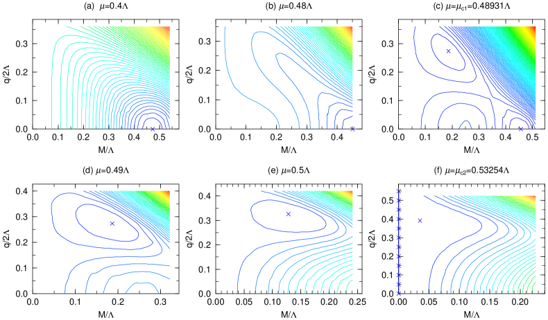
Figure 4: Contours of $\Omega_{tot}$ at $T=0$ are shown in $M$-$q$ plane as the chemical potential increases, (a) $\rightarrow$ (f). The cross in each figure denotes the absolute minimum.

The crossed points denote the absolute minima. There appear two critical chemical potentials $\mu=\mu_{c1},\mu_{c2}$: for the lower densities (Fig. 4(a)-(b)) the absolute minimum lies at the point $(M\neq 0,q=0)$ indicating a finite chiral condensation. At $\mu=\mu_{c1}$ (Fig. 4(c)) the potential has the two absolute minima at $(M\neq 0,q=0)$ and $(M\neq 0,q\neq 0)$, showing the first-order transition to the DCDW phase, which is stable for $\mu_{c1}<\mu<\mu_{c2}$ (Fig. 4(d)-(e)). At $\mu=\mu_{c2}$ (Fig. 4(f)) any point on the line $M=0$ and a point $(M\neq 0,q\neq 0)$ become minimum, and thereby the system undergoes the first-order transition to the chiral-symmetric phase which is stable for $\mu>\mu_{c2}$.

The Fig. 5 shows the behaviors of order-parameters $M$ and $q$ as functions of $\mu$ at $T=0$, where that of $M$ without the density wave is also shown for comparison.

Figure 5: Wavenumber $q$ and dynamical mass $M$ are plotted as functions of the chemical potential at $T=0$. Solid (dotted) line for $M$ with (without) the density wave, and dashed line for $q$.

It is found from the figure that the magnitude of $q$ becomes finite just before the critical point of the usual chiral transition, and DCDW survives at the finite range of $\mu$ ($\mu_{c1}\leq\mu\leq\mu_{c2}$) where the dynamical mass is reduced in comparison with that before the transition, and decreases with $\mu$. On the other hand, the wavenumber $q$ increases with $\mu$, but its value is smaller than twice the Fermi momentum $2k_{F}$($\simeq 2\mu$ for free quarks) due to the higher dimensional effect; the nesting of Fermi surfaces is incomplete in the present 3-D system. Actually, the ratio of the wavenumber and the Fermi momentum (at normal phase $q=M=0$) becomes $q/k_{F}=1.17-1.47$ for the baryon-number densities $\rho_{b}/\rho_{0}=3.62-5.30$ where DCDW develops. The baryon-number density is shown in Fig. 6 as a function of $\mu$ for the normal and the density wave cases. The jumps of the baryon-number density reflects the first-order transition.

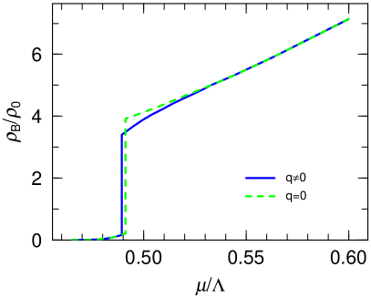
Figure 6: Baryon number density as a function of $\mu$. $\rho_{0}=0.16{\rm fm}^{-3}$: the normal nuclear density. Solid (dashed) line is for the finite $q$ ($q=0$).

In the DCDW phase, the relation $q/2>M$ is retained, and the Fermi surface looks like Fig. 2(b).

Here we show the coupling-strength dependence of the critical chemical potentials $\mu_{c1,c2}$ in Fig. 7, including the semi-empirical value, $G\Lambda^{2}=6.35$ ($\Lambda=660.37$ MeV), to reproduce the pion decay constant $f_{\pi}=93$ MeV and the constituent-quark mass $\simeq 330$ MeV, one third of the nucleon mass in the vacuum.

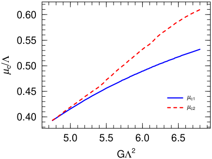
Figure 7: Critical chemical potentials $\mu_{c1,c2}$ are plotted as functions of the dimensionless coupling $G\Lambda^{2}$ at $T=0$. DCDW phase appears between $\mu_{c1}$ and $\mu_{c2}$. The critical coupling at $\mu_{c1}=\mu_{c2}$ is estimated to be $G\Lambda^{2}\simeq 4.72$.

The range of DCDW phase between $\mu_{c1}$ and $\mu_{c2}$ starts to open at $G\Lambda^{2}\simeq 4.72$, and broadens with increase of the coupling strength. It should be noted that the effective potential (24) can be scaled by the cut-off $\Lambda$ and thus the dimensionless coupling $G\Lambda^{2}$ becomes only one parameter to determine whether or not the phase transition itself occurs in the present model.

It should be kept in mind that the order of the transitions may depend on the parameter choice of $G$ and $\Lambda$, and may also on the regularization scheme.

III.2 Magnetic properties

Using the eigen spinors in eqs. (14)-(20), we can calculate various expectation values with respect to the DCDW state. For a operator, $\mathcal{O}$, which does not depend on the spatial coordinate, its expectation value becomes a simple form:

$$\langle\psi^{\dagger}(r)\mathcal{O}\psi(r)\rangle=\int\frac{{\rm d}^{3}p}{(2\pi)^{3}}\langle\tilde{\psi}^{\dagger}(p)~{}e^{i\tau_{3}\gamma_{5}{\bf q}\cdot{\bf r}/2}\mathcal{O}e^{-i\tau_{3}\gamma_{5}{\bf q}\cdot{\bf r}/2}~{}\tilde{\psi}(p)\rangle.$$ (29)

We can confirm that baryon-number density, $\mathcal{O}=1$, is still constant even in the density wave state: summation of quasi-particle state in momentum space,

$$\rho_{B}=\int\frac{{\rm d}^{3}p}{(2\pi)^{3}}\langle\tilde{\psi}^{\dagger}(p)\tilde{\psi}(p)\rangle=constant.$$ (30)

On the other hand, the spin expectation value, $\mathcal{O}=\gamma_{0}\gamma_{5}\gamma_{3}/2\equiv\Sigma_{z}$, vanishes in each flavor,

$$\langle\Sigma_{z}\rangle\equiv\frac{1}{2}\int\frac{{\rm d}^{3}p}{(2\pi)^{3}}\langle\tilde{\psi}^{\dagger}(p)\gamma_{0}\gamma_{5}\gamma_{3}\tilde{\psi}(p)\rangle=0,$$ (31)

because the stationary condition for the wavenumber $q$ is proportional to the expectation value:

$$0=\frac{\partial\Omega_{tot}(q,M)}{\partial q}\propto\langle\Sigma_{z}\rangle.$$ (32)

Here we show an interesting feature of DCDW: a spatial modulation of the anomalous magnetic moment. The Gordon decomposition of the gauge coupling term gives the magnetic interaction with external field $F^{\mu\nu}$ in the form, $g_{L}(e^{*}/2M)(\bar{\psi}\sigma_{\mu\nu}\psi)F^{\mu\nu}$, where $g_{L}$ is a form factor and $e^{*}$ an effective electric charge. The operator of the magnetic moment for the $z$ component is defined by $\mathcal{O}=\gamma_{0}\sigma_{12}$, which is not commuted to $\gamma_{5}$,

$$e^{i\tau_{3}\gamma_{5}{\bf q}\cdot{\bf r}/2}\gamma_{0}\sigma_{12}e^{-i\tau_{3}\gamma_{5}{\bf q}\cdot{\bf r}/2} = \gamma_{0}\sigma_{12}\cos({\bf q}\cdot{\bf r})-i\gamma_{3}\sin({\bf q}\cdot{\bf r}),$$ (33)

and then its expectation value is given by

$$\langle\bar{\psi}(r)\sigma_{12}\psi(r)\rangle = \langle\gamma_{0}\sigma_{12}\rangle\cos({\bf q}\cdot{\bf r})-i\langle\gamma_{3}\rangle\sin({\bf q}\cdot{\bf r}),$$ (34)

$$\mbox{where}~{}~{}\langle\gamma_{0}\sigma_{12}\rangle = \int\frac{{\rm d}^{3}p}{(2\pi)^{3}}\frac{2M}{\sqrt{M^{2}+p_{z}^{2}}}\left[n_{+}({{\bf p}})-n_{-}({{\bf p}})\right],$$ (35)

$$\langle\gamma_{3}\rangle = 0.$$ (36)

The function $n_{\pm}({\bf p})$ is the momentum distribution for the eigen state corresponding to $E_{\pm}({\bf p})$. The expectation value $\langle\gamma_{0}\sigma_{12}\rangle$ is proportional to an asymmetry of the momentum distribution in $n_{\pm}({\bf p})$. In DCDW phase, the asymmetry becomes finite as shown in Fig. 2, and thus the magnetic moment is spatially modulated with wavenumber $q$. The expectation value $\langle\gamma_{3}\rangle$ vanishes in each eigen spinor: $u^{\dagger}_{\pm}\gamma_{3}u_{\pm}=v^{\dagger}_{\pm}\gamma_{3}v_{\pm}=0$. We also confirmed that the other components of the magnetic moment, $\gamma_{0}\sigma_{23,13}$, vanished analytically after the integration in momentum space.

The equation (34) shows that the amplitude of the modulated magnetic moment depends on the dynamical mass, reflecting delay of chiral restoration due to the presence of DCDW. The magnetic order of DCDW should have some observable consequence of compact stars with quark cores. We estimate the magnitude of the amplitude (35) at $\rho_{B}/\rho_{0}=3\sim 4$: the tensor expectation value per quark is calculated to be $\langle\gamma_{0}\sigma_{12}\rangle/\langle\gamma_{0}\rangle=0.1\sim 0.3$. Thus a local magnetic flux $\Phi$ induced by DCDW,

$$\Phi=\left(\frac{2}{3}-\frac{1}{3}\right)\frac{e}{2m_{q}}\frac{\langle\gamma_{0}\sigma_{12}\rangle}{\langle\gamma_{0}\rangle}3\rho_{B},$$ (37)

amounts to $O(10^{16})$ Gauss, which is comparable with observed values in magnetars Mag1 . The flux strength on the star surface from the quark core might be smaller, since it is given by summation of the quark-magnetic moment (34) modulated rapidly with the wave length $q/2\pi\simeq O(10)$ fm, nevertheless, contributions from near the quark-core surface may remain without the cancellation.

III.3 Correlation functions

In this section, we consider scalar- and pseudoscalar-correlation functions, $\Pi_{\rm s,sp}(k)$, at the chirally restored phase, and discuss their relation with DCDW at $T=0$. The correlation functions depend on an external four-momentum $k=(k_{0},{\bf k})$, chemical potential, and also the effective quark mass for a given chemical potential. In the static limit $k_{0}\rightarrow 0$, the correlation functions have a physical correspondence to the static susceptibility functions for the spin- or charge-density wave kagoshima , while they have no primal singularity at $|{\bf k}|=2k_{F}$ reflecting the higher dimensionality. Note that the functions have a differential singularity at $k=2k_{F}$.

In general, a pole of the correlation function implies a second-order phase transition. As for the case of DCDW, the effective potential analysis in the previous section shows the first-order transtion. Nevertheless, as shown in Fig. 4(f), the potential barrier from DCDW to the normal phase at the critical point $\mu=\mu_{c2}$ is very small, and it is expected that the correlation function has some imformations of the transition point.

We evaluate effective interactions, $\Gamma_{\rm s,sp}(k)$, within the random phase approximation nam ; kle , which are related to the correlation functions, i.e., $2G\Pi_{\rm s,sp}(k)=\Gamma_{\rm s,sp}(k)\Pi_{\rm s,sp}^{0}(k)$:

$$i\Gamma_{\rm s,ps}(k) = \frac{2Gi}{1-2G\Pi_{\rm s,ps}^{0}(k)},$$ (38)

where $\Pi_{\rm s,ps}^{0}(k)$ is the polarization function in medium, which has form at the static and chiral limits (see Appendix C):

$$\Pi_{\rm s}^{0}(|{\bf k}|)=\Pi_{\rm ps}^{0}(|{\bf k}|) = \frac{N_{f}N_{c}}{4\pi^{2}}(\Lambda^{2}-2k_{F}^{2})-2N_{f}N_{c}i{\bf k}^{2}I({\bf k}^{2})|_{M\rightarrow 0}$$ (39)

$$+ \frac{N_{f}N_{c}|{\bf k}|}{4\pi^{2}}\left[k_{F}\log\left(\frac{2k_{F}+|{\bf k}|}{2k_{F}-|{\bf k}|}\right)+\frac{|{\bf k}|}{2}\log\left\{\frac{\left(2k_{F}+|{\bf k}|\right)\left(2k_{F}-|{\bf k}|\right)}{|{\bf k}|^{2}}\right\}\right].$$

Inverse of the correlation function in the chiral limit corresponds to the coefficient of $M^{2}$ of the effective potential,

$$\Omega_{tot}=\Omega_{tot}|_{M\rightarrow 0}+\frac{1}{2}\Gamma_{\rm ps}^{-1}(q)|_{M\rightarrow 0}M^{2}+O(M^{4}).$$ (40)

From behaviors of the function $\Gamma_{\rm ps}(|{\bf k}|)^{-1}$ shown in Fig. 8(a), it is found that the function takes the lowest value at a finite external momentum ($|{\bf k}|\simeq 1.5k_{F}$), and thus a finite wavenumber $q$ gives the lower potential energy in eq. (40). Assuming the second-order transition, the critical density $\mu_{t}$ and wavenumber $|{\bf k}_{t}|$ are determined from a following simultaneous equation:

$$\Gamma_{\rm sp}(|{\bf k}|;\mu)^{-1}=0,~{}~{}\mbox{and}~{}~{}\frac{\partial\Gamma_{\rm sp}(|{\bf k}|;\mu)^{-1}}{\partial|{\bf k}|}=0.$$ (41)

A numerical calculation in the chiral limit gives $\mu_{t}(=k_{F})=0.5320\Lambda$ and $|{\bf k}_{t}|=1.498k_{F}$, which almost coincide with the correct result $\mu_{c2}=0.53254\Lambda$ and $q=1.469k_{F}$ (where $k_{F}\equiv\sqrt{\mu_{c2}^{2}-M^{2}}$; $M=0.034\Lambda$) from the effective potential analysis. A complex structure of the effective potential makes a little difference between $|{\bf k}_{t}|$ and $q$ at $\mu=\mu_{c2}$.

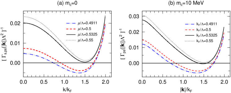
Figure 8: Function, $1/\Gamma_{\rm ps}(|{\bf k}|)$, is plotted for various values of $\mu$, $\mu/\Lambda=0.4911,0.5,0.53254(=\mu_{c2})$, and $0.55$, for $m_{c}=0$ (a) and $m_{c}=10$ MeV (b). In the case of $\mu/\Lambda\geq 0.4911$, the mass-gap equation has a extremum solution $M=0$.

The above argument might also be available even for the case of a finite current-quark mass, $m_{c}\simeq 10$MeV: the effective potential for a small current-quark mass ($m_{c}<<\mu$) is approximated to

$$\Omega_{tot}\simeq\Omega_{tot}|_{M\rightarrow m_{c}}+\frac{1}{2}\Gamma_{\rm ps}^{-1}(q)|_{M\rightarrow m_{c}}(M-m_{c})^{2}+O[(M-m_{c})^{4}].$$ (42)

The Fig. 8(b) shows that behaviors of the coefficient function has little shift from that of the chiral limit, and thus suggests a DCDW transition with a small current-quark mass as in the chiral limit.

III.4 Phase diagram on the $\mu$-$T$ plane

To complete a phase diagram we derive the thermodynamic potential at finite temperature in the Matsubara formalism. The partition function for the mean-field Hamiltonian is given by

$$Z_{\beta}=\int{\it D}\bar{\psi}{\it D}\psi\exp\int_{0}^{\beta}{\rm d}\tau\int{\rm d}^{3}r~{}\left\{\bar{\psi}\left[i\tilde{\partial}+M\exp\left(i\gamma_{5}{\bf q}\cdot{\bf r}\right)-\gamma_{0}\mu\right]\psi-\frac{M^{2}}{4G}\right\},$$ (43)

where $\beta=1/T$, and $\tilde{\partial}\equiv-\gamma_{0}\partial_{\tau}+i{\bf\gamma}\nabla$. Taking the Fourier transform of the spinor with the Matsubara frequency $\omega_{n}$, the partition function becomes

$$\psi({\bf r},-i\tau) = e^{-i\tau_{3}\gamma_{5}{\bf q}\cdot{\bf r}/2}~{}T\sum_{n}\int\frac{{\rm d}^{3}{\bf k}}{(2\pi)^{3}}e^{i\omega_{n}\tau+i{\bf k}\cdot{\bf r}}\tilde{\psi}({\bf k},n),$$

$$Z_{\beta} = \prod_{{\bf k},n,s=\pm}\left\{(i\omega_{n}+\mu)^{2}-E_{s}^{2}({\bf k})\right\}^{N_{f}N_{c}}\times\exp\left\{-\left(\frac{M^{2}}{4G}\right)V\beta\right\},$$ (44)

where $V$ is volume of the system. Thus the thermodynamic potential $\Omega_{\beta}$ per unit volume is obtained,

$$\Omega_{\beta}(q,M) = -T\log{Z_{\beta}(q,M)}/V$$ (45)

$$= -N_{f}N_{c}\int\frac{{\rm d}^{3}{\bf k}}{(2\pi)^{3}}\sum_{s=\pm}\left\{T\log{\left[e^{-\beta\left(E_{s}({\bf k})-\mu\right)}+1\right]\left[e^{-\beta\left(E_{s}({\bf k})+\mu\right)}+1\right]}+E_{s}({\bf k})\right\}+\frac{M^{2}}{4G}$$

where we have utilized a contour-integral technique for the frequency sum to get the final form.

From the absolute minimum of the thermodynamic potential (45), it is found that the order parameters at $T\neq 0$ behave similarly to those at $T=0$ as a function of $\mu$, while the chemical-potential range of DCDW, $\mu_{c1}(T)\leq\mu\leq\mu_{c2}(T)$, gets smaller as $T$ increases. The Fig. 9 shows the order parameters at finite temperature.

Figure 9: The wavenumber $q$ and the dynamical mass $M$ are plotted as a function of $\mu$ at finite temperature. The solid (dashed) line corresponds to $q$ ($M$) at $T/\Lambda=0.02$ (thick lines), $0.03$ (thin lines).

The discontinuities of the order parameters reflect the two absolute minima at the critical chemical potential $\mu_{c1,2}$, and it indicates a first-order transition. Thus the region of DCDW in the $\mu$-$T$ phase diagram is surrounded by the first-order transition lines.

We show the resultant phase diagram in Fig. 10, where the usual chiral-transition line is also given for reference.

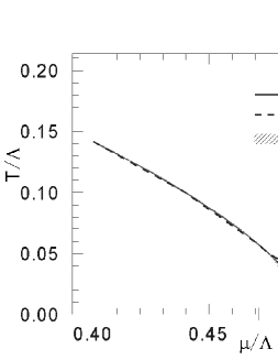
Figure 10: A phase diagram obtained from the thermodynamic potential eq. (45). The solid (dashed) line shows the chiral-transition line without (with) the DCDW. The shaded area shows the DCDW phase.

Comparing phase diagrams with and without $q$, we find that the DCDW phase emerges in the area (shaded area in Fig. 10) which lies just outside the boundary of the ordinary chiral transition. We thus conclude that DCDW is induced by finite-density contributions, and has the effect to extend the chiral-condensed phase ($M\neq 0$) to a low temperature ($T_{c}\sim 50$MeV) and high density region. The above results suggests that QCD at finite density involves rich and nontrivial phase structures, as well as color superconducting phases.

IV Summary and outlooks

We have discussed a possibility of the dual chiral-density wave in moderate-density quark matter within the mean-field approximation, employing 2-flavor and 3-color NJL model. The mechanism of the density wave is quite similar to the spin density wave in 3-D electron systems; the total-energy gain comes from the Fermi-sea contribution in the deformed spectrum, while its amplitude has the different origin corresponding to the chiral condensation from the Dirac-sea effect.

In this paper, we have considered only the direct channels (Hartree terms) of the interaction. If the exchange channels (Fock term) are involved, there appear additional interaction channels by way of the Fierz transformation kle . In particular, self-energies in axial-vector and tensor channels related to a ferromagnetism nak ; mar might affect the density wave through nontrivial correlations among them. Interactions in the p-p channels are also obtained by the Fierz transformation, and their strength is smaller than that of the direct channels by the factor of $O(1/N_{c})$. Because the Cooper instability is independent on the strength of the interaction, it is interesting to investigate the interplay among the density wave, superconductivity der1 ; der2 ; Ohwa , and the other ordered phases, e.g., chiral-density waves mixing isospins which may cause a charge-density wave due to difference of electric charges of u- and d-quarks, as future studies.

Finally, it is worth mentioning about correlation functions (fluctuation modes) on the density-wave phase, which give the excitation spectrum, and are important for the dynamical description of the phase. In particular, Nambu-Goldstone modes are essential degrees of freedom for low-energy phenomena, and may bring some observable consequences, e.g., slowing down of star cooling through enhancement of specific heat due to fluctuations of such low-energy modes.

Acknowledgements

Authors thank T. Maruyama, K. Nawa, and H. Yabu for discussions and comments. The present research is partially supported by the Grant-in-Aid for the 21st century COE “Center for Diversity and Universality in Physics” of the Ministry of Education, Culture, Sports, Science and Technology, and by the Japanese Grant-in-Aid for Scientific Research Fund of the Ministry of Education, Culture, Sports, Science and Technology (11640272, 13640282).

Appendix A Regularization of $\Omega_{\rm vac}$

We regularize the Dirac-sea contributions to the potential, $\Omega_{\rm vac}$, by applying the schwinger’s proper-time method. $\Omega_{\rm vac}$ can be described in the form of the one-loop order contribution,

$$\Delta\Omega=\Omega_{\rm vav}(q,M)-\Omega_{\rm N} = -\int_{C}\frac{{\rm d}^{4}k}{i(2\pi)^{4}}\sum_{s=\pm}\log\frac{D_{s}}{D_{N}}$$ (46)

with $$D_{\pm}=k_{0}^{2}-E_{\pm}^{2}({\bf k})~{}~{}\mbox{and}~{}~{}D_{N}=k_{0}^{2}-{\bf k}^{2}-m^{2},$$ (47)

where $\Omega_{\rm N}$ is the normal vacuum contribution. Using the identity for $G\in{\bf R}$

$$(G+i\eta)^{-1}=-i\int_{0}^{\infty}{\rm d}s~{}e^{i(G+i\eta)s},$$ (48)

we find

$$\log\frac{D_{\pm}+i\eta}{D_{N}+i\eta}=-\int_{0}^{\infty}\frac{{\rm d}s}{s}\left(e^{i(D_{\pm}+i\eta)s}-e^{i(D_{\rm N}+i\eta)s}\right).$$ (49)

By way of the Wick rotation which is done simultaneously for $k_{0}$ integration of $\Omega_{\rm vac}$ and $\Omega_{\rm N}$,

$$\Delta\Omega_{\pm} = \int_{C}\frac{{\rm d}^{4}k}{i(2\pi)^{4}}\int_{0}^{\infty}\frac{{\rm d}s}{s}\left(e^{iD_{\pm}s}-e^{iD_{0}s}\right)$$

$$= \int_{-\infty}^{\infty}\frac{{\rm d}^{4}k_{E}}{(2\pi)^{4}}\int_{0}^{\infty}\frac{{\rm d}s}{s}\left[\exp i\{-k_{E}^{2}-k_{t}^{2}-(\sqrt{k_{z}^{2}+M^{2}}\pm q/2)^{2}\}s\right.$$

$$~{}~{}~{}~{}~{}~{}~{}~{}~{}~{}~{}~{}~{}~{}~{}~{}~{}~{}~{}~{}~{}~{}~{}~{}~{}~{}~{}~{}~{}~{}~{}~{}~{}-\left.\exp i\{-k_{E}^{2}-k_{t}^{2}-k_{z}^{2}-m^{2}\}s\right]$$

$$= \int_{-\infty}^{\infty}\frac{{\rm d}^{4}k_{E}}{(2\pi)^{4}}\int_{0}^{\infty}\frac{{\rm d}\tau}{\tau}\left[\exp\{-k_{E}^{2}-k_{t}^{2}-(\sqrt{k_{z}^{2}+M^{2}}\pm q/2)^{2}\}\tau\right.$$

$$~{}~{}~{}~{}~{}~{}~{}~{}~{}~{}~{}~{}~{}~{}~{}~{}~{}~{}~{}~{}~{}~{}~{}~{}~{}~{}~{}~{}~{}~{}~{}~{}~{}-\left.\exp\{-k_{E}^{2}-k_{t}^{2}-k_{z}^{2}-m^{2}\}\tau\right]$$

$$= \frac{1}{8\pi^{3/2}}\int_{0}^{\infty}\frac{{\rm d}k_{z}}{2\pi}\int_{0}^{\infty}\frac{{\rm d}\tau}{\tau^{5/2}}\left[\exp\{-(\sqrt{k_{z}^{2}+M^{2}}\pm q/2)^{2}\tau\}-\exp\{-(k_{z}^{2}+m^{2})\tau\}\right]$$

The above integration of $\tau$ has singular at $\tau=0$ and thus not well defined. The proper-time regularization is to replace the lower limit of $\tau$ by the cutoff $1/\Lambda^{2}$,

$$\int_{0}^{\infty}{\rm d}\tau\rightarrow\int_{1/\Lambda^{2}}^{\infty}{\rm d}\tau,$$ (51)

the $\Lambda$ corresponds to a momentum cutoff.

Eventually we obtain the regularized potential from the Dirac sea,

$$\Delta\Omega = \Delta\Omega_{+}+\Delta\Omega_{-}$$ (52)

$$= \frac{1}{8\pi^{3/2}}\int_{0}^{\infty}\frac{{\rm d}k_{z}}{2\pi}\int_{1/\Lambda^{2}}^{\infty}\frac{{\rm d}\tau}{\tau^{5/2}}\left[\exp\{-(\sqrt{k_{z}^{2}+M^{2}}+q/2)^{2}\tau\}+\exp\{-(\sqrt{k_{z}^{2}+M^{2}}-q/2)^{2}\tau\}\right.$$

$$~{}~{}~{}~{}~{}~{}~{}~{}~{}~{}~{}~{}~{}~{}~{}~{}~{}~{}~{}~{}~{}~{}~{}~{}~{}~{}~{}~{}~{}~{}~{}~{}~{}~{}~{}~{}~{}~{}~{}~{}~{}~{}~{}~{}\left.-2\exp\{-(k_{z}^{2}+m^{2})\tau\}\right].$$

The normal vacuum contribution $\Omega_{N}$ has an explicit form,

$$\Omega_{N} = N_{c}N_{f}\frac{1}{8\pi^{2}}\int_{1/\Lambda^{2}}^{\infty}\frac{{\rm d}\tau}{\tau^{3}}e^{-m^{2}\tau}$$ (53)

$$= N_{c}N_{f}\frac{\Lambda^{4}}{16\pi^{2}}\left\{(-\tilde{m}^{2}+1)e^{-\tilde{m}^{2}}+\tilde{m}^{4}\Gamma(0,\tilde{m}^{2})\right\},$$

where $\tilde{m}=m/\Lambda$ and $\Gamma(a,z)=\int_{z}^{\infty}{\rm d}\tau\tau^{a-1}\exp(-\tau)$ is the incomplete gamma function.

Appendix B Fock exchange contributions

We briefly examine how the Fock exchange terms of the NJL interaction affect DCDW. After the Fierz transformation, one can find the exchange interaction terms, discarding color-octet contributions kle :

$$\mathcal{F}\left[\left(\bar{\psi}\psi\right)^{2}+\left(\bar{\psi}i\gamma_{5}{\bf\tau}\psi\right)^{2}\right] = \frac{1}{8N_{c}}\left[2\left(\bar{\psi}\psi\right)^{2}+2\left(\bar{\psi}i\gamma_{5}{\bf\tau}\psi\right)^{2}-2\left(\bar{\psi}{\bf\tau}\psi\right)^{2}-2\left(\bar{\psi}i\gamma_{5}\psi\right)^{2}\right.$$ (54)

$$-\left.4\left(\bar{\psi}\gamma_{\mu}\psi\right)^{2}-4\left(\bar{\psi}i\gamma_{5}\gamma_{\mu}\psi\right)^{2}+\left(\bar{\psi}\sigma_{\mu\nu}\psi\right)^{2}-\left(\bar{\psi}\sigma_{\mu\nu}{\bf\tau}\psi\right)^{2}\right]$$

The overall factor $1/8N_{c}$ indicates that the exchange terms are less relevant in comparison with the direct terms.

The first two terms come to be added to the Hartree terms, and contribute to DCDW through changing the effective interaction in these channels by a factor.

The third and fourth terms have opposite sign of interactions, and thereby they can not gain condensation energies.

The fifth one has an expectation value in its temporal term, which corresponds to the baryon number density, $\langle\psi^{\dagger}\psi\rangle\neq 0$, and is renormalized into the chemical potential hatsu ; asa . Thus it might not change DCDW qualitatively, except for changing value of a bare chemical potential for a fixed baryon number density. The other spatial terms vanish self-consistently in the present formalism nak .

The sixth term, the axial-vector interaction, seems to contribute DCDW because the Weinberg transformation leaves it unchanged, but scalar and pseudo-scalar terms for DCDW changed to an another axial-vector mean-field with isospin $\tau_{3}$. However, it is found that this term does not affect DCDW by itself: the Hartree-Fock free-energy with both the axial-vector mean-field $V_{A}$ and DCDW (the wavenumber $q$) is given, after the Weinberg transformation, by

$${\cal H}_{HF} = \int\bar{\psi}\left[{\bf p}^{2}+M^{2}+\gamma_{3}\gamma_{5}\left(V_{A}+\tau_{3}q/2\right)\right]\psi+\frac{M^{2}}{4G_{S}}+\frac{V_{A}^{2}}{4G_{A}},$$ (55)

$$= \int\bar{\psi}_{u}\left[{\bf p}^{2}+M^{2}+\gamma_{3}\gamma_{5}A\right]\psi_{u}+\int\bar{\psi}_{d}\left[{\bf p}^{2}+M^{2}+\gamma_{3}\gamma_{5}B\right]\psi_{d}+\frac{M^{2}}{4G_{S}}+\frac{(A+B)^{2}}{16G_{A}},$$

$$A = V_{A}+q/2,~{}\mbox{and}~{}B=V_{A}-q/2,$$

where $\psi_{u,d}$ are spinors of u,d-quark, and $G_{S,A}$ are reduced coupling constants in scalar and axial-vector channels. The equation (55) shows that the minimum of the effective potential is always given by $A+B=2V_{A}=0$ because the first two terms have the same structure in their energy spectrum with respect to $A,B$ independently of the sign of $A,B$, and implies, therefore, that the expectation value of the axial-vector channel vanishes.

The last two terms, the tensor interactions, might give a non trivial contribution to DCDW through an feedback effect of the nonzero expectation value of the tensor operator, $\langle\gamma_{0}\sigma_{12}\rangle$, see eq. (34), although their interaction strengths are small by the factor $1/8N_{c}$. This problem is left for a future study.

Appendix C Scalar and pseudo-scalar scattering amplitudes

Following Nambu nam , we consider the quark-quark scattering matrix generated by the chain diagram in the pseudo-scalar channel. Then the polarization function, $-i\Pi_{\rm ps}^{0}$, is given by

$$-i\Pi_{\rm ps}^{0}(k^{2})=-\int\frac{{\rm d}^{4}p}{(2\pi)^{4}}{\rm tr}\left[i\gamma_{5}\tau_{3}iS(p+\frac{1}{2}k)i\gamma_{5}\tau_{3}iS(p-\frac{1}{2}k)\right],$$ (56)

with the quark propagator in medium,

$$S(p) = \frac{1}{/{\!\!\!}{p}-m}+i\frac{\pi}{E_{p}}(/{\!\!\!}{p}+m)\theta(\mu-E_{p})\delta(p_{0}-E_{p})$$ (57)

$$\equiv (/{\!\!\!}{p}+m)\tilde{S}(p)=(/{\!\!\!}{p}+m)\left[\tilde{S}_{F}(p)+\tilde{S}_{D}(p)\right].$$

Then the scattering matrix $M_{33}^{\rm ps}$ can be written in the form,

$$iM_{33}^{\rm ps}(k^{2})=(i\gamma_{5})\tau_{3}\left[\frac{2iG}{1-2G\Pi^{0}_{\rm ps}(k^{2})}\right](i\gamma_{5})\tau_{3}.$$ (58)

There are three kinds of contributions to $\Pi_{\rm ps}^{0}(k^{2})$,

$$\Pi_{\rm ps}^{0}(k^{2})=\Pi_{\rm ps}^{FF}(k^{2})+\Pi_{\rm ps}^{DD}(k^{2})+2\Pi_{\rm ps}^{DF}(k^{2})$$ (59)

with

$$-i\Pi_{\rm ps}^{ij}(k^{2})=-4N_{f}N_{c}\int\frac{{\rm d}^{4}p}{(2\pi)^{4}}\left(-p^{2}+m^{2}+\frac{1}{4}k^{2}\right){\tilde{S}}_{i}\left(p+\frac{1}{2}k\right){\tilde{S}}_{j}\left(p-\frac{1}{2}k\right).$$ (60)

First, we consider the vacuum contribution,

$$-i\Pi_{\rm ps}^{FF}(k^{2}) = 2N_{f}N_{c}\int\frac{{\rm d}^{4}p}{(2\pi)^{4}}\left[\frac{1}{(p+\frac{1}{2}k)^{2}-m^{2}}+\frac{1}{(p-\frac{1}{2}k)^{2}-m^{2}}\right]$$ (61)

$$-2N_{f}N_{c}k^{2}\int\frac{{\rm d}^{4}p}{(2\pi)^{4}}\frac{1}{[(p+\frac{1}{2}k)^{2}-m^{2}][(p-\frac{1}{2}k)^{2}-m^{2}]}.$$

The integrals in the first term is easily evaluated to get

$$\int\frac{{\rm d}^{4}p}{(2\pi)^{4}}\frac{1}{(p\pm\frac{1}{2}k)^{2}-m^{2}}=-\frac{i}{16\pi^{2}}\int\frac{{\rm d}\tau}{\tau^{2}}e^{-m^{2}\tau},$$ (62)

in the proper-time representation. The integral in the second term is denoted by $I(k^{2})$,

$$I(k^{2})=\int\frac{{\rm d}^{4}p}{(2\pi)^{4}}\frac{1}{[(p+\frac{1}{2}k)^{2}-m^{2}][(p-\frac{1}{2}k)^{2}-m^{2}]}.$$ (63)

Using the Feynman’s trick,

$$I(k^{2}) = \int_{0}^{1}{\rm d}t\int\frac{{\rm d}^{4}p}{(2\pi)^{4}}\frac{1}{[p^{2}-m^{2}+(k^{2}+2pk)t]^{2}}$$ (64)

$$= \int_{0}^{1}{\rm d}t\int\frac{{\rm d}^{4}p}{(2\pi)^{4}}\frac{\partial}{\partial m^{2}}\frac{1}{p^{2}-m^{2}+k^{2}t(1-t)},$$

and introducing the proper-time $\tau$, we find

$$I(k^{2})=\frac{i}{16\pi^{2}}\int_{0}^{1}dt\int_{0}^{\infty}\frac{{\rm d}\tau}{\tau}e^{-(m^{2}-k^{2}t(1-t))\tau}.$$ (65)

The vacuum contribution is summarized as follows:

$$-i\Pi_{\rm ps}^{FF}(k^{2})=-\frac{iN_{f}N_{c}}{4\pi^{2}}\int\frac{{\rm d}\tau}{\tau^{2}}e^{-m^{2}\tau}+\frac{iN_{f}N_{c}}{8\pi^{2}}k^{2}\int_{0}^{1}{\rm d}t\int_{0}^{\infty}\frac{{\rm d}\tau}{\tau}e^{-(m^{2}-k^{2}t(1-t))\tau}.$$ (66)

Secondly, let us consider $\Pi_{\rm ps}^{DF}(k^{2})$,

$$-i\Pi_{\rm ps}^{DF}(k^{2}) = -4N_{f}N_{c}\int\frac{{\rm d}^{3}p}{(2\pi)^{4}}\left[-\left(\frac{1}{2}k_{0}+E_{{\bf p}-\frac{1}{2}{\bf k}}\right)^{2}+{\bf p}^{2}+m^{2}+\frac{1}{4}k^{2}\right]$$ (67)

$$\times \frac{1}{\left(k_{0}+E_{{\bf p}-\frac{1}{2}{\bf k}}\right)^{2}-\left({\bf p}+\frac{1}{2}{\bf k}\right)^{2}-m^{2}}\frac{i\pi}{E_{{\bf p}-\frac{1}{2}{\bf k}}}\theta(\mu-E_{{\bf p}-\frac{1}{2}{\bf k}}).$$

Taking the static limit $k_{0}\rightarrow 0$, we have

$$-i\Pi_{\rm ps}^{DF}(|\bf k|) \rightarrow 2N_{f}N_{c}i\int\frac{{\rm d}^{3}p}{(2\pi)^{3}}\frac{{\bf p}\cdot{\bf k}}{2{\bf p}\cdot{\bf k}+{\bf k}^{2}}\frac{1}{E_{p}}\theta(\mu-E_{p})$$ (68)

$$= 2N_{f}N_{c}i\int_{-1}^{1}{\rm d}x\int\frac{p^{2}{\rm d}p}{(2\pi)^{2}}\left[1-\frac{|\bf k|}{2px+|\bf k|}\right]\frac{1}{E_{p}}\theta(\mu-E_{p})$$

$$= i\frac{N_{f}N_{c}}{4\pi^{2}}\left[p_{F}\mu-m^{2}\ln\left(\frac{p_{F}+\mu}{m}\right)-\frac{|\bf k|}{2}\int_{0}^{p_{F}}p{\rm d}p\ln\left|\frac{2p+|\bf k|}{2p-|\bf k|}\right|\frac{1}{E_{p}}\right]$$

$$+\frac{N_{f}N_{c}|\bf k|}{8\pi}\left[\mu-\left(m^{2}+\frac{|\bf k|^{2}}{4}\right)^{1/2}\right].$$

The integral over the Fermi sea can be analytically performed, but we do not write it down here because of its complexity.

Finally, we calculate $\Pi_{\rm ps}^{DD}(k^{2})$,

$$-i\Pi_{\rm ps}^{DD}(k^{2}) = -\int\frac{{\rm d}^{4}p}{(2\pi)^{4}}4N_{f}N_{c}\left(-p^{2}+m^{2}+\frac{1}{4}k^{2}\right){\tilde{S}_{D}\left(p+\frac{1}{2}k\right)}{\tilde{S}_{D}\left(p-\frac{1}{2}k\right)}$$ (69)

$$= -\int\frac{{\rm d}^{3}p}{(2\pi)^{4}}4N_{f}N_{c}\left[-\left(\frac{1}{2}k_{0}+E_{p}\right)^{2}+\left({\bf p}+\frac{1}{2}{\bf k}\right)^{2}+m^{2}+\frac{1}{4}k^{2}\right]$$

$$\times \frac{i\pi}{E_{{\bf p}+{\bf k}}}\theta(\mu-E_{{\bf p}+{\bf k}})\delta(k_{0}+E_{\bf p}-E_{{\bf p}+{\bf k}})\theta(\mu-E_{\bf p}).$$

In the static limit $k_{0}\rightarrow 0$,

$$-i\Pi_{\rm ps}^{DD}(|{\bf k}|)\rightarrow-N_{f}N_{c}\frac{|{\bf k}|}{4\pi}\left[\mu-\left(m^{2}+\frac{{\bf k}^{2}}{4}\right)^{1/2}\right],$$ (70)

which exactly cancels the imaginary part arising from $\Pi_{\rm ps}^{DF}(|{\bf k}|)$.

Collecting them together, we have the denominator of the scattering amplitude in the static limit,

$$1-2G\Pi_{\rm ps}^{0}(|{\bf k}|) = 1-2G(\Pi_{\rm ps}^{FF}(|{\bf k}|)+2\Pi_{\rm ps}^{FD}(|{\bf k}|)+\Pi_{\rm ps}^{DD}(|{\bf k}|))$$ (71)

$$= 1-2G\frac{N_{f}N_{c}}{4\pi^{2}}\int\frac{{\rm d}\tau}{\tau^{2}}e^{-m^{2}\tau}-4GiN_{f}N_{c}{\bf k}^{2}I({\bf k}^{2})$$

$$+ G\frac{N_{f}N_{c}}{\pi^{2}}\left[p_{F}\mu-m^{2}\ln\left(\frac{p_{F}+\mu}{m}\right)-\frac{|{\bf k}|}{2}\int_{0}^{p_{F}}p{\rm d}p\ln\left|\frac{2p+|{\bf k}|}{2p-|{\bf k}|}\right|\frac{1}{E_{p}}\right].$$

On the other hand, the gap equation in this case reads

$$m=m_{c}+\frac{1}{2\pi^{2}}GN_{f}N_{c}m\int\frac{{\rm d}\tau}{\tau^{2}}e^{-m^{2}\tau}-G\frac{N_{f}N_{c}}{\pi^{2}}m\left[p_{F}\mu-m^{2}\ln\left(\frac{p_{F}+\mu}{m}\right)\right].$$ (72)

Thus, we find at a stationary point (at a solution of the gap equation),

$$1-2G\Pi_{\rm ps}^{0}(|{\bf k}|) = \frac{m_{c}}{m}-4GiN_{f}N_{c}{\bf k}^{2}I({\bf k}^{2})-G\frac{N_{f}N_{c}}{2\pi^{2}}|{\bf k}|\int_{0}^{p_{F}}p{\rm d}p\ln\left|\frac{2p+|{\bf k}|}{2p-|{\bf k}|}\right|\frac{1}{E_{p}}.$$ (73)

In the similar way, the scattering amplitude of scalar channel is given by

$$1-2G\Pi_{\rm s}^{0}(|{\bf k}|) = 1-2G\frac{N_{f}N_{c}}{4\pi^{2}}\int\frac{{\rm d}\tau}{\tau^{2}}e^{-m^{2}\tau}-4GiN_{f}N_{c}({\bf k}^{2}+4m^{2})I({\bf k}^{2})$$ (74)

$$+ G\frac{N_{f}N_{c}}{\pi^{2}}\left[p_{F}\mu-m^{2}\ln\left(\frac{p_{F}+\mu}{m}\right)-\frac{{\bf k}^{2}+2m^{2}}{2|{\bf k}|}\int_{0}^{p_{F}}p{\rm d}p\ln\left|\frac{2p+|{\bf k}|}{2p-|{\bf k}|}\right|\frac{1}{E_{p}}\right]$$

$$+ 2GN_{f}N_{c}i\frac{m^{2}}{2\pi|{\bf k}|}\left[\mu-\sqrt{m^{2}+{\bf k}^{2}/4}\right]\theta\left(2k_{F}-|{\bf k}|\right).$$

References

-
(1)
D. Bailin and A. Love, Phys. Rep. 107(1984) 325.
For a recent review, M. Alford, Ann. Rev. Nucl. Part. Sci. 51 (2001) 131. - (2) M. Alford, K. Rajagopal, and F. Wilczek, Phys. Lett. B442 (1998) 247.
- (3) R. Rapp, T.Schäfer, E. V. Shuryak, and M. Velkovsky, Phys. Rev. Lett. 88 (1998) 53.
-
(4)
J. Madsen, Phys. Rev. Lett. 85 (2000) 10,
M. Prakash, Nucl. Phys. A698 (2002) 440,
M. Prakash, J. M. Lattimer, A. W. Steiner, D. Page, Nucl. Phys. A715 (2003) 835. - (5) T. Tatsumi, Phys. Lett. B489 (2000) 280.
- (6) E. Nakano, T. Maruyama and T. Tatsumi, Phys. Rev. D68 (2003) 105001.
- (7) A. Niégawa, hep-ph/0404252.
- (8) E. Shuster and D. T. Son, Nucl. Phys. B573 (2000) 434.
-
(9)
B.-Y. Park, M.Rho, A.Wirzba and I.Zahed, Phys. Rev. D62 (2000) 034015.
R. Rapp, E.Shuryak and I. Zahed, Phys. Rev. D63 (2001) 034008. - (10) D.V. Deryagin, D. Yu. Grigoriev and V.A. Rubakov, Int. J. Mod. Phys. A7 (1992) 659.
- (11) S. Kagoshima, H. Nagasawa, and T. Sambongi, One Dimensional Conductors, Springer series in solid-state sciences, Vol. 72 (Springer-Verlag, Berlin, 1988); L. P. Gor’kov and G. Grüner, Charge Density waves in Solids, MODERN PROBLEMS IN CONDENSED MATTER SCIENCES. VOL. 25 (AMSTERDAM: North-Holland, 1989).
- (12) R. E. Peierls, Quantum Theory of Solids (Oxford University Press, London, 1955).
- (13) G. Grüner, Rev. Mod. Phys. 60 4 (1988) .
- (14) A.W. Overhauser, Phys. Rev. Lett.4 462 (1960); Phys. Rev. 128 1437 (1962).
- (15) G. Grüner, Rev. Mod. Phys. 66 1 (1994).
- (16) T. Tatsumi and E. Nakano, hep-ph/0408294.
- (17) Y. Nambu and G. Jona-Lasinio, Phys. Rev. 122 345 (1961); 124 246 (1961).
- (18) S. Weinberg, The quantum theory of field II (Cambridge, 1996).
- (19) S.P. Klevansky, Rev. Mod. Phys. 64 649 (1992).
-
(20)
F. Dautry and E.M. Nyman, Nucl. Phys. 319 323 (1979).
K. Takahashi and T. Tatsumi, Phys. Rev. C63 015205 (2000); Prog. Theor. Phys. 105 437 (2001).
M. Kutschera, W. Broniowski and A. Kotlorz, Nucl. Phys. A516 566 (1990).
M. Sadzikowski and W. Broniowski, Phys. Lett. 488 63 (2000). - (21) T Schaefer, Phys.Rev. D62 094007 (2000).
- (22) J. Schwinger, Phys. Rev. 92 664 (1951).
- (23) M. Asakawa and K. Yazaki, Nucl. Phys. A 504 668 (1989).
- (24) T. Hatsuda and T. Kunihiro, Phys. Rep. 247 221 (1994).
- (25) T. Maruyama and T. Tatsumi, Nucl. Phys. A693 710 (2001).
- (26) C. Kouveliotou et al., Nature (London) 393, 235 (1998); K. Hurley et al., Astrophys. J. Lett. 510, L111 (1999).
- (27) K. Ohwa, Phys. Rev. D65, 085040 (2002).