Hadronic decays of the tau lepton : Theoretical overview

Abstract

Exclusive hadronic decays of the tau lepton provide an excellent framework to study the hadronization of QCD currents in a non-perturbative energy region populated by many resonances. I give a short review both on the main theoretical tools employed to analyse experimental data and on how Theory compares with Experiment.

1 Introduction

Strong interactions span their effects in all electroweak generated processes whenever hadrons are involved. In spite of the success of Quantum Chromodynamics in the description and understanding of the strong interaction since the very early stages of its applications, it soon became clear that, due to one of its most relevant characteristics, asymptotic freedom, the study of the low energy processes involving the lower part of the hadronic spectrum (typically $E\stackrel{{\scriptstyle<}}{{{}_{\sim}}}2\,\mbox{GeV}$) would be not possible with a strong interaction theory written in terms of quarks as dynamical degrees of freedom. Therefore while in the perturbative domain QCD provides a well defined and successful framework to describe the strong interaction, in the very low or intermediate energy region, heavily populated by resonances, one has to resort to procedures that intend to collect the main features of the underlying theory. Accordingly several main paths have been followed in order to handle hadron dynamics in this energy regime :
Effective field theories
    In the early eighties, and relying in a very fruitful heritage from the pre-QCD era, it was observed [1, 2] that the chiral symmetry of massless QCD could be used to construct a strong interaction field theory, intended to be dual to QCD, in terms of the lightest $SU(3)$ octet of pseudoscalar mesons in the role of pseudo-Goldstone bosons associated to the spontaneous breaking of that symmetry. This construction, known as Chiral Perturbation Theory ($\chi PT$), has been very much useful in the study of strong interaction effects at very low energy, where the theory has its domain, mainly $E\ll M_{\rho}$ (being $M_{\rho}$ the mass of the $\rho(770)$, the lightest hadron not included in the theory as an active field). Its success has pervaded hadron physics in the last two decades, bringing to the main front the concept of effective field theory as a powerful tool to handle the non-perturbative regime of QCD. An effective field theory tries to embody the main features of the fundamental theory in order to handle the latter in a specific energy regime where is, whether more inconvenient or just impossible, to apply it [3]. The example of $\chi PT$, together with other developments that we will comment later, gave support to further extensions in the spectrum of hadrons described by the theory, like the lightest $SU(3)$ octets of vector, axial-vector, scalar and pseudoscalar resonances, in the Resonance Chiral Theory ($R\chi T$) that provides a tentative framework to study the energy region given by $M_{\rho}\stackrel{{\scriptstyle<}}{{{}_{\sim}}}E\stackrel{{\scriptstyle<}}{{{}_{\sim}}}1.5\,\mbox{GeV}$.
Modelizations of phenomenological Lagrangians
    As a sidetrack of effective field theories many authors have also constructed phenomenological Lagrangians in terms of hadron fields but driven by ad hoc assumptions whose link with QCD is not proven and which main goal is to simplify the structure of the theory. Well known examples of these models describing the strong interaction in the presence of resonances are the Hidden Symmetry or Gauge Symmetry Lagrangians [4] where vector mesons are introduced as gauge bosons of suggested local symmetries. Most of these models lack naturalness and, in a first approach, even consistency with QCD. However this last problem can be fixed through a cautious repair [5].
Parameterisations
    Instead of resorting to a field theory another possibility arises from the construction of dynamically driven parameterisations. The main idea underlying this procedure is to provide an expression for the amplitudes as suggested by the supposed dynamics: resonance dominance, polology, etc. The usual simplicity of these parameterisations looks very convenient for the analysis of experimental data though the connection between the parameters and QCD is missing and, therefore, very little is understood about Nature with this approach. We will come back in the next Section to this widespread method.
    In order to explore the non-perturbative regime of the strong interaction theory are of special interest those semileptonic processes driven by the hadronization of a QCD current into exclusive channels, like $e^{+}e^{-}\rightarrow H^{0}$ or hadronic tau decays, due both to the fact that, on one side, lepton and hadron sectors factorise cleanly and, in addition, exclusive channels give valuable information on the dynamics of the interaction itself, hence on the realization of non-perturbative QCD in this energy region.

Within the Standard Model the matrix amplitude for the exclusive hadronic decays of the tau lepton, $\tau^{-}\rightarrow H^{-}\nu_{\tau}$, is generically given by

$${\cal M}\,=\,\frac{\displaystyle G_{F}}{\displaystyle\sqrt{2}}\,V_{\tiny{CKM}}\,\overline{u}_{\nu_{\tau}}\gamma^{\mu}(1-\gamma_{5})u_{\tau}\,{\cal H}_{\mu}\,,$$ (1)

where

$${\cal H}_{\mu}\,=\,\left\langle\,H\,\left|\,\left({\cal V}_{\mu}-{\cal A}_{\mu}\right)\,e^{i{\cal L}_{QCD}}\,\right|\,0\,\right\rangle\;,$$ (2)

is the hadron matrix element of the left current (notice that it has to be evaluated in the presence of the strong interactions driven by ${\cal L}_{QCD}$). Symmetries help to define a decomposition of ${\cal H}_{\mu}$ in terms of the allowed Lorentz structures of implied momenta and a set of functions of Lorentz invariants, the hadron form factors $F_{i}$ of QCD currents,

$${\cal H}_{\mu}\,=\,\,\sum_{i}\!\!\underbrace{\;(\,\,\ldots\,\,)_{\mu}^{i}\;}_{Lorentz\,structure}\!\!\!\!\!\!F_{i}(q^{2},\ldots)\;.$$ (3)

Therefore form factors are the specific goal to achieve and, as follows from the definition of ${\cal H}_{\mu}$ in Eq. (2), arise from the evaluation of the relevant matrix elements of the vector and axial-vector currents of QCD in its non-perturbative regime. It is significant to remark that these form factors are universal and do not depend on the initial state, hence providing a compelling description of the hadronization of the QCD currents.

An equivalent discussion of the hadronic decays of the tau lepton can be carried out in terms of the structure functions $W_{X}$ defined in the hadron rest frame [6] :

$$d\Gamma=\frac{G_{F}^{2}}{4M_{\tau}}\,|V_{CKM}|^{2}\,{\cal L}_{\mu\nu}\,{\cal H}^{\mu}\,{\cal H}^{\nu*}\,dPS\;,$$ (4)

with

$${\cal L}_{\mu\nu}\,{\cal H}^{\mu}\,{\cal H}^{\nu*}=\sum_{X}\,L_{X}\,W_{X}\;,$$ (5)

where ${\cal H}_{\mu}$ is the hadronic current in Eq. (2), ${\cal L}_{\mu\nu}$ carries the information of the lepton sector and $dPS$ collects the appropriate phase space terms. Structure functions can be written in terms of the relevant form factors and kinematical components. Accordingly they contain the dynamics of the hadronic decay and their reconstruction can be accomplished through the study of spectral functions or angular distributions of data. The number of structure functions depends, clearly, of the number of hadrons in the final state. For a two-pseudoscalar case there are 4 of them. For a three-pseudoscalar process the total number of structure functions is 16.

In this short review I will focus in the decays of the tau lepton into two and three pions. There has been a lot of work in other channels but most of the dynamics, modelizations and problems, to which I will pay attention, can be discussed in the pion case. Moreover the theoretical description of the dynamics that drives the decays into more than three pseudoscalars will have to wait until we understand well the three pion instance and, until present, we can only rely in the model-independent isospin counting [7].

2 Model building versus QCD

In order to achieve a prediction or description of experimental data in any electroweak hadronic process, within the Standard Model, we need to input non-perturbative QCD into the analysis. If everything fits usually we can determine parameters of the Standard Model. If something fails we can claim a role for New Physics. In practice this kind of analysis is carried out with a modelization of the strong interaction that is perhaps even inconsistent with QCD. As a consequence all the procedure gets polluted or under suspicion.

In the last years experiments like ALEPH, CLEO, DELPHI and OPAL [8, 9, 10, 11, 12, 13, 14, 15] have collected an important, both because the amount and the quality, set of experimental data on hadronic decays of the tau lepton into exclusive channels. Lately the BABAR experiment is joining in this effort [16]. Analyses of these data are carried out using the TAUOLA library [17] that includes parameterisations of the hadronic matrix elements. As we have emphasised above models and ad hoc parameterisations may include simplifying assumptions not well controlled from QCD itself. Therefore, while of importance to get an understanding of the dynamics involved, they can be misleading and provide a delusive interpretation of data.

In this Section we will describe the most relevant modelizations and the basis of the effective field theory approach. Both of them are employed in the study of hadron decays of the tau lepton.

2.1 Breit-Wigner parameterisations

The dynamics of a hadronic process in an energy region populated by resonances is mainly driven by those states. This is the well known concept of resonance dominance that has pervaded hadron dynamics since the first stages of the study of the strong interaction. Its application to the hadronization of charged QCD currents in tau decays has a long story [18, 19] that boils down into a series of papers [20, 21] that carry an exhaustive analysis of the tau decays up to three pseudoescalars. The CLEO collaboration has also applied this methodology to explore the resonance structure in four pion decays [15].

The parameterisation is accomplished by combining Breit-Wigner factors ($BW_{R}(q^{2})$) according to the expected resonance dominance in each channel, for instance,

$$F(q^{2})={\cal N}\,\sum_{i}\,\alpha_{i}\,BW_{R_{i}}(q^{2})\;,$$ (6)

where ${\cal N}$ is a normalisation and, in general, the expression is not necessarily linear in the Breit-Wigner terms. Then data are analysed by fitting the $\alpha_{i}$ parameters and those present in the Breit-Wigner factors (masses, on-shell widths). Two main models of parameterisations have been considered :
a) Kühn-Santamaría Model (KS)
The Breit-Wigner factors are given by [18, 19]

$$BW_{R_{i}}^{KS}(s)=\frac{\displaystyle M_{R_{i}}^{2}}{\displaystyle M_{R_{i}}^{2}-s-i\,\sqrt{s}\,\Gamma_{R_{i}}(s)}\,,$$ (7)

that guarantees the right asymptotic behaviour, ruled by QCD, for the form factors.
b) Gounaris-Sakurai Model (GS)
Originally constructed to study the role of the $\rho(770)$ resonance in the vector form factor of the pion [22], its use has been extended to other hadronic resonances [8, 9, 21]. The Breit-Wigner function now reads :

$$BW_{R_{i}}^{GS}(s)=\frac{\displaystyle M_{R_{i}}^{2}+f_{R_{i}}(0)}{\displaystyle M_{R_{i}}^{2}-s+f_{R_{i}}(s)-i\sqrt{s}\,\Gamma_{R_{i}}(s)}\,,$$ (8)

where $f_{R_{i}}(s)$ carries information on the specific dynamics of the resonance and $f_{\rho(770)}(s)$ can be read from Ref. [22].
In both models the form factors are normalised in order to satisfy the chiral symmetry of massless QCD, at $s\ll M_{\rho}^{2}$, as ruled by the leading ${\cal O}(p^{2})$ in the $\chi PT$ expansion. The methodology applied by the experimental groups when using these parameterisations [8, 9] is to regard both models and consider the discrepancy between them as an estimate of the theoretical error.

It is important to stress that the simplicity of these parameterisations is obscured because the lack of a clear link between them and QCD. They could even be at variance with the fundamental theory.

2.2 Effective field theories and other model-independent knowledge

Instead of relying on arguable parameterisations one can try to extract information about form factors on grounds of S-matrix theory properties or QCD itself. The appealing aspect of this procedure is that, when analysing data, the connection with the basic theory is generally clear and, therefore, we can obtain a great deal of information on the hadronization procedure and, accordingly, on QCD itself. Here we will comment briefly on the hints to consider.

On general grounds local causality of the interaction translates into the analyticity properties of the amplitudes and, correspondingly, of form factors. Being analytic functions in complex variables the behaviour of form factors at different energy scales is related and, moreover, they are completely determined by their singularities. Dispersion relations embody rigorously these properties and are the appropriate tool to enforce them. In addition unitarity must be satisfied in all physical regions. This S-matrix property provides precise information on the relevant contributions to the spectral functions of correlators of hadronic currents that are closely related to form factors. Furthermore a theorem put forward by S. Weinberg [1] and worked out by H. Leutwyler [23] states that, if one writes down the most general possible Lagrangian, including all terms consistent with assumed symmetry principles, and then calculates matrix elements with this Lagrangian to any given order of perturbation theory, the result will be the most general possible S-matrix consistent with analyticity, perturbative unitarity, cluster decomposition and the principles of symmetry that have been specified.

Besides, it has been pointed out [24] that the inverse of the number of colours of the gauge group $SU(N_{C})$ could be taken as a perturbative expansion parameter. Indeed large-$N_{C}$ QCD shows features that resemble, both qualitatively and quantitatively, the $N_{C}=3$ case. Relevant consequences of this approach are that meson dynamics in the large-$N_{C}$ limit is described by the tree diagrams of an effective local Lagrangian; moreover, at the leading order, one has to include the contributions of the infinite number of zero-width resonances that constitute the spectrum of the theory.

It is on all these statements that part of the model-independent work on low and intermediate energy hadronic dynamics has been based upon and in the following we resume the specific tools that this procedure has set up.

Massless QCD is symmetric under global independent $SU(N_{F})$ rotations of left- and right-handed quark fields

$$q_{L} \rightarrow h_{L}\,q_{L}\;,\;\;\;\;\;\;h_{L}\in SU(N_{F})_{L}\;,$$

$$q_{R} \rightarrow h_{R}\,q_{R}\;,\;\;\;\;\;\;h_{R}\in SU(N_{F})_{R}\;,$$ (9)

where $N_{F}=2,3$ is the number of light flavours. This is the well-known $SU(N_{F})_{L}\otimes SU(N_{F})_{R}$ chiral symmetry of QCD [1, 2]. Quark masses break explicitly this symmetry but what is more relevant is that it seems it is also spontaneously broken. Though a rigorous prove of this feature has only been achieved in the large number of colours limit [25], the known phenomenology supports that statement. Goldstone theorem demands the appearance of a phase of massless bosons associated to the broken generators of the symmetry and their quantum numbers happen to correspond to those of the lightest octet ($N_{F}=3$) of pseudoscalars. Their non-vanishing masses are generated by the explicit breaking of chiral symmetry through quark masses. This Goldstone phase is timely because it provides an energy gap into the meson spectrum between the octet of pseudoscalars and the heavier mesons starting with the $\rho(770)$. We can take precisely the mass of this resonance, $M_{\rho}$, as a reference scale to introduce effective actions of QCD :
a) $E\ll M_{\rho}$
      In this energy region chiral symmetry is the guiding principle to follow. The relevant effective theory of QCD is Chiral Perturbation Theory [1, 2] that exploits properly the chiral symmetry $SU(N_{F})_{L}\otimes SU(N_{F})_{R}$. In this effective action the active degrees of freedom are those of the octet of pseudoscalars and the heavier spectrum has been integrated out. As its own name implies, $\chi$PT is a perturbation theory in the momenta of pseudoscalars over a typical scale $\Lambda_{\chi}\sim 1\,\mbox{GeV}$. This entails that the interaction vanishes with the momentum, giving an example of dual behaviour between the effective action (perturbative at low energies) and QCD (where asymptotic freedom prevents a perturbative expansion in that energy regime). By demanding that the interaction satisfies chiral symmetry the complete structure of the operators, at a definite perturbative order, is defined. However chiral symmetry does not give any information on their couplings that, in general, carry the information of the contributions of heavier states that have been integrated out [26, 27].
b) $E\simeq M_{\rho}$
      At $E\simeq 1\,\mbox{GeV}$ other meson states are active degrees of freedom to take into account. Chiral symmetry still provides the guide in the construction of the effective action of QCD, following the pioneering work of S. Weinberg [28] in which the new states are represented by fields that transform non–linearly under the axial part of the chiral group. For the lightest octet of resonances (vectors, axial–vectors, scalars and pseudoscalars) this procedure was carried out in Ref. [26] and the resulting Lagrangian is the basis of the Resonance Chiral Theory. As in $\chi$PT, chiral symmetry constraints the structure of the operators but gives no information on their couplings, that remain unknown, though they could be studied either by using models or through the analyses of Green Functions [29]. Therefore $R\chi T$ provides a model–independent parameterisation of the processes involving resonances and pseudoscalars in terms of those couplings.

Strong interactions in the resonance region lack an expansion parameter that could provide a perturbative treatment of the amplitudes. The large-$N_{C}$ limited pointed out above could yield the appropriate tool for such an expansion and it is been employed as a guiding principle when using $R\chi T$. The $1/N_{C}$ expansion tells us that, at leading order, we should only consider the tree level diagrams given by a local Lagrangian with infinite states of zero-width in the spectrum. $R\chi T$ provides the Lagrangian to be used at tree level but with a finite number of zero-width resonances. However in most processes like hadron tau decays, we need to include finite widths for the resonances. These only appear at next-to-leading order in the large-$N_{C}$ expansion that means one-loop evaluations in $R\chi T$, aspect poorly known at present [30, 31]. Thus in practice we have to model this expansion to some extent and control the relevance of the extra assumptions.
c) $E\gg M_{\rho}$
      At much higher energies the asymptotic freedom of QCD implies that a perturbative treatment of the theory is indeed appropriate. The study of this energy region is also important for low–energy hadron physics because we are able to evaluate, within QCD, the asymptotic behaviour of Green functions and then, through a matching operation, to impose these constraints on the low–energy regime [5]. This heuristic procedure is well supported at the phenomenological level [29].
To take advantage of the underlying QCD dynamics in the model–independent study of hadronic observables, we have to consider the entire view and how different energy regimes intertwine between themselves.

2.3 Hadronic off-shell widths of meson resonances

The hadronic decays of the tau lepton happen in an energy region where resonances do indeed resonate. Hence the leading large-$N_{C}$ prescription of zero-width resonances has to be overcome. The introduction of finite widths, as seen in Eqs. (7,8), results in a new problem that needs to be considered. For narrow resonances, like most of those with $I=0$ in the energy region spanned by tau decays, it is a good approximation to consider constant widths that can be taken from the phenomenology at hand. Wider resonances, though, have an off-shell structure that has to be taken into account.

The off-shell width of the $\rho(770)$ has been studied thoroughly and it is dominated by the $\pi\pi$ contribution. In the KS or GS parameterisations the imaginary part of the mass in the pole reads [22] :

$$\sqrt{s}\,\Gamma_{\rho}(s)=\Gamma_{\rho}(M_{\rho}^{2})\frac{\displaystyle s}{\displaystyle M_{\rho}}\frac{\sigma^{3}(s)}{\sigma^{3}(M_{\rho}^{2})}\,\theta\left(s-4m_{\pi}^{2}\right),$$ (10)

where $\sigma(s)=\sqrt{1-4m_{\pi}^{2}/s}$. In Ref. [32] if was seen that this width can be evaluated within $R\chi T$ through a Dyson-Schwinger like resummation controlled by the short-distance behaviour required by QCD on the correlator of two vector currents. The result for the imaginary part of the pole is :

$$M_{\rho}\,\Gamma_{\rho}(s)\,=\,\frac{\displaystyle M_{V}^{2}\,s}{\displaystyle 96\,\pi\,F^{2}}\,\sigma^{3}(s)\,\theta\left(s-4m_{\pi}^{2}\right)\,,$$ (11)

were $M_{V}$ is the vector resonance mass and $F$ the decay constant of the pion, both of them in the chiral limit. It is worth to notice that the dependence on the $s$ variable of both imaginary parts in Eqs. (10,11)is the same.

The hadronic off-shell widths for other resonances like $\rho(1450)$ or $a_{1}(1260)$, that are also relevant in the decays of the tau lepton, is not so well known. In principle the methodology put forward in Ref. [32] could also be applied but it is necessary to know better the perturbative loop expansion of $R\chi T$ in order to proceed. Therefore one has to resort to appropriate modelizations and the key point is, of course, the leading behaviour of the off-shell structure in the $s$ variable. Hence it is customary to propose parameterised widths of which the simplest version reads as :

$$\Gamma_{R}(s)=\Gamma_{R}(M_{R}^{2})\frac{\displaystyle\Phi(s)}{\displaystyle\Phi(M_{R}^{2})}\left(\frac{\displaystyle M_{R}^{2}}{\displaystyle s}\right)^{\alpha}\theta(s-s_{th}),$$ (12)

where the $\Phi(s)$ function is related with the available phase space that corresponds to the threshold given by $s_{th}$. The $\alpha$ parameter can be given by models or fitted to the experimental data. This last procedure was used in Ref. [33] to obtain information on the $a_{1}(1260)$ width from the tau decay into three pions, giving $\alpha\sim 5/2$. A thorough study on the off-shell widths of resonances that QCD demands is still missing.

3 $\tau^{-}\rightarrow\pi^{-}\pi^{0}\nu_{\tau}$ : The vector form factor of the pion

The vector form factor of the pion, $F_{V}(s)$, is defined through :

$$\left\langle\pi^{+}(p^{\prime})\,\pi^{-}(p)\left|\,{\cal V}_{\mu}^{3}\,\right|0\right\rangle=\,\left(p-p^{\prime}\right)_{\mu}F_{V}(s),$$ (13)

where $s=(p+p^{\prime})^{2}$ and ${\cal V}_{\mu}^{3}$, the third component of the vector current associated to the $SU(3)$ flavour symmetry of the QCD Lagrangian. This form factor drives the isovector hadronic part of $e^{+}e^{-}\rightarrow\pi^{+}\pi^{-}$ and, in the isospin limit, of $\tau^{-}\rightarrow\pi^{-}\pi^{0}\nu_{\tau}$. At very low energies, $E\ll M_{\rho}$, $F_{V}(s)$ has been studied in the $\chi PT$ framework up to ${\cal O}(p^{6})$ [34, 35]. The analysis of this form factor in the resonance energy region has a long history in the literature where a great deal of procedures have been applied though here we will collect the last developments.
a) $M_{\rho}\stackrel{{\scriptstyle<}}{{{}_{\sim}}}E\stackrel{{\scriptstyle<}}{{{}_{\sim}}}1\,\mbox{GeV}$
This energy region is dominated by the $\rho(770)$ and, accordingly, its study is relevant to determine the parameters of this resonance. In addition it gives the largest contribution to the hadronic vacuum polarisation piece of the anomalous magnetic moment of the pion [36].

The authors of Ref. [37] proposed a framework where the ${\cal O}(p^{4})$ $\chi PT$ low-energy result is matched at higher energies with an expression driven by vector meson dominance that is modulated by an Omnès solution of the dispersion relation satisfied by the vector form factor of the pion. It provides an excellent description of the $\rho(770)$ up to energies of $1\,\mbox{GeV}$. The more involved procedure of the unitarization approach [38] gives also a good description of this energy region.

A model-independent parameterisation of the vector form factor constructed on grounds of an Omnès solution for the dispersion relation has also been considered [39, 40, 41]. This approach can be combined with $R\chi T$ [39] and it is able to give some improvement over the previous approach if one includes information on the $\rho(1450)$ through the $\pi\pi$ elastic phase-shift input in the Omnès solution. Hence it extends the description of the form factor up to $E\sim 1.3\,\mbox{GeV}$.

A comparison of the theoretical descriptions given by Refs. [37, 39] and the experimental data by ALEPH [8] and CLEO [9] is shown in Fig. 1.

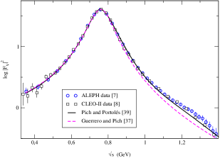
Figure 1: Comparison of the vector form factor of the pion as given by tau data and the theoretical description of Refs. [37, 39].

b) $1\,\mbox{GeV}\stackrel{{\scriptstyle<}}{{{}_{\sim}}}E\stackrel{{\scriptstyle<}}{{{}_{\sim}}}2\,\mbox{GeV}$
The extension of the description of the vector form factor of the pion at higher energies is cumbersome. Up to $2\,\mbox{GeV}$ two $\rho-$like resonances play the main role : $\rho(1450)$ and $\rho(1700)$. However the interference between resonances, the possible presence of a continuum component, etc. still deserve a study not yet done.

The inclusion of $\rho(1450)$ only improves slightly the behaviour when a Dyson-Schwinger-like resummation is performed in the framework of $R\chi T$ [30]. Lately, and based in a previous modelization proposed in Ref. [42], a procedure to extend the description of the vector form factor of the pion at higher energies has been put forward [21]. The proposal for the form factor embodies a Breit-Wigner parameterisation using both KS (7) and GS (8) models to describe $\rho(770)$, $\rho(1450)$ and $\rho(1700)$ resonances, appended with a modelization of large-$N_{C}$ QCD which sums up an infinite number of zero-width resonances to yield a Veneziano type of structure. In Fig. 2 it is shown how this parameterisation compares with data. The description is reasonable up to $2\,\mbox{GeV}$. Above this region there is almost no data though, in principle, it looks quite compatible with it [43].

Figure 2: Comparison of the vector form factor of the pion in the energy region above $1\,\mbox{GeV}$ from Ref. [21]. Solid (dashed) line corresponds to the KS (GS) parameterisation. See that reference for the explanation of data.

The all-important role that plays the vector form factor of the pion in the hadronic vacuum polarisation contribution to the anomalous magnetic moment of the pion [36], together with the seeming discrepancy between the predictions provided by $e^{+}e^{-}\rightarrow\pi^{+}\pi^{-}$ [44, 45] and $\tau^{-}\rightarrow\pi^{-}\pi^{0}\nu_{\tau}$ data, set up the issue of the size of isospin violation. A few years ago it was suggested [46] that the late excellent experimental determinations of the vector spectral functions in tau decay could be used to determine the hadronic vacuum polarisation contribution to $a_{\mu}$. The discrepancies that have arisen between the predictions from both sources were first blamed to the radiative corrections analyses in the first CMD-2 data, then to noticeable isospin violation unaccounted-for. A thorough analysis of the radiative corrections in $\tau^{-}\rightarrow\pi^{-}\pi^{0}\nu_{\tau}$ and other relevant isospin violating sources (kinematics, short-distance electroweak corrections, $\rho-\omega$ mixing) was carried out in Ref. [47]. As the variance persisted it was also claimed a strong isospin violation in the $\rho$ mass [48] though nor theory [49] nor other several determinations from experimental data [40, 41] seem to support it. Further analysis of the CMD-2 procedure detected several mistakes that have been corrected and are, at present, in agreement with recent KLOE data [45]. The matter is still open (see Ref. [50] for a recent account of this problem).

4 $\tau^{-}\rightarrow(\pi\pi\pi)^{-}\nu_{\tau}$ : Axial-vector form factors

The hadronic matrix element that drives the decay of the tau lepton into three pions is parameterised by four form factors $F_{i}$ defined as :

$$\left\langle\pi^{-0}(p_{1})\pi^{-0}(p_{2})\pi^{+-}(p_{3})\left|\,\left({\cal V}^{\mu}-{\cal A}^{\mu}\right)\,\right|0\right\rangle\,=$$

(14)

$$V^{\mu}_{1}F_{1}^{A}(Q^{2},s_{1},s_{2})\,+\,V^{\mu}_{2}F_{2}^{A}(Q^{2},s_{1},s_{2})$$

$$+\,Q^{\mu}\,F_{3}^{A}(Q^{2},s_{1},s_{2})\,+\,i\,V^{\mu}_{3}F_{4}^{V}(Q^{2},s_{1},s_{2})\,,$$

where

$$V^{\mu}_{1} = \left(g^{\mu\nu}-\frac{Q^{\mu}Q^{\nu}}{Q^{2}}\right)(p_{1}-p_{3})_{\nu}\,,$$

$$V^{\mu}_{2} = \left(g^{\mu\nu}-\frac{Q^{\mu}Q^{\nu}}{Q^{2}}\right)(p_{2}-p_{3})_{\nu}\,,$$

$$V^{\mu}_{3} = \varepsilon^{\mu\alpha\beta\gamma}p_{1\alpha}p_{2\beta}p_{3\gamma}\,,$$

$$Q^{\mu} = p_{1}^{\mu}+p_{2}^{\mu}+p_{3}^{\mu}\,,$$ (15)

$$s_{i} = \left(Q-p_{i}\right)^{2}\;.$$

This parameterisation is general for any three pseudoscalar final state. In the particular case at hand (three pions), we have, due to Bose-Einstein symmetry, that $F_{2}^{A}(Q^{2},s_{1},s_{2})=F_{1}^{A}(Q^{2},s_{2},s_{1})$. The scalar form factor $F_{3}^{A}$ vanishes with the mass of the Goldstone boson (chiral limit) and, accordingly, gives a tiny contribution in the three pion case. Finally the vector current only contributes if isospin symmetry is broken as demanded by G parity conservation; hence in the isospin limit $F_{4}^{V}=0$.

The final hadron system in the $\tau\rightarrow\pi\pi\pi\nu_{\tau}$ decays spans a wide energy region $3m_{\pi}\leq E\stackrel{{\scriptstyle<}}{{{}_{\sim}}}M_{\tau}$ that is heavily populated by resonances and has been thoroughly studied. In the very low energy regime the chiral constraints where explored in the seminal Ref. [51] and lately it has been calculated up to ${\cal O}(p^{4})$ in $\chi PT$ [35]. To account for the resonance energy region several modelizations given by phenomenological Lagrangians and vector meson dominance, matching the chiral behaviour, have been employed [35, 52]. However the most successful parameterisation has been the one given by the KS model [18, 19] that has been extendend to the study of all possible channels of three pseudoscalar mesons in the final state [20] and included in the TAUOLA Library [17].

The dynamics of $\tau\rightarrow\pi\pi\pi\nu_{\tau}$ is driven by the presence of the axial-vector $a_{1}(1260)$ modulated by the $I=1$ vector resonances $\rho(770)(\rho)$, $\rho(1450)(\rho^{\prime})$ and $\rho(1700)(\rho^{\prime\prime})$. Hence in the KS model the spin 1 axial-vector form factor is given by :

$$F_{1}^{A}(Q^{2},s_{i})={\cal N}|_{\chi{\cal O}(p^{2})}\,BW_{a_{1}}(Q^{2})\,\times$$

(16)

$$\times\;\frac{\displaystyle BW_{\rho}(s_{i})+\alpha\,BW_{\rho^{\prime}}(s_{i})\,+\,\beta\,BW_{\rho^{\prime\prime}}(s_{i})}{\displaystyle 1+\alpha+\beta}\;.$$

This description, complemented with an ad hoc construction of the off-shell width of the $a_{1}(1260)$ resonance, provides a good description of the spectrum of three pions [19] though a slight discrepancy shows up in the integrated structure functions [13]. The fit to the data gives the values of the $\alpha$ and $\beta$ parameters, that compute the weight of each $\rho$-like resonance and, in addition, one can study masses and on-shell widths of the participating resonances. The issue of isospin violation in this channel, within the KS model, has also been considered [53]. Lately it was shown that this Breit-Wigner parameterisation is not consistent with chiral symmetry at ${\cal O}(p^{4})$ and thus with QCD [33, 54].

A thorough study of the axial-vector form factors in $\tau\rightarrow\pi\pi\pi\nu_{\tau}$ has been performed in Ref. [33] using the methodology of effective field theories. The main components of this approach are :
1/ Resonance Chiral Theory
A Lagrangian theory provided by $R\chi T$ [26] has been employed. In this reference only linear terms in the resonances, whose couplings are under control, were introduced. In the decay of the tau into three pions, as commented above, a basic role is played by the interplay between the $a_{1}(1260)$ and $\rho$-like resonances. Accordingly it was necessary to construct, following chiral symmetry, a model-independent non-linear $a_{1}\rho\pi$ coupling that introduced 5 unknown couplings.
2/ Modelization of Large-$N_{C}$
Following the ideas of large-$N_{C}$ there were considered the tree level diagrams of the local Lagrangian theory. However this approach was corrected : first by cutting the infinite number of resonances that the leading $1/N_{C}$ expansion asks for, considering one octet of resonances only; then including off-shell widths for the $\rho(770)$ and $a_{1}(1260)$ according to the expressions given above, Eqs. (11,12), into the resonance propagators.
3/ Asymptotic behaviour of form factors
The high energy behaviour of the axial-vector spectral function at leading order in perturbative QCD [55] demands, heuristically, that the axial-vector form factors vanish at high $Q^{2}$, conclusion already collected into the Lepage-Brodsky leading behaviour of form factors [56]. This idea was used in order to provide two constraints on the 5 unknown couplings of the Lagrangian theory. Afterwards the evaluation of the Feynman diagrams constributing to $\tau\rightarrow\pi\pi\pi\nu_{\tau}$ showed that, once the constraints are enforced, only one combination of couplings is left unknown.
    Hence the authors get a parameterisation of the three pion decay of the tau lepton in terms of four free parameters : $M_{a_{1}}$, $\Gamma_{a_{1}}(M_{a_{1}})$, the combination of coupling constants and the $\alpha$ parameter in the off-shell width of the $a_{1}(1260)$ resonance. Next an analysis of the ALEPH data [10] on the spectrum and branching ratio of $\tau^{-}\rightarrow\pi^{+}\pi^{-}\pi^{-}\nu_{\tau}$ is performed. The fit is shown in Fig. 3 and they obtain $M_{a_{1}}=(1.204\pm 0.007)\,\mbox{GeV}$ and $\Gamma_{a_{1}}(M_{a_{1}}^{2})=(0.48\pm 0.02)\,\mbox{GeV}$ where the errors, given by the minimisation program, are only statistical.

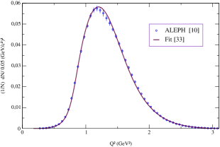
Figure 3: Fit to the ALEPH data [10] for the normalised $\tau^{-}\rightarrow\pi^{+}\pi^{-}\pi^{-}\nu_{\tau}$ decay [33].

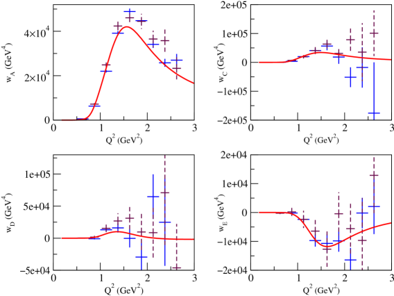
Figure 4: Theoretical predictions for the $w_{A}$, $w_{C}$, $w_{D}$ and $w_{E}$ integrated structure functions [33] in comparison with the experimental data from CLEO-II (solid) [13] and OPAL (dashed) [11].

OPAL [11] and CLEO [13] have collected data on the dominant structure functions in the $\tau^{-}\rightarrow\pi^{-}\pi^{0}\pi^{0}\nu_{\tau}$ decay, namely, $W_{A}$, $W_{C}$, $W_{D}$ and $W_{E}$ (5) that drive the contribution of the $J=1^{+}$ amplitude into the process and, accordingly, the integrated structure functions over all the available phase space, defined as :

$$w_{A,C}\,=\,\int\,ds_{1}\,ds_{2}\,W_{A,C}\;,$$ (17)

$$w_{D,E}\,=\,\int\,ds_{1}\,ds_{2}\,sign\left(s_{1}-s_{2}\right)\,W_{D,E}\;.$$ (18)

CLEO [13] displays the forecast given by the KS model and notice a slight discrepancy that shows up mainly in $w_{A}$. Then in order to have a better description they modify the model by supplying some quantum-mechanical structure (a heritage of nuclear physics that accounts for the finite size of hadrons) [57] that yields a good fit to data.

Following the results of the effective field theory approach explained above, and once the parameters are determined, it is possible to predict the integrated structure functions. By assuming isospin symmetry one can use the information obtained from the charged pions case to provide a description for the $\pi^{-}\pi^{0}\pi^{0}$ final hadronic state. The result and its comparison with the data is shown in Fig. 4. For $w_{C}$, $w_{D}$ and $w_{E}$, it can be seen that there is a good agreement in the low $Q^{2}$ region, while for increasing energy the experimental errors become too large to state any conclusion (moreover, there seems to be a little disagreement between both experiments at several points). On the other hand, in the case of $w_{A}$ the theoretical curve seems to lie somewhat below the data for $Q^{2}\stackrel{{\scriptstyle>}}{{{}_{\sim}}}1.5\,\mbox{GeV}^{2}$. However the study carried out in Ref. [33] seems to conclude that this is due to some inconsistency between the data by CLEO and OPAL, on one side, and ALEPH on the other. If the present data for $w_{A}$ is confirmed and the errors in the region of discrepancy lessen we will face a new structure not accounted for in the present theoretical description.

5 Prospects

Recently the CLEO Collaboration has published an analysis of the data collected on the $\tau^{-}\rightarrow K^{+}K^{-}\pi^{-}\nu_{\tau}$ decay [58]. It was known that this process is not well described by the KS model [59] and therefore in the new analysis they have reshaped the model with two new arbitrary parameters that modulate both one of the axial-vector and the vector form factors (4). Afterwards all the parameters are obtained through a reasonable fitting procedure. Along these pages we have emphasised the fact that arbitrary parameterisations are of little help in the procedure of obtaining information about non-perturbative QCD. It is usually claimed that the parameters hide physics that is not included specifically in the theory and they measure in fact our ignorance : the conclusion is that we may know how much ignorant we are but do not have a clue about the way out. In the CLEO example just pointed out the new parameter in the vector form factor spoils the Wess-Zumino anomaly normalisation, that appears at ${\cal O}(p^{4})$ in $\chi PT$. It is true that there are non-anomalous contributions proportional to the pseudoscalar masses at the next perturbative order that could account for a deviation but it would be surprising that the correction is around $80\%$ as the fit points out. The real issue is that, as we have indicated, the KS model is not consistent with QCD and the CLEO reshaping is of not much use.

Hadron decays of the tau lepton can provide all-important information on the hadronization of currents in order to yield relevant knowledge on non-perturbative features of low-energy Quantum Chromodynamics. In order to achieve this goal we need to input more controlled QCD-based modelizations. Our target is not only to fit the data at whatever cost, but do it with a reasonable parameterisation that allows us to understand more about the theoretical description of Nature.

The effective theory approach seems, along this line, more promising than the Breit-Wigner parameterisations. The procedure relies in a field theory construction that embodies, up to a supposedly minor modelization of the large-$N_{C}$ behaviour, the relevant features of QCD in the resonance energy region, giving an appropriate account of the main traits of the experimental data and showing that it is a compelling framework to work with. Notwithstanding it still has to probe its case with a complete study of, at least, all the three pseudoscalar channels.

Hadronic tau decays have undergone, during the last years, a fruitful era of excellence from the point of view of collecting experimental data. Experimentalists have done and are doing a great job. Now time has come for theoreticians to do their task.

References

- [1] S. Weinberg, Physica 96A (1979) 327.
- [2] J. Gasser and H. Leutwyler, Ann. Phys. (N.Y.) 158 (1984) 142; J. Gasser and H. Leutwyler, Nucl. Phys. 250 (1985) 465.
- [3] H. Georgi, Ann. Rev. Nucl. Part. Sci. 43 (1993) 209; A. Pich, Proceedings of Les Houches Summer School of Theoretical Physics, (Les Houches, France, 28 July-5 September 1997), edited by R. Gupta et al. (Elsevier Science, Amsterdam 1999), Vol. II, 949, hep-ph/9806303.
- [4] Ulf-G. Meissner, Phys. Rept. 161 (1988) 213; M. Bando, T. Kugo, K. Yamawaki, Phys. Rept. 164 (1988) 217.
- [5] G. Ecker, J. Gasser, H. Leutwyler, A. Pich and E. de Rafael, Phys. Lett. B223 (1989) 425.
- [6] J.H. Kühn and E. Mirkes, Z. Phys. C56 (1992) 661; J.H. Kühn and E. Mirkes, (E) idem C67 (1995) 364.
- [7] A. Rougé, Z. Phys. C70 (1996) 65; A. Rougé, Eur. Phys. J. C4 (1998) 265; R.J. Sobie, Phys. Rev. D60 (1999) 017301.
- [8] R. Barate et al, ALEPH Col., Z. Phys. C76 (1997) 15.
- [9] S. Anderson et al , CLEO Col., Phys. Rev. D61 (2000) 112002.
- [10] R. Barate et al, ALEPH Col., Eur. Phys. J. C4 (1998) 409.
- [11] K. Ackerstaff, OPAL Col., Z. Phys. C75 (1997) 593.
- [12] P. Abreu et al, DELPHI Col., Phys. Lett. 426 (1998) 411.
- [13] T.E. Browder et al, CLEO Col., Phys. Rev. D61 (1999) 052004.
- [14] K. Ackerstaff et al, OPAL Col., Eur. Phys. J. C7 (1999) 571.
- [15] K.W. Edwards et al, CLEO Col., Phys. Rev. D61 (2000) 072003.
- [16] F. Salvatore, these proceedings; R. Sobie, these proceedings.
- [17] R. Decker, S. Jadach, M. Jezabek, J.H. Kühn and Z. Was, Comput. Phys. Commun. 76 (1993) 361; ibid. 70 (1992) 69; ibid. 64 (1990) 275.
- [18] H. Kühn and F. Wagner, Nucl. Phys. B236 (1984) 16; A. Pich, Proceedings “Study of tau, charm and J/ physics development of high luminosity , Ed. L. V. Beers, SLAC (1989).
- [19] J.H. Kühn and A. Santamaría, Z. Phys. C48 (1990) 445.
- [20] R. Decker, E. Mirkes, R. Sauer and Z. Was, Z. Phys. C58 (1993) 445; R. Decker and E. Mirkes, Phys. Rev. D47 (1993) 4012; R. Decker, M. Finkemeier and E. Mirkes, Phys. Rev. D50 (1994) 6863; M. Finkemeier and E. Mirkes, Z. Phys. C69 (1996) 243; M. Finkemeier and E. Mirkes, Z. Phys. C72 (1996) 619.
- [21] C. Bruch, A. Khodjamirian and J.H. Kühn, hep-ph/0409080.
- [22] G.J. Gounaris and J.J. Sakurai, Phys. Rev. Lett. 21 (1968) 244.
- [23] H. Leutwyler, Ann. of Phys. (N.Y.) 235 (1994) 165.
- [24] G. t’Hooft, Nucl. Phys. B72 (1974) 461; E. Witten, Nucl. Phys. B160 (1979) 57.
- [25] S. Coleman and E. Witten, Phys. Rev. Lett. 45 (1980) 100.
- [26] G. Ecker, J. Gasser, A. Pich and E. de Rafael, Nucl. Phys. B321 (1989) 311.
- [27] D. Espriu, E. de Rafael and J. Taron, Nucl. Phys. B345 (1990) 22.
- [28] S. Weinberg, Phys. Rev. 166 (1968) 1568.
- [29] M. Knecht and A. Nyffeler, Eur. Phys. J. C21 (2001) 659; A. Pich, in Proceedings of the Phenomenology of Large QCD, edited by R. Lebed (World Scientific, Singapore, 2002), p. 239, hep-ph/0205030; G. Amorós, S. Noguera and J. Portolés, Eur. Phys. J. C27 (2003) 243; P.D. Ruiz-Femenía, A. Pich and J. Portolés, J. High Energy Physics 07 (2003) 003; V. Cirigliano, G. Ecker, M. Eidemüller, A. Pich and J. Portolés, Phys. Lett. B596 (2004) 96; J. Portolés and P.D. Ruiz-Femenía, Nucl. Phys. B (Proc. Suppl.) 131 (2004) 170.
- [30] J.J. Sanz-Cillero and A. Pich, Eur. Phys. J. C27 (2003) 587.
- [31] I. Rosell, J.J. Sanz-Cillero and A. Pich, J. High Energy Phys. 08 (2004) 042.
- [32] D. Gómez Dumm, A. Pich and J. Portolés, Phys. Rev. D62 (2000) 054014.
- [33] D. Gómez Dumm, A. Pich and J. Portolés, Phys. Rev. D69 (2004) 073002.
- [34] J. Gasser and H. Leutwyler, Nucl. Phys. B250 (1985) 517; J. Bijnens, G. Colangelo and P. Talavera, J. High Energy Phys. 05 (1998) 014; J. Bijnens and P. Talavera, J. High Energy Phys. 03 (2002) 046.
- [35] G. Colangelo, M. Finkemeier and R. Urech, Phys. Rev. D54 (1996) 4403; G. Colangelo, M. Finkemeier, E. Mirkes and R. Urech, Nucl. Phys. B (Proc. Suppl.) 55C (1997) 325; L. Girlanda and J. Stern, Nucl. Phys. B575 (2000) 285.
- [36] M. Davier, these proceedings.
- [37] F. Guerrero and A. Pich, Phys. Lett. B412 (1997) 382.
- [38] J.A. Oller, E. Oset and J.E. Palomar, Phys. Rev. D63 (2001) 114009.
- [39] A. Pich and J. Portolés, Phys. Rev. D63 (2001) 093005.
- [40] A. Pich and J. Portolés, Nucl. Phys. B (Proc. Suppl.) 121 (2003) 179.
- [41] J.F. de Trocóniz and F.J. Ynduráin, Phys. Rev. D65 (2002) 093001.
- [42] C.A. Dominguez, Phys. Lett. B512 (2001) 331.
- [43] J.H. Kühn, these proceedings.
- [44] R.R. Akhmetshin et al, CMD-2 Col., Phys. Lett. B527 (2002) 161.
- [45] A. Aloisio et al, KLOE Col., hep-ex/0407048; D. Leone, these proceedings.
- [46] R. Alemany, M. Davier and A. Höcker, Eur. Phys. J. C2 (1998) 123.
- [47] V. Cirigliano, G. Ecker and H. Neufeld, J. High Energy Phys. 08 (2002) 002.
- [48] S. Ghozzi and F. Jegerlehner, Phys. Lett. B583 (2004) 222.
- [49] J. Bijnens and P. Gosdzinsky, Phys. Lett. B388 (1996) 203.
- [50] M. Passera, hep-ph/0411168.
- [51] R. Fischer, J. Wess and F. Wagner, Z. Phys. 3 (1980) 313.
- [52] T. Berger, Z. Phys. 37 (1987) 95; M. Feindt, Z. Phys. 48 (1990) 681; E. Braaten, R.J. Oakes and S. Tse, Int. Journal of Mod. Phys. A5 (1990) 2737.
- [53] E. Mirkes and R. Urech, Eur. Phys. J. C1 (1998) 201.
- [54] J. Portolés, Nucl. Phys. B (Proc. Suppl.) 98 (2001) 210.
- [55] E.G. Floratos, S. Narison and E. de Rafael, Nucl. Phys. B155 (1979) 115.
- [56] S.J. Brodsky and G.R. Farrar, Phys. Rev. Lett. 31 (1973) 1153; G.P. Lepage and S.J. Brodsky, Phys. Rev. D22 (1980) 2157.
- [57] D.M. Asner et al, CLEO Col., Phys. Rev. D61 (2000) 012002.
- [58] T.E. Coan et al, CLEO Col., Phys. Rev. Lett. 92 (2004) 232001.
- [59] F. Liu, Nucl. Phys. B (Proc. Suppl.) 123 (2003) 66.