Spectator-model operators in point-form relativistic quantum mechanics

Abstract

We address the construction of transition operators for electromagnetic, weak, and hadronic reactions of relativistic few-quark systems along the spectator model. While the problem is of relevance for all forms of relativistic quantum mechanics, we specifically adhere to the point form, since it preserves the spectator character of the corresponding transition operators in any reference frame. The conditions imposed on the construction of point-form spectator-model operators are discussed and their implications are exemplified for mesonic decays of baryon resonances within a relativistic constituent quark model.

1 Introduction

Relativistic quantum mechanics (RQM) has been known for a long time as a feasible method to treat multi-particle systems in a Poincaré-invariant way Keister:1991sb . Already in 1949 Dirac described the front, instant, and point forms of relativistic dynamics Dirac:1949 . Based on a complete classification of subgroups of the Poincaré group, Leutwyler and Stern Leutwyler:1977vy also considered (the only) two further classes of RQM with a maximal transitive stability group. Most of the practical investigations in hadronic physics have been performed in the front and instant forms. Only in recent years the point form has attracted increasing attention. For instance, it has been applied to calculate the $\pi$ charge form factor Allen:1998hb , electromagnetic baryon form factors Coester:1997ih ; Berger:2005 , electroweak nucleon form factors Wagenbrunn:2000es ; Glozman:2001zc ; Boffi:2001zb ; Berger:2004yi , and also widths of $\pi$ and $\eta$ decay modes of $N$ and $\Delta$ resonances Melde:2002ga ; Melde:2004xj . In all cases a point-form spectator model (PFSM) Klink:1998pr has been adopted for the current and decay operators, respectively.

Tackling the full theory of a relativistic three-body system, including all genuine many-body operators required by Poincaré invariance (as well as hermiticity and current conservation) has not yet been possible in any one of the different forms of RQM mentioned above. Therefore one has resorted to simplified transition operators congruent with an impulse approximation in a nonrelativistic theory. However, this practice causes problems in RQM, since the constraints that have to be imposed on covariant relativistic operators lead to serious difficulties in the definition and application of one-body operators Polyzou:1986df ; Sengbusch:2004sf . Consequently, the constructions of so-called spectator-model operators are afflicted with specific shortcomings that have to be made up by additional ingredients. The latter usually turn spectator-model operators into effective many-body operators Polyzou:1986df ; Lev:1995wy .

The spectator-model approach in point-form has been found to be specific, since it preserves its spectator-model character in all reference frames Lev:1995wy . This property is connected with the fact that the generators of Lorentz transformations form the kinematic subgroup. As a result the PFSM can be made manifestly covariant. Certainly, this is a welcome behaviour for treating hadrons as relativistic few-quark systems.

The PFSM has been found to produce surprisingly good results, especially with regard to the elastic nucleon electroweak structure: the direct predictions by relativistic constituent quark models (CQM) have led to quite a consistent description of all the relevant observables in remarkable overall agreement with existing experimental data at low momentum transfers. In the PFSM relativistic (boost) effects definitely have big influences in all respects. A similar situation has been observed in the decay studies Melde:2002ga ; Melde:2004xj . The covariant predictions differ drastically from previous nonrelativistic or relativized results Stancu:1989iu ; Capstick:1993th ; Glozman:1998xs ; Theussl:2000sj . For the decays, however, the relativistic results systematically underestimate the experimental data and no satisfactory description is reached yet (with the simplistic decay models applied so far). The characteristics of the results found in the point-form approach have been seen in quite a similar manner with the relativistic CQM by the Bonn group Loring:2001kx ; Loring:2001ky in the framework of the Bethe-Salpeter equation Merten:2002nz ; Metsch:2003ix ; Metsch:2004qk .

The detailed properties of the point-form approach using PFSM operators have not yet been fully understood. There have been several studies to elucidate its behaviour, also in comparison to the spectator approximation of other forms of RQM Desplanques:2001zw ; Desplanques:2001ze ; Theussl:2003fs ; Coester:2003rw . Concrete calculations with realistic CQM wave functions comparing the point and instant forms in completely analogous spectator-model approaches have revealed big differences between them Berger:2005 ; Plessas:2004fn . Of course, the different forms of RQM are completely equivalent in a full calculation. Here, the question arises which contributions are effectively covered by the respective spectator-model approaches.

In this article, we deal with the fundamentals of defining PFSM operators. In particular, we investigate the implications of the basic symmetries of the Poincaré group for their construction. The problem is studied for general (elastic or inelastic) transitions. It is made clear that the PFSM in fact represents an effective many-body transition operator. Implications of different ways of spectator-model constructions in point form are demonstrated along concrete calculations of pionic decay widths of $N$ and $\Delta$ resonances for the case of the Goldstone-boson-exchange (GBE) CQM Glozman:1998ag ; Glozman:1998fs .

2 PFSM operators

The general translational-invariant amplitude between certain incoming and outgoing baryon states, $\left|V,M,J,\Sigma\right>$ and $\left<V^{\prime},M^{\prime},J^{\prime},\Sigma^{\prime}\right|$, is given by

$$\left<V^{\prime},M^{\prime},J^{\prime},\Sigma^{\prime}\right|{\hat{O}}\left|V,M,J,\Sigma\right>\\ =\left<V^{\prime},M^{\prime},J^{\prime},\Sigma^{\prime}\right|{\hat{O}}_{\rm rd}\left|V,M,J,\Sigma\right>\\ 2MV_{0}\delta^{3}\left(M{\vec{V}}-M^{\prime}{\vec{V}}^{\prime}-{\vec{Q}}\right)\,,$$ (1)

where $\hat{O}$ represents any electromagnetic, weak, or hadronic operator, and $\hat{O}_{\rm rd}$ is its reduced part. The baryon states are eigenstates of the four-velocity operator $\hat{V}$, the interacting mass operator $\hat{M}$, the (total) spin operator $\hat{J}$, and its z-component $\hat{\Sigma}$ (the corresponding letters without a hat denoting their eigenvalues). The factor in front of the $\delta$-function is the invariant measure ensuring the correct normalization and transformation properties of the states. The $\delta$-function itself expresses the overall momentum conservation of the transition amplitude under the four-momentum transfer $Q^{\mu}={P}^{\mu}-{P^{\prime}}^{\mu}$ (for on-shell particles). With the appropriate basis representations of the baryon eigenstates (see the Appendix) and inclusion of the necessary Lorentz transformations the expression for the transition amplitude becomes

$$\left<V^{\prime},M^{\prime},J^{\prime},\Sigma^{\prime}\right|{\hat{O}}\left|V,M,J,\Sigma\right>=$$

$$\frac{2}{MM^{\prime}}\sum_{\sigma_{i}\sigma^{\prime}_{i}}\sum_{\mu_{i}\mu^{\prime}_{i}}{\int{d^{3}{\vec{k}}_{2}d^{3}{\vec{k}}_{3}d^{3}{\vec{k}}^{\prime}_{2}d^{3}{\vec{k}}^{\prime}_{3}}}$$

$$\sqrt{\frac{\left(\omega_{1}+\omega_{2}+\omega_{3}\right)^{3}}{2\omega_{1}2\omega_{2}2\omega_{3}}}\sqrt{\frac{\left(\omega^{\prime}_{1}+\omega^{\prime}_{2}+\omega^{\prime}_{3}\right)^{3}}{2\omega^{\prime}_{1}2\omega^{\prime}_{2}2\omega^{\prime}_{3}}}$$

$$\Psi^{\star}_{M^{\prime}J^{\prime}\Sigma^{\prime}}\left({\vec{k}}^{\prime}_{1},{\vec{k}}^{\prime}_{2},{\vec{k}}^{\prime}_{3};\mu^{\prime}_{1},\mu^{\prime}_{2},\mu^{\prime}_{3}\right)$$

$$\prod_{\sigma^{\prime}_{i}}{D_{\sigma^{\prime}_{i}\mu^{\prime}_{i}}^{\star\frac{1}{2}}\left\{R_{W}\left[k^{\prime}_{i};B\left(V^{\prime}\right)\right]\right\}}$$

$$\left<p^{\prime}_{1},p^{\prime}_{2},p^{\prime}_{3};\sigma^{\prime}_{1},\sigma^{\prime}_{2},\sigma^{\prime}_{3}\right|{\hat{O}}_{\rm rd}\left|p_{1},p_{2},p_{3};\sigma_{1},\sigma_{2},\sigma_{3}\right>$$

$$\prod_{\sigma_{i}}{D_{\sigma_{i}\mu_{i}}^{\frac{1}{2}}\left\{R_{W}\left[k_{i};B\left(V\right)\right]\right\}}$$

$$\Psi_{MJ\Sigma}\left({\vec{k}}_{1},{\vec{k}}_{2},{\vec{k}}_{3};\mu_{1},\mu_{2},\mu_{3}\right)$$

$$2MV_{0}\delta^{3}\left(M{\vec{V}}-M^{\prime}{\vec{V}}^{\prime}-{\vec{Q}}\right)\,.$$ (2)

The integral measures stem from the completeness relation of the velocity states (see eq. (A10)), where the integrations over the velocities have already been performed exploiting the $\delta$-functions in the velocity-state representations of the baryon states (eq. (A11)). In this formula the individual quark momenta $\vec{k}_{i}$ (and similarly ${\vec{k}}^{\prime}_{i}$) are restricted by the rest-frame condition $\sum_{i}{{\vec{k}}_{i}}=\vec{0}$. The Wigner rotations stem from the Lorentz transformations to the boosted incoming and outgoing states, which have nonzero total momenta $\vec{P}=M{\vec{V}}$ and $\vec{P}^{\prime}=M^{\prime}{\vec{V}}^{\prime}$, respectively. The wave functions $\Psi^{\star}_{M^{\prime}J^{\prime}\Sigma^{\prime}}$ and $\Psi_{MJ\Sigma}$ denote the (rest-frame) velocity-state representations of the baryon states. The reduced operator ${\hat{O}}_{\rm rd}$ remains sandwiched between the free three-quark states.

At the outset ${\hat{O}}_{\rm rd}$ represents a general many-body operator. With present means the complete transition amplitude cannot be computed for any one of the reactions in question (electromagnetic, weak, or hadronic). Rather one has to resort to simplifications. Usually one first adopts a spectator model where the external particle couples only to one of the constituent quarks, while the other two are treated as spectators. In a nonrelativistic framework this would lead to a genuine one-body operator. However, this is not the case in a Poincaré-invariant theory. Observing all necessary constraints one arrives at effective many-body operators involving all quarks. This is basically true in all forms of RQM Polyzou:1986df ; Sengbusch:2004sf ; Lev:1995wy ; Simula:2001wx . Here we shall discuss the pertinent aspects especially for the point form.

The Graz group has applied spectator model operators in the point form to several processes. In case of electromagnetic reactions the PFSM for the current operator ${\hat{J}}^{\mu}_{\rm rd}$ reads Klink:1998pr ; Wagenbrunn:2000es ; Boffi:2001zb

$$\left<p^{\prime}_{1},p^{\prime}_{2},p^{\prime}_{3};\sigma^{\prime}_{1},\sigma^{\prime}_{2},\sigma^{\prime}_{3}\right|{\hat{J}}^{\mu}_{\rm rd}\left|p_{1},p_{2},p_{3};\sigma_{1},\sigma_{2},\sigma_{3}\right>=\\ 3{\cal N}\left<p^{\prime}_{1},\sigma^{\prime}_{1}\right|\hat{J}^{\mu}_{\rm spec}\left|p_{1},\sigma_{1}\right>\\ 2p_{20}\delta\left({\vec{p}}_{2}-{\vec{p}}^{\prime}_{2}\right)2p_{30}\delta\left({\vec{p}}_{3}-{\vec{p}}^{\prime}_{3}\right)\delta_{\sigma_{2}\sigma^{\prime}_{2}}\delta_{\sigma_{3}\sigma^{\prime}_{3}}\,,$$ (3)

where the matrix element of the spectator-quark current has a formal single-particle structure

$$\left<p^{\prime}_{1},\sigma^{\prime}_{1}\right|\hat{J}^{\mu}_{\rm spec}\left|p_{1},\sigma_{1}\right>=\\ e_{1}{\bar{u}}\left(p^{\prime}_{1},\sigma^{\prime}_{1}\right)\left[f_{1}({\tilde{Q}}^{2})\gamma^{\mu}+\frac{i}{2m_{1}}f_{2}({\tilde{Q}}^{2})\sigma^{\mu\nu}{\tilde{q}}_{\nu}\right]u\left(p_{1},\sigma_{1}\right)\,$$ (4)

with $f_{1}$ and $f_{2}$ being the Dirac form factors of the struck quark with mass $m_{1}$. Its spinor is expressed in terms of the usual two-component Pauli spinor $\chi$ in the following way

$$u(p,\sigma)=\sqrt{p_{0}+m}\left(\begin{array}[]{c}\chi\\ \\ \frac{\vec{\sigma}\cdot\vec{p}}{p_{0}+m}\,\,\chi\end{array}\right)\,.$$ (5)

The PFSM for the axial current is defined in an analogous manner Glozman:2001zc ; Boffi:2001zb

$$\left<p^{\prime}_{1},p^{\prime}_{2},p^{\prime}_{3};\sigma^{\prime}_{1},\sigma^{\prime}_{2},\sigma^{\prime}_{3}\right|{\hat{A}}^{\mu}_{a,\rm rd}\left|p_{1},p_{2},p_{3};\sigma_{1},\sigma_{2},\sigma_{3}\right>=\\ 3{\cal N}\left<p^{\prime}_{1},\sigma^{\prime}_{1}\right|\hat{A}^{\mu}_{a,{\rm spec}}\left|p_{1},\sigma_{1}\right>\\ 2p_{20}\delta\left({\vec{p}}_{2}-{\vec{p}}^{\prime}_{2}\right)2p_{30}\delta\left({\vec{p}}_{3}-{\vec{p}}^{\prime}_{3}\right)\delta_{\sigma_{2}\sigma^{\prime}_{2}}\delta_{\sigma_{3}\sigma^{\prime}_{3}}\,,$$ (6)

where the matrix element of the spectator-quark axial current is taken as

$$\left<p^{\prime}_{1},\sigma^{\prime}_{1}\right|\hat{A}^{\mu}_{a,{\rm spec}}\left|p_{1},\sigma_{1}\right>=\\ {\bar{u}}\left(p^{\prime}_{1},\sigma^{\prime}_{1}\right)\left[g_{A}^{q}\gamma^{\mu}+\frac{2f_{\pi}}{\widetilde{Q}^{2}+m_{\pi}^{2}}g_{qq\pi}\widetilde{q}^{\mu}\right]\gamma_{5}\frac{1}{2}{\tau}_{a}u\left(p_{1},\sigma_{1}\right)\,$$ (7)

with $m_{\pi}$ the pion mass, $f_{\pi}$ the pion decay constant, $g_{A}^{q}=1$ the quark axial charge, $g_{qq\pi}$ the pion-quark coupling constant, and ${\tau}_{a}$ the isospin matrix with Cartesian index $a$.

For the mesonic decays of baryon resonances a decay model has been assumed with an elementary pseudovector coupling of the meson being directly emitted from a single quark. The corresponding PFSM operator has the following structure Melde:2002ga ; Melde:2004ce

$$\left<p^{\prime}_{1},p^{\prime}_{2},p^{\prime}_{3};\sigma^{\prime}_{1},\sigma^{\prime}_{2},\sigma^{\prime}_{3}\right|{\hat{D}}_{m,{\rm rd}}\left|p_{1},p_{2},p_{3};\sigma_{1},\sigma_{2},\sigma_{3}\right>=\\ 3{\cal N}\frac{ig_{qqm}}{2m_{1}\left(2\pi\right)^{\frac{3}{2}}}{\bar{u}}\left(p^{\prime}_{1},\sigma^{\prime}_{1}\right)\gamma_{5}\gamma^{\mu}\lambda_{m}u\left(p_{1},\sigma_{1}\right)Q_{\mu}\\ 2p_{20}\delta\left({\vec{p}}_{2}-{\vec{p}}^{\prime}_{2}\right)2p_{30}\delta\left({\vec{p}}_{3}-{\vec{p}}^{\prime}_{3}\right)\delta_{\sigma_{2}\sigma^{\prime}_{2}}\delta_{\sigma_{3}\sigma^{\prime}_{3}}\,$$ (8)

with the flavor matrix $\lambda_{m}$ characterizing the particular decay mode and $g_{qqm}$ representing the corresponding quark-meson coupling constant.

In eqs. (4) and (7) ${\tilde{q}}^{\mu}$ denotes the momentum transfer to the struck quark in the Breit frame

$${\tilde{q}}^{\mu}={p}^{\mu}_{1}-{p^{\prime}}^{\mu}_{1}\,\,\,\,\,,\,\,\,\,\,{\tilde{q}}^{\mu}{\tilde{q}}_{\mu}=-{\tilde{Q}^{2}}\,.$$ (9)

It is different from the momentum $Q^{\mu}$ transferred to the baryon as a whole. Only part of the total momentum is transferred to the struck quark. Even though the external particle (the photon or the intermediate boson) couples only to a single quark, also the spectator quarks participate in the process since the total-momentum operator $\hat{P}$ is dynamical. This makes the PFSM current an effective many-body current. The same consideration holds for the decay process when the meson is emitted from a single quark. In all cases ${\tilde{q}}^{\mu}$ is completely fixed by the two spectator conditions and the overall momentum conservation, and there is no arbitrariness.

The PFSM currents in eqs. (4) and (7) maintain their spectator-model character in all reference frames Lev:1995wy . This is simply a consequence of the fact that the generators of Lorentz transformations are kinematical in the point form. The constructions of the electroweak currents and likewise of the decay operator in eq. (8) themselves are Lorentz-invariant and the spectator conditions are given by invariant $\delta$-functions. The Lorentz-covariance of the spectator-model operators does not exist in the other forms of RQM. It is a specific property of the point form Coester1995ic .

In eqs. (3), (6), and (8) there occurs a normalization factor $\cal N$ for all PFSM operators. In the electromagnetic case it is needed to reproduce the proton charge (the electric form factor at zero momentum transfer). For consistency reasons the same construction should be adopted also for the weak and hadronic operators. The Graz group made the choice

$${\cal N}={\cal N}_{\rm S} = \left(\frac{M}{\sum_{i}{\omega_{i}}}\frac{M^{\prime}}{\sum_{i}{\omega^{\prime}_{i}}}\right)^{\frac{3}{2}}\,.$$ (10)

In this way, $\cal N$ is assumed in a Lorentz-invariant form. This maintains the manifest covariance of the point-form transition amplitudes in the spectator model. From eq. (10) it is also seen that the normalization factor depends on the interactions, since $M$ and $M^{\prime}$ are the eigenvalues of the interacting mass operator (of the incoming and outgoing baryons). The ratios of the interacting mass eigenvalue to the sum of the individual quark energies in the denominator are chosen in a symmetric manner for both the incoming and outgoing channels. It should be noted that in the integration of the matrix element in eq. (2) the sums of the individual quark energies in $\cal N$ enter as functions of the integration variables and thus indirectly introduce a certain dependence on the momentum transfer $Q$ in the final results.

With the use of eq. (10) for $\cal N$, accounting for charge normalization in a Poincaré-invariant PFSM, one achieved a very reasonable description of the elastic electroweak nucleon structure with both the relativistic Goldstone-boson-exchange and one-gluon-exchange CQMs Plessas:2004fn . In particular, the momentum dependence of the electromagnetic and axial form factors could be well reproduced by the PFSM for momentum transfers up to $Q^{2}\sim 5$ GeV².

The choice of the normalization factor $\cal N$, however, is not unique at this point. Under the assumptions of Poincaré invariance and charge normalization several other possibilities exist. This has to be considered especially in the context of inelastic processes. Here one could also think of choices other than the symmetric one. In the following we investigate the origin of the normalization factor and study the implications of alternative forms in case of the mesonic decays of $N$ and $\Delta$ resonances.

3 Spectator Conditions and Translational Invariance

In order to get a better insight into the nature of the normalization factor $\cal N$ let us now shed some more light on the interplay of the spectator $\delta$-functions and the overall-momentum conserving $\delta$-function in the expression for the matrix element of the transition amplitude in eq. (2). This investigation will also further elucidate the role of ${\tilde{q}}^{\mu}$ and the proportioning of the whole momentum transfer among the individual quarks.

In point form we have

$${\hat{P}}_{\rm free}={\hat{M}}_{\rm free}{\hat{V}}_{\rm free}$$ (11)

for the free system and

$$\hat{P}=\hat{M}{\hat{V}}_{\rm free}$$ (12)

for the interacting system according to the Bakamjian-Thomas construction Bakamjian:1953 . The four-velocity remains kinematical upon introducing the interactions. As a consequence the momentum and mass eigenvalues of the free and interacting systems are constrained by

$$V_{\rm free}=\frac{P_{\rm free}}{M_{\rm free}}=\frac{\sum_{i}{p_{i}}}{\sum_{i}{\omega_{i}}}=\frac{P}{M}=V\,.$$ (13)

However,

$$\sum_{i}{p_{i}}\neq P=MV\,.$$ (14)

Remember that in point form the mass and the four-momentum operators are the only operators affected by interactions. All other generators of the Poincaré algebra remain kinematical.

Next we exploit the relation (13) for the overall-momentum conserving $\delta$-function. Since it is an invariant form, we can consider it in any reference frame. Let us assume we are working in the rest frame of the incoming baryon, where $\sum_{i}{{\vec{p}}_{i,\rm in}}={\vec{0}}$. For this particular case we denote all frame-dependent quantities with the index ‘$\rm in$’. Then we can write the invariant $\delta$-function as

$$2MV_{0}\delta^{3}\left(M{\vec{V}}-M^{\prime}{\vec{V}}^{\prime}-{\vec{Q}}\right)$$

$$=2MV_{0,\rm in}\delta^{3}\left(M{\vec{V}}_{\rm in}-M^{\prime}{\vec{V}}^{\prime}_{\rm in}-{\vec{Q}}_{\rm in}\right)$$

$$=2MV_{0,\rm in}\delta^{3}\left(-M^{\prime}\frac{\sum_{i}{{\vec{p}}^{\prime}_{i,\rm in}}}{\sum_{i}{\omega^{\prime}_{i}}}-{\vec{Q}}_{\rm in}\right)$$ (15)

$$=2MV_{0,\rm in}\left(\frac{\sum_{i}{\omega^{\prime}_{i}}}{M^{\prime}}\right)^{3}\delta^{3}\left(-\sum_{i}{{\vec{p}}^{\prime}_{i,\rm in}}-\frac{\sum_{i}{\omega^{\prime}_{i}}}{M^{\prime}}{\vec{Q}}_{\rm in}\right)\,.$$

Utilizing the spectator conditions, $\vec{p}^{\prime}_{2,\rm in}=\vec{p}_{2,\rm in}$ and $\vec{p}^{\prime}_{3,\rm in}=\vec{p}_{3,\rm in}$, this finally leads to the result

$$2MV_{0,\rm in}\delta^{3}\left(M{\vec{V}}_{\rm in}-M^{\prime}{\vec{V}}^{\prime}_{\rm in}-{\vec{Q}}_{\rm in}\right)\\ =2MV_{0,\rm in}\left(\frac{\sum_{i}{\omega^{\prime}_{i}}}{M^{\prime}}\right)^{3}\delta^{3}\left({\vec{p}}_{1,\rm in}-{\vec{p}}^{\prime}_{1,\rm in}-\frac{\sum_{i}{\omega^{\prime}_{i}}}{M^{\prime}}{\vec{Q}}_{\rm in}\right)\,,$$ (16)

where ${V}_{0,\rm in}=1$ in this particular frame.

It is immediately evident that the momentum transfer to the struck quark is not the same as the momentum transfer to the baryon as a whole:

$$\frac{\sum_{i}{\omega^{\prime}_{i}}}{M^{\prime}}{\vec{Q}}_{\rm in}={\tilde{\vec{q}}}_{\rm in}\neq\vec{Q}_{\rm in}\,.$$ (17)

The difference can be expressed as

$$\vec{Q}_{\rm in}-{\tilde{\vec{q}}}_{\rm in}=\frac{M^{\prime}-\sum_{i}{\omega_{i}}^{\prime}}{M^{\prime}}{\vec{Q}}_{\rm in}=\frac{M^{\prime}-M^{\prime}_{\rm free}}{M^{\prime}}{\vec{Q}}_{\rm in}\,.$$ (18)

Obviously, it depends on the energies (and thus momenta) of all three quarks and therefore makes the PFSM operator an effective many-body operator.

It is also interesting to observe that the difference between the momentum transfers $\vec{Q}_{\rm in}$ and ${\tilde{\vec{q}}}_{\rm in}$ is determined by the difference between the interacting and the free mass operators of the outgoing baryon, i.e. the interaction responsible for its binding.

Now we notice the factor in front of the $\delta$-function in the last line of eq. (16). Its nature resembles the inverse of the normalization factor $\cal N$ used in the definition of the PFSM operators in eq. (10). Only it is not symmetric in the mass eigenvalues of the incoming and outgoing baryons. However, it can be utilized for defining another normalization factor

$${\cal N}_{\rm in}=\left(\frac{M^{\prime}}{\sum_{i}{\omega^{\prime}_{i}}}\right)^{3}\,,$$ (19)

which would also work in the construction of the PFSM operators. In particular, it would guarantee for the correct proton charge normalization and fulfill all the other constraints of Poincaré invariance. Of course, the normalization factor ${\cal N}_{\rm in}$ produces a momentum dependence of the results different from the one of ${\cal N}_{\rm S}$.

We can repeat the above procedure with the overall-momentum conserving $\delta$-function in the rest-frame of the outgoing baryon, where $\sum_{i}{{\vec{p}}^{\prime}_{i,\rm out}}={\vec{0}}$ and the index ‘$\rm out$’ now denotes the frame-dependent variables in this specific frame. We obtain instead of eq. (16) the result

$$2M{V}_{0}\delta^{3}\left(M{\vec{V}}-M^{\prime}{\vec{V}}^{\prime}-{\vec{Q}}\right)$$

$$=2MV_{0,\rm out}\delta^{3}\left(M{\vec{V}}_{\rm out}-M^{\prime}{\vec{V}}^{\prime}_{\rm out}-{\vec{Q}}_{\rm out}\right)$$ (20)

$$=2M{V}_{0,\rm out}\left(\frac{\sum_{i}{\omega_{i}}}{M}\right)^{3}\delta^{3}\left({\vec{p}}^{\prime}_{1,\rm out}-{\vec{p}}_{1,\rm out}-\frac{\sum_{i}{\omega_{i}}}{M}{\vec{Q}}_{\rm out}\right).$$

Again, the momentum transfer to the struck quark is not the same as the momentum transfer to the baryon as a whole

$$\frac{\sum_{i}{\omega_{i}}}{M}{{\vec{Q}}_{\rm out}}={\tilde{\vec{q}}}_{\rm out}\neq{\vec{Q}}_{\rm out}\,,$$ (21)

where their difference now depends on the masses in the incoming channel

$${\vec{Q}}_{\rm out}-{\tilde{\vec{q}}}_{\rm out}=\frac{M-\sum_{i}{\omega_{i}}}{M}{{\vec{Q}}_{\rm out}}=\frac{M-M_{\rm free}}{M}{{\vec{Q}}_{\rm out}}\,.$$ (22)

We note that in general ${\tilde{\vec{q}}}_{\rm out}$ is different from ${\tilde{\vec{q}}}_{\rm in}$. The portion of momentum transfer to the struck quark changes with the reference frame. The final result for any transition amplitude, however, does not. It is covariant in point form.

The factor in front of the $\delta$-function in the last line of eq. (3) suggests again another normalization factor

$${\cal N}_{\rm out}=\left(\frac{M}{\sum_{i}{\omega_{i}}}\right)^{3}\,.$$ (23)

It would similarly be suited in the construction of PFSM operators just like ${\cal N}_{\rm S}$ and ${\cal N}_{\rm in}$.

At this point all three normalization factors ${\cal N}_{\rm S}$, ${\cal N}_{\rm in}$, and ${\cal N}_{\rm out}$ meet the requirements posed so far, namely, Poincaré invariance and charge normalization. Therefore we have to notice an ambiguity. In the next section we shall investigate the implications of the different possible choices in the mesonic decays of $N$ and $\Delta$ resonances, where we have different particles in the incoming and outgoing channels.

4 $\cal N$ Dependence of Decay Widths

Let us assume for the normalization factor $\cal N$ the general form

$${\cal N}\left(y\right)=\left(\frac{M}{\sum_{i}{\omega_{i}}}\right)^{3y}\left(\frac{M^{\prime}}{\sum_{i}{\omega^{\prime}_{i}}}\right)^{3\left(1-y\right)}\,.$$ (24)

with $0\leq y\leq 1$. It contains all of the three forms, ${\cal N}_{\rm S}$, ${\cal N}_{\rm in}$, and ${\cal N}_{\rm out}$, discussed in the previous section and it also meets all the requirements posed (Poincaré invariance and charge normalization). We emphasize that the transition amplitudes are covariant for every particular fixed $y$. However, the results will vary for different values of the asymmetry parameter $y$ .

We studied the decay widths of $N$ and $\Delta$ resonances with the PFSM decay operator of eq. (8). The actual computations were performed in the rest frame of the decaying resonance. We emphasize, however, that the PFSM results are frame-independent. In table 1 we first demonstrate the dissimilarity of the predictions in case of the GBE CQM for either one of the choices ${\cal N}_{\rm S}$, ${\cal N}_{\rm in}$, and ${\cal N}_{\rm out}$. It is seen that the normalization factor ${\cal N}_{\rm in}$ yields the smallest values of the decay widths in all cases. Contrary to that, ${\cal N}_{\rm out}$ always produces the biggest predictions. The symmetric ${\cal N}_{\rm S}$ is intermediate between the two. In the last column of table 1 we have also quoted the results that would be obtained if $\cal N$ was left out completely; we denoted this case by ${\cal N}_{\rm bare}$. It does not meet the requirement of (proton) charge normalization in the electroweak sector. Obviously, the corresponding results are completely unreasonable also here for the decay widths.

When considering the different predictions in table 1 we notice that the normalization factor ${\cal N}_{\rm out}$ leads to an overestimation of the experimental data in several cases. This drawback is avoided completely by ${\cal N}_{\rm S}$. The corresponding results always remain smaller than the experimental data or do not exceed them. We consider this to be a reasonable feature, since a more elaborate decay model than the one used here would tentatively bring in additional contributions that are expected to make the predictions bigger and thus get them into closer agreement with the data. The results with ${\cal N}_{\rm in}$ are always much too small as compared to experiment.

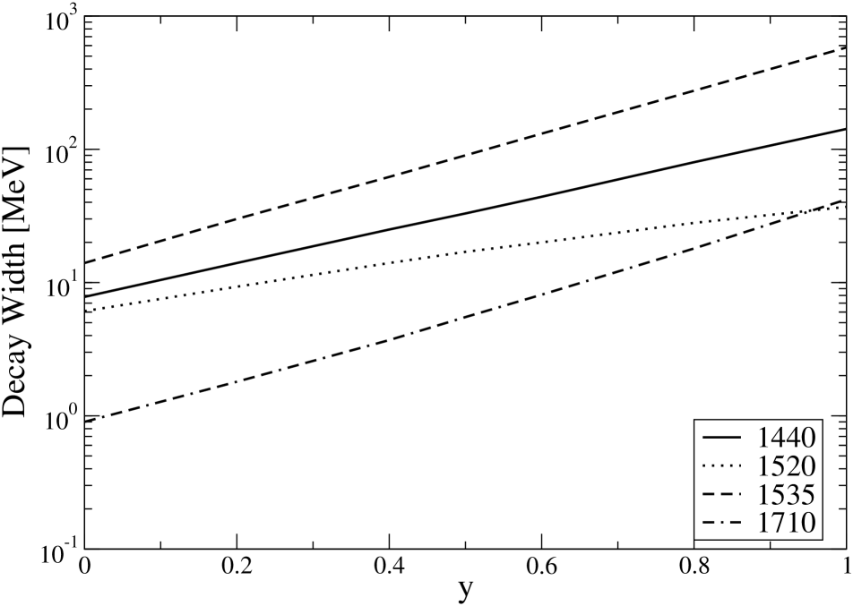
Figure 1: Dependence of the $\pi$ decay widths on the asymmetry parameter $y$ in the normalization factor of eq. (24) for selected $N$ resonances.

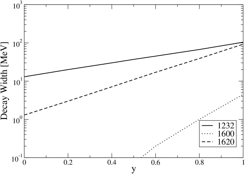
Figure 2: Dependence of the $\pi$ decay widths on the asymmetry parameter $y$ in the normalization factor of eq. (24) for selected $\Delta$ resonances.

The detailed dependence of the results on the asymmetry parameter $y$ in eq. (24) is demonstrated in table 2. A smooth transition of the theoretical values from $y=0$ (corresponding to ${\cal N}_{\rm in}$) via $y=0.5$ (corresponding to ${\cal N}_{\rm S}$) to $y=1$ (corresponding to ${\cal N}_{\rm out}$) is observed for all resonance decays. We have exemplified this behaviour for some of the $N$ and $\Delta$ resonances in figs. 1 and 2, respectively. There is practically an exponential rise of the theoretical values when $y$ varies from zero to one.

From these studies one learns that the normalization factors modify the dependence on the recoil, i.e. on the $Q$-dependence in eq. (8). It is noteworthy that the symmetric choice ${\cal N}_{\rm S}$, which was originally adopted as the optimal one in the electroweak case, also leads to the most reasonable results in the hadronic decays considered here (in the sense that the experimental data are not overestimated).

That the normalization factor $\cal N$ in eqs. (3), (6), and (8) effectively introduces a momentum cut-off can even better be seen if we investigate the form

$${\cal N}\left(x\right)=\left(\frac{M}{\sum_{i}{\omega_{i}}}\frac{M^{\prime}}{\sum_{i}{\omega^{\prime}_{i}}}\,\right)^{\frac{x}{2}}\,$$ (25)

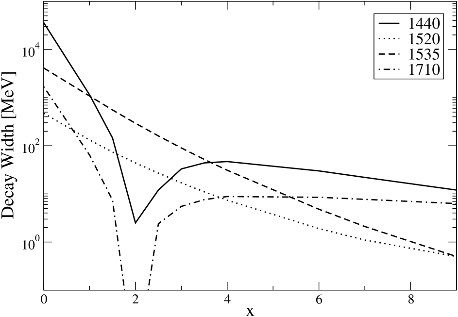
Figure 3: Dependence of the $\pi$ decay widths on the exponent $x$ of the normalization factor in eq. (25) for selected $N$ resonances.

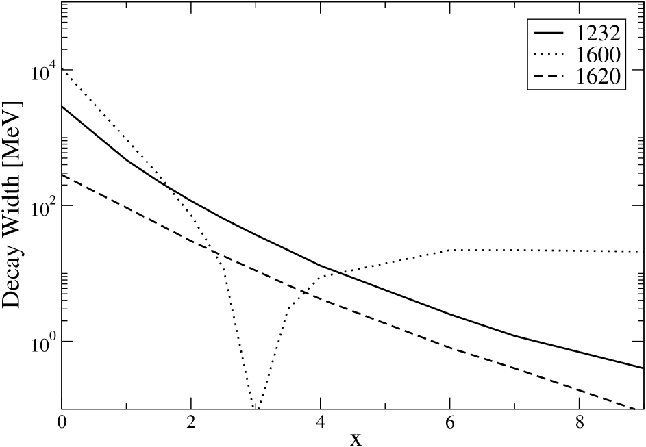
Figure 4: Dependence of the $\pi$ decay widths on the exponent $x$ of the normalization factor in eq. (25) for selected $\Delta$ resonances.

with an arbitrary exponent $x$. It still represents a Poincaré-invariant construction but it does not guarantee for the proper charge normalization unless $x=3$. It is instructive to look at the predictions for decay widths as a function of the exponent $x$ in table 3. Starting out from the (unreasonable) bare case the theoretical results evolve smoothly with increasing exponent $x$. For $x=3$ we recover the predictions for ${\cal N}_{\rm S}$ in table 1. For certain resonances the decay widths have a minimum. This is exemplified in figs. 3 and 4. We notice that the minima occur just for the resonances $N(1440)$, $N(1710)$, and $\Delta(1600)$, which are known as the so-called structure-dependent resonances Koniuk:1980vy . They are the radial excitations of the $N$ and $\Delta$ ground states, respectively, with a corresponding nodal behaviour in their wave functions. These characteristics are quite distinct from the other resonances, which show a monotonous dependence on the exponent $x$.

If we assume again the criterion that the theoretical predictions for decay widths with the decay operator (8) should not exceed the experimental data, we find as the optimal case the one with $x=3$. In this way we are led back to the assumption of the symmetric normalization factor in eq. (10), which also meets all the theoretical requirements imposed.

5 Summary

We have investigated the spectator-model construction of transition operators in point form. Based on the explicit forms of the current operators for electromagnetic as well as weak reactions and the decay operator for baryon resonances we have investigated the specific ingredients in the PFSM. We have made transparent the effective many-body nature of the spectator-model operator in point form. In particular, we have explained the distribution of the total momentum transfer $Q$ among the constituent quarks in a baryon through the Lorentz boosts under the constraint of translational invariance. As a result the momentum $\tilde{q}$ transferred to the struck quark is only a part of the total $Q$. Furthermore we have devoted our attention to the definition of the normalization factor $\cal N$ occurring in the PFSM operators. We noticed that several choices are possible even under the constraints of charge normalization (in the electroweak case) and Poincaré invariance. However, the final results depend on the particular choice made. Therefore in any PFSM calculation it should be specified which normalization factor has been adopted.

The influence of different normalization factors has been investigated with regard to pionic decays of $N$ and $\Delta$ resonances. In the concrete calculations we have employed the wave functions as produced by the GBE CQM. Qualitatively the results would be quite similar with other realistic baryon wave functions, e.g., the ones from a one-gluon-exchange CQM (see ref. Melde:2004xj , where the influences of different dynamics on decay widths have been discussed). We have demonstrated the modification of the momentum dependence that is introduced by different choices of $\cal N$. Upon comparing the theoretical predictions with experiment we have found a preference for the symmetric choice ${\cal N}_{\rm S}$ in the PFSM decay operator adopted here. This observation is congruent with the one made in the electroweak sector. With regard to the pionic decays, however, even the calculation with ${\cal N}_{\rm S}$ using the wave functions of the GBE CQM and the present PFSM decay operator does not produce a satisfactory description of the experimental data.

While our investigations have been made specifically for the point form, most of the questions addressed here are also relevant for the other forms of RQM in case spectator operators are considered. Similar problems occur in the instant and front forms if the necessary invariance constraints are imposed (cf., for instance, refs. Polyzou:1986df ; Lev:1995wy ; Simula:2001wx ; Keister:1994mg ; Lev:2000vm ; Desplanques:2004zp ). In some respects even additional complications arise connected with the fact that Lorentz transformations are no longer kinematical. For example, in instant form the spectator-model character of any operator constructed in one frame will not be maintained under Lorentz transformations. In any other reference frame specific genuine many-body operators will be generated.

Here, and in previous works, we have seen certain advantages of the point-form approach in the treatment of relativistic few-body problems. The PFSM construction definitely includes effective contributions from many-body operators. Their sources are twofold. They stem from the sharing of the total momentum transfer to the individual quarks and from the necessary normalization factor $\cal N$, which involves the interacting mass operators. The different possible choices of $\cal N$ constitute a quantitatively significant ambiguity. It is important to take these peculiarities of the PFSM into account before going to include explicit many-body operators.

Appendix:
States and Wave Functions in Point Form RQM

In RQM baryon states are expressed as eigenstates $\left|P,J,\Sigma\right>$ of the four-momentum $\hat{P}$, total spin $\hat{J}$, and its $z$-component $\hat{\Sigma}$ (the letters without hat denoting the corresponding eigenvalues). Their covariant normalization is

$$\left<P^{\prime},J^{\prime},\Sigma^{\prime}|P,J,\Sigma\right>=2P_{0}\delta^{3}\left({\vec{P}}-{\vec{P}}^{\prime}\right)\delta_{JJ^{\prime}}\delta_{\Sigma\Sigma^{\prime}}\,.$$ (A1)

The baryon states can equivalently be expressed by $\left|V,M,J,\Sigma\right>$, i.e. as eigenstates of the four-velocity operator $\hat{V}$, the (interacting) mass operator $\hat{M}$ as well as $\hat{J}$ and $\hat{\Sigma}$. For the eigenvalues of the four-vector $V$ one always has the constraint $V^{\mu}V_{\mu}=1$. The covariant normalization of the baryon states $\left|V,M,J,\Sigma\right>$ reads

$$\left<V^{\prime},M^{\prime},J^{\prime},\Sigma^{\prime}|V,M,J,\Sigma\right>\\ =2MV_{0}\delta^{3}\left(M{\vec{V}}-M^{\prime}{\vec{V}}^{\prime}\right)\delta_{JJ^{\prime}}\delta_{\Sigma\Sigma^{\prime}}\,.$$ (A2)

For the baryon wave functions the eigenstates can be expressed in different basis representations. One basis is provided by the free three-particle states, which are tensor products of one-particle states. Their covariant normalization is

$$\left<p^{\prime}_{1},p^{\prime}_{2},p^{\prime}_{3};\sigma^{\prime}_{1}\sigma^{\prime}_{2},\sigma^{\prime}_{3}|p_{1},p_{2},p_{3};\sigma_{1}\sigma_{2},\sigma_{3}\right>\\ =2p_{10}\delta^{3}\left({\vec{p}}_{1}-{\vec{p}}^{\prime}_{1}\right)2p_{20}\delta^{3}\left({\vec{p}}_{2}-{\vec{p}}^{\prime}_{2}\right)2p_{30}\delta^{3}\left({\vec{p}}_{3}-{\vec{p}}^{\prime}_{3}\right)\\ \times\delta_{\sigma_{1}\sigma^{\prime}_{1}}\delta_{\sigma_{2}\sigma^{\prime}_{2}}\delta_{\sigma_{3}\sigma^{\prime}_{3}}\,,$$ (A3)

and their completeness relation reads

$$1=\sum_{\sigma_{1},\sigma_{2},\sigma_{3}}\int{\frac{d^{3}{\vec{p}}_{1}}{2p_{10}}\frac{d^{3}{\vec{p}}_{2}}{2p_{20}}\frac{d^{3}{\vec{p}}_{3}}{2p_{30}}}\\ \left|p_{1},p_{2},p_{3};\sigma_{1},\sigma_{2},\sigma_{3}\right>\left<p_{1},p_{2},p_{3};\sigma_{1},\sigma_{2},\sigma_{3}\right|\,.$$ (A4)

For on-shell particles out of the 12 momentum components only 9 remain as integration variables. In the rest frame we write these states as $\left|k_{1},k_{2},k_{3};\mu_{1},\mu_{2},\mu_{3}\right>$, where $\sum_{i}{{\vec{k}}_{i}}=\vec{0}$.

Another basis is provided by the so-called velocity states (of the free system). They are advantageous in practical caluclations and have already been used before, among others in refs. Klink:1998hc ; Krassnigg:2003gh , with slightly different normalizations. We define them by

$$\left|v;\vec{k}_{1},\vec{k}_{2},\vec{k}_{3};\mu_{1},\mu_{2},\mu_{3}\right\rangle=U_{B(v)}\left|k_{1},k_{2},k_{3};\mu_{1},\mu_{2},\mu_{3}\right\rangle$$

$$=\sum_{\sigma_{1},\sigma_{2},\sigma_{3}}\prod\limits_{i=1}^{3}D^{\frac{1}{2}}_{\sigma_{i}\mu_{i}}[R_{W}(k_{i},B(v))]\left|p_{1},p_{2},p_{3};\sigma_{1},\sigma_{2},\sigma_{3}\right\rangle\,.$$

(A5)

Here $B\left(v\right)$, with unitary representation $U_{B\left(v\right)}$, is a boost with four-velocity $v$ on the three-body states $\left|k_{1},k_{2},k_{3};\mu_{1},\mu_{2},\mu_{3}\right\rangle$ in the rest frame. The relation between $p_{i}$ and $k_{i}$ is thus given by

$$p_{i}=B\left(v\right)k_{i}\,,$$ (A6)

and the four-velocity is expressed by

$${v}=\frac{\sum_{i}{{p}_{i}}}{M_{\rm free}}=\frac{\sum_{i}{{p}_{i}}}{\sum_{i}{\omega_{i}}}\,,$$ (A7)

where $M_{\rm free}$ is the invariant free mass and $\omega_{i}=\sqrt{{\vec{k}}_{i}^{2}+m_{i}^{2}}$ are the energies of the individual quarks with mass $m_{i}$. In case of the velocity states one has $\vec{v}$ and two of the three quark momenta, $\vec{k}_{2}$ and $\vec{k}_{3}$, say, as the 9 independent variables. The transformation from the free three-body states to the free velocity states is given by the Jacobi determinant

$${\cal J}\left\{\frac{\partial\left({\vec{p}}_{1},{\vec{p}}_{2},{\vec{p}}_{3}\right)}{\partial\left({\vec{v}},{\vec{k}}_{2},{\vec{k}}_{3}\right)}\right\}=\frac{2p_{10}2p_{20}2p_{30}\left(\omega_{1}+\omega_{2}+\omega_{3}\right)^{3}}{2\omega_{1}2\omega_{2}2\omega_{3}v_{0}}\,.$$ (A8)

Due to eqs. (A3) and (A4) it implies the following normalization

$$\left\langle v;\vec{k}_{1},\vec{k}_{2},\vec{k}_{3};\mu_{1},\mu_{2},\mu_{3}|v^{\prime};\vec{k}^{\prime}_{1},\vec{k}^{\prime}_{2},\vec{k}^{\prime}_{3};\mu^{\prime}_{1},\mu^{\prime}_{2},\mu^{\prime}_{3}\right\rangle\\ =\frac{2\omega_{1}2\omega_{2}2\omega_{3}}{\left(\omega_{1}+\omega_{2}+\omega_{3}\right)^{3}}\delta_{\mu_{1}\mu^{\prime}_{1}}\delta_{\mu_{2}\mu^{\prime}_{2}}\delta_{\mu_{3}\mu^{\prime}_{3}}\\ \times v_{0}\delta^{3}\left(\vec{v}-\vec{v}^{\prime}\right)\delta^{3}\left(\vec{k}_{2}-\vec{k}^{\prime}_{2}\right)\delta^{3}\left(\vec{k}_{3}-\vec{k}^{\prime}_{3}\right)$$ (A9)

and completeness relation

$${\mathbf{1}}=\sum_{\mu_{1}\mu_{2}\mu_{3}}\int{\frac{d^{3}{\vec{v}}}{v_{0}}\frac{d^{3}{\vec{k}}_{2}}{2\omega_{2}}\frac{d^{3}{\vec{k}}_{3}}{2\omega_{3}}\frac{\left(\omega_{1}+\omega_{2}+\omega_{3}\right)^{3}}{2\omega_{1}}}\\ \times\left|v;\vec{k}_{1},\vec{k}_{2},\vec{k}_{3};\mu_{1},\mu_{2},\mu_{3}\right\rangle\left\langle v;\vec{k}_{1},\vec{k}_{2},\vec{k}_{3};\mu_{1},\mu_{2},\mu_{3}\right|$$ (A10)

for the velocity states.

The baryon wave function in any reference frame is given by the velocity-state representation of the eigenstates $\left|V,M,J,\Sigma\right>$

$$\left\langle v;\vec{k}_{1},\vec{k}_{2},\vec{k}_{3};\mu_{1},\mu_{2},\mu_{3}|V,M,J,\Sigma\right\rangle=\frac{\sqrt{2}}{M}v_{0}\delta^{3}\left(\vec{v}-\vec{V}\right)\\ \sqrt{\frac{2\omega_{1}2\omega_{2}2\omega_{3}}{\left(\omega_{1}+\omega_{2}+\omega_{3}\right)^{3}}}\Psi_{MJ\Sigma}\left(\vec{k}_{1},\vec{k}_{2},\vec{k}_{3};\mu_{1},\mu_{2},\mu_{3}\right)\,.$$ (A11)

The wave functions $\Psi_{MJ\Sigma}\left(\vec{k}_{1},\vec{k}_{2},\vec{k}_{3};\mu_{1},\mu_{2},\mu_{3}\right)$ are normalized to unity

$$\sum_{\mu_{1}\mu_{2}\mu_{3}}\int{d^{3}{\vec{k}}_{2}d^{3}{\vec{k}}_{3}}\\ \times\Psi^{\star}_{M^{\prime}J^{\prime}\Sigma^{\prime}}\left(\vec{k}_{1},\vec{k}_{2},\vec{k}_{3};\mu_{1},\mu_{2},\mu_{3}\right)\Psi_{MJ\Sigma}\left(\vec{k}_{1},\vec{k}_{2},\vec{k}_{3};\mu_{1},\mu_{2},\mu_{3}\right)\\ =\delta_{MM^{\prime}}\delta_{JJ^{\prime}}\delta_{\Sigma\Sigma^{\prime}}$$ (A12)

in concordance with the normalization conditions (A2) and (A9). The advantage of this velocity-state representation is that the motion of the system as a whole can always be separated from the internal motion represented in $\Psi_{MJ\Sigma}$.

.

Table 1: PFSM predictions of the GBE CQM Glozman:1998ag for $\pi$ decay widths with different choices of the normalization factor $\cal N$ in eq. (8).

Decay	Experiment Eidelman:2004wy	${\cal N}_{\rm in}$	${\cal N}_{\rm S}$	${\cal N}_{\rm out}$	${\cal N}_{\rm bare}$
$N(1440)$	$\left(227\pm 18\right)_{-59}^{+70}$	$7.8$	$33$	$142$	$36004$
$N(1520)$	$\left(66\pm\phantom{0}6\right)_{-\phantom{0}5}^{+\phantom{0}9}$	$6.1$	$17$	$37$	$474$
$N(1535)$	$\left(67\pm 15\right)_{-17}^{+28}$	$14$	$90$	$581$	$4123$
$N(1650)$	$\left(109\pm 26\right)_{-\phantom{0}3}^{+36}$	$3.5$	$29$	$242$	$1110$
$N(1675)$	$\left(68\pm\phantom{0}8\right)_{-\phantom{0}4}^{+14}$	$1.3$	$5.4$	$19$	$81$
$N(1700)$	$\left(10\pm\phantom{0}5\right)_{-\phantom{0}3}^{+\phantom{0}3}$	$0.04$	$0.8$	$10$	$30$
$N(1710)$	$\left(15\pm\phantom{0}5\right)_{-\phantom{0}5}^{+30}$	$0.9$	$5.5$	$42$	$1692$
$\Delta(1232)$	$\left(119\pm\phantom{0}1\right)_{-\phantom{0}5}^{+\phantom{0}5}$	$13$	$37$	$104$	$2883$
$\Delta(1600)$	$\left(61\pm 26\right)_{-10}^{+26}$	$0.0003$	$0.07$	$4.5$	$10468$
$\Delta 1620)$	$\left(38\pm\phantom{0}8\right)_{-\phantom{0}6}^{+\phantom{0}8}$	$1.3$	$11$	$92$	$284$
$\Delta(1700)$	$\left(45\pm 15\right)_{-10}^{+20}$	$0.7$	$2.3$	$5.4$	$26$

Table 2: Dependence of the $\pi$ decay widths on the asymmetry parameter $y$ in the normalization factor of eq. (24).

$y$	$N(1440)$	$N(1520)$	$N(1535)$	$N(1650)$	$N(1675)$	$N(1700)$	$N(1710)$	$\Delta(1232)$	$\Delta(1600)$	$\Delta(1620)$	$\Delta(1700)$
$0.0$	$7.8$	$6.1$	$14$	$3.5$	$1.3$	$0.04$	$0.87$	$13$	$0.0003$	$1.3$	$0.72$
$0.2$	$14$	$9.3$	$30$	$8.1$	$2.3$	$0.14$	$1.8$	$20$	$0.001$	$3.0$	$1.2$
$0.4$	$25$	$14$	$62$	$19$	$4.1$	$0.44$	$3.7$	$30$	$0.02$	$7.1$	$1.9$
$0.5$	$33$	$17$	$90$	$29$	$5.4$	$0.75$	$5.5$	$37$	$0.07$	$11$	$2.3$
$0.6$	$44$	$20$	$131$	$44$	$7.0$	$1.3$	$8.1$	$45$	$0.19$	$17$	$2.9$
$0.8$	$80$	$28$	$275$	$102$	$12$	$3.7$	$18$	$67$	$0.99$	$39$	$4.1$
$1.0$	$142$	$37$	$581$	$242$	$19$	$10$	$42$	$104$	$4.5$	$92$	$5.4$
Exp.	$227$	$66$	$67$	$109$	$68$	$10$	$15$	$119$	$61$	$38$	$45$

Table 3: Dependence of the $\pi$ decay widths on the exponent $x$ in the normalization factor of eq. (25).

$x$	$N(1440)$	$N(1520)$	$N(1535)$	$N(1650)$	$N(1675)$	$N(1700)$	$N(1710)$	$\Delta(1232)$	$\Delta(1600)$	$\Delta(1620)$	$\Delta(1700)$
$0.0$	$36004$	$474$	$4123$	$1110$	$81$	$30$	$1692$	$2883$	$10468$	$284$	$26$
$1.0$	$1143$	$132$	$1078$	$256$	$28$	$7.6$	$64$	$469$	$946$	$93$	$11$
$1.5$	$145$	$74$	$554$	$140$	$18$	$4.1$	$7.4$	$226$	$282$	$53$	$6.9$
$2.0$	$2.5$	$44$	$293$	$80$	$12$	$2.3$	$0.002$	$117$	$72$	$30$	$4.7$
$2.5$	$12$	$27$	$160$	$47$	$7.8$	$1.3$	$2.4$	$64$	$12$	$18$	$3.3$
$3.0$	$33$	$17$	$90$	$29$	$5.4$	$0.75$	$5.5$	$37$	$0.07$	$11$	$2.3$
$3.5$	$44$	$11$	$52$	$18$	$3.8$	$0.44$	$7.6$	$22$	$3.0$	$6.7$	$1.7$
$4.0$	$47$	$7.4$	$31$	$11$	$2.8$	$0.27$	$8.8$	$13$	$8.9$	$4.2$	$1.3$
$6.0$	$30$	$1.9$	$4.8$	$2.2$	$0.94$	$0.04$	$8.5$	$2.5$	$22$	$0.79$	$0.48$
$7.0$	$22$	$1.1$	$2.1$	$1.1$	$0.61$	$0.01$	$7.7$	$1.2$	22	$0.38$	$0.32$
$9.0$	$12$	$0.47$	$0.50$	$0.30$	$0.31$	$0.001$	$6.3$	$0.36$	$21$	$0.09$	$0.17$
Exp.	$227$	$66$	$67$	$109$	$68$	$10$	$15$	$119$	$61$	$38$	$45$

References

- (1) B. D. Keister and W. N. Polyzou, Adv. Nucl. Phys. 20, 225 (1991).
- (2) P. Dirac, Rev. Mod. Phys. 21, 392 (1949).
- (3) H. Leutwyler and J. Stern, Ann. Phys. 112, 94 (1978).
- (4) T.W. Allen and W.H. Klink, Phys. Rev. C 58, 3670 (1998).
- (5) F. Coester and D.O. Riska, Few Body Syst. 25, 29 (1998).
- (6) K. Berger, Doctoral Thesis, University of Graz (2005).
- (7) R. F. Wagenbrunn, S. Boffi, W. Klink, W. Plessas, and M. Radici, Phys. Lett. B511, 33 (2001).
- (8) L. Y. Glozman, M. Radici, R.F. Wagenbrunn, S. Boffi, W. Klink, and W. Plessas, Phys. Lett. B516, 183 (2001).
- (9) S. Boffi, L.Y. Glozman, W. Klink, W. Plessas, M. Radici, and R.F. Wagenbrunn, Eur. Phys. J. A14, 17 (2002).
- (10) K. Berger, R.F. Wagenbrunn, and W. Plessas, Phys. Rev. D 70, 094027 (2004).
- (11) T. Melde, W. Plessas, and R.F. Wagenbrunn, Few-Body Syst. Suppl. 14, 37 (2003).
- (12) T. Melde, W. Plessas, and R.F. Wagenbrunn, in: NSTAR2004 (Proceedings of the Workshop on the Physics of Ecxited Nucleons, Grenoble, 2004), edited by J.-P. Bocquet, V. Kuznetsov, and D. Rebreyend (World Scientific, Singapore, 2004), p. 355; hep-ph/0406023.
- (13) W. H. Klink, Phys. Rev. C 58, 3587 (1998).
- (14) W.N. Polyzou, Phys. Rev. D 32, 2216 (1985).
- (15) E. Sengbusch and W.N. Polyzou, Phys. Rev. C 70, 058201 (2004).
- (16) F. M. Lev, in Perspectives in Nuclear Physics at Intermediate Energies, edited by S. Boffi, C. Ciofi degli Atti, and M. M. Giannini (World Scientific, Singapore, 1996), p. 481.
- (17) Fl. Stancu and P. Stassart, Phys. Rev. D 39, 343 (1989).
- (18) S. Capstick and W. Roberts, Phys. Rev. D 47, 1994 (1993).
- (19) L.Ya. Glozman, W. Plessas, L. Theussl, R.F. Wagenbrunn, and K. Varga, PiN Newsletter 14, 99 (1998).
- (20) L. Theussl, R.F. Wagenbrunn, B. Desplanques, and W. Plessas, Eur. Phys. J. A12, 91 (2001).
- (21) U. Löring, B. C. Metsch, and H. R. Petry, Eur. Phys. J. A10, 395 (2001).
- (22) U. Löring, B. C. Metsch, and H. R. Petry, Eur. Phys. J. A10, 447 (2001).
- (23) D. Merten, U. Löring, K. Kretzschmar, B. Metsch, and H. R. Petry, Eur. Phys. J. A14, 477 (2002).
- (24) B. Metsch, U. Löring, D. Merten, and H. Petry, Eur. Phys. J. A18, 189 (2003).
- (25) B. Metsch, Contribution to the 10th International Conference on Hadron Spectroscopy, Aschaffenburg, 2003; hep-ph/0403118 (2004).
- (26) B. Desplanques and L. Theussl, Eur. Phys. J. A13, 461 (2002).
- (27) B. Desplanques, L. Theussl, and S. Noguera, Phys. Rev. C 65, 038202 (2002).
- (28) L. Theussl, A. Amghar, B. Desplanques, and S. Noguera, Few-Body Syst. Suppl. 14, 393 (2003).
- (29) F. Coester and D. O. Riska, Nucl. Phys. A728, 439 (2003).
- (30) W. Plessas, in: NSTAR2004 (Proceedings of the Workshop on the Physics of Ecxited Nucleons, Grenoble, 2004), edited by J.-P. Bocquet, V. Kuznetsov, and D. Rebreyend (World Scientific, Singapore, 2004), p. 252; nucl-th/0408067.
- (31) L. Y. Glozman, W. Plessas, K. Varga, and R. F. Wagenbrunn, Phys. Rev. D 58, 094030 (1998).
- (32) L. Ya. Glozman, Z. Papp, W. Plessas, K. Varga, and R. F. Wagenbrunn, Phys. Rev. C 57, 3406 (1998).
- (33) S. Simula, in: NSTAR2001 (Proceedings of the Workshop on the Physics of Excited Nucleons, Mainz, 2001), edited by D. Drechsel and L. Tiator (World Scientific, Singapore, 2001), p. ; arXiv:nucl-th/0105024.
- (34) T. Melde, L. Canton, W. Plessas, and R. F. Wagenbrunn, Contribution to the Mini-Workshop on Quark Dynamics, Bled, to appear in the Proceedings; hep-ph/0410274 (2004).
- (35) F. Coester, V. A. Karmanov, F. M. Lev, R. Schiavilla, A. Stadler, and J. A. Tjon, in: Perspectives in Nuclear Physics at Intermediate Energies, edited by S. Boffi, C. Ciofi degli Atti, and M. M. Giannini (World Scientific, Singapore, 1996), p. 517.
- (36) B. Bakamjian and L. H. Thomas, Phys. Rev. 92, 1300 (1953).
- (37) R. Koniuk and N. Isgur, Phys. Rev. D 21, 1868 (1980).
- (38) B. D. Keister, Phys. Rev. D 49, 1500 (1994).
- (39) F. M. Lev, E. Pace, and G. Salmé, Phys. Rev. C 62, 064004 (2000).
- (40) B. Desplanques, nucl-th/0411029.
- (41) W. H. Klink, Phys. Rev. C 58, 3617 (1998).
- (42) A. Krassnigg, W. Schweiger, and W. H. Klink, Phys. Rev. C 67, 064003 (2003).
- (43) S. Eidelman et al., Phys. Lett. B592, 1 (2004).
.