Kaon weak interactions in powers of $1/N_{c}$

Abstract

I review a recent analytic method for computing matrix elements of electroweak operators based on the large-$N_{c}$ expansion. In particular, I give a rather detailed description of the matching of the quark Lagrangian onto the meson chiral Lagrangian governing $K^{0}-\overline{K}^{0}$ mixing. In the $\Delta S=1$ sector, I explain how to obtain an estimate for both $\varepsilon^{\prime}/\varepsilon$ and the $\Delta I=1/2$ rule. Finally, I give an example of how the method can also be useful for lattice calculations.

1 Introduction

The study of kaon weak interactions is difficult due to the fact that the strong interactions become nonperturbative at a scale $\Lambda_{QCD}\sim 1$ GeV which is higher than the kaon mass $M_{K}$. However, because there is the large hierarchy $\Lambda_{QCD}/M_{W}\ll 1$ with respect to the scale of weak interactions, $M_{W}$, the problem can be simplified with the use of Effective Field Theory techniques. In the Effective Field Theory of the Standard Model valid at the Kaon scale, one deletes from the Lagrangian any field whose associated particle mass is higher than $\Lambda_{QCD}$. At the same time one introduces higher dimension operators with the $u,d,s$ quarks as degrees of freedom in order to reproduce the processes that in the Standard Model were taking place due to virtual exchange of the $W$ and other heavy fields. The introduction of these higher dimension operators modifies drastically the ultraviolet properties of the Lagrangian making it look “nonrenormalizable”. However, if the basis of higher dimension operators is complete, it is possible to absorb all the divergences with the counterterms supplied by these operators. Of course, this takes care of the divergences, but it leaves a finite piece behind. Furthermore, it is a finite piece which is dependent on the conventions chosen to do the calculation (such as, e.g., the regularization scheme chosen –MS or $\overline{\mathrm{MS}}$–, the precise definition of $\gamma_{5}$ employed –NDR or HV–, evanescent operators, etc…). Obviously physical results cannot be scheme/convention dependent and the ambiguity is resolved in the so-called matching conditions. These conditions equate a Green’s function computed in the Effective Field Theory and the full Standard Model, imposing that the physics is the same even though the heavy particles are missing in the former.

The advantage of the Effective Field Theory technique is that it is simpler. This simplicity allows, e.g., the systematic resummation of all powers of the strong coupling $\alpha_{s}$ accompanied by large logarithms in combinations such as $\alpha_{s}^{n}\log^{n}M_{W}/\Lambda_{QCD}$ using renormalization group techniques[1]. However, below ${\Lambda_{QCD}}$ there is no point in resumming powers of $\alpha_{s}$. Fully nonperturbative effects take place and, in fact, kaon transitions are described in terms of a Chiral Lagrangian with the kaon field as an explicit degree of freedom, and no longer in terms of fields for the $u,d,s$ quarks. The matching condition between the quark Lagrangian and the Chiral Lagrangian requires a nonperturbative treatment. This is where the large-$N_{c}$ expansion comes in. This expansion is very well suited for this because it can be implemented both at the level of quarks and at the level of mesons[2]. However, even at the leading order in the large-$N_{c}$ expansion, Green’s functions in QCD receive a contribution from an infinity of resonances whose masses and couplings are unknown. This is why one actually has to resort to an approximation to large-$N_{c}$ QCD. This approximation, which has been termed the “Hadronic Approximation” (HA)[3], consists of the ratio of two polynomials whose coefficients are fixed by matching onto the first few terms in the chiral and operator product expansions of the Green’s function one is interested in. The rational approximant so constructed constitutes an interpolator between the low- and high-momentum regimes, which one can use to perform the necessary calculations.

2 $\Delta S=2$ operators and the $K^{0}-\overline{K}^{0}$ complex.

2.1 Leading contribution: dimension-six quark operators.

In the Standard Model, a double exchange of W bosons generates through the famous box diagram a $\Delta S=2$ transition amplitude between the $K^{0}$ and the $\overline{K^{0}}$. Below the charm mass, there arises the effective operator

$$\mathcal{H}^{S=2}_{eff}\approx\frac{G_{F}^{2}}{4\pi^{2}}\ \overline{s}_{L}\gamma^{\mu}d_{L}(x)\ \overline{s}_{L}\gamma_{\mu}d_{L}(x)\quad\times$$

$$\quad\ c(\mu)\ \Bigg{\{}\eta_{1}\lambda_{c}^{2}m^{2}_{c}+\eta_{2}\lambda_{t}^{2}\left(m^{2}_{t}\right)_{eff}+2\eta_{3}\lambda_{c}\lambda_{t}m^{2}_{c}\log\frac{m_{t}^{2}}{m_{c}^{2}}\Bigg{\}}+\mathrm{h.c.}\ ,$$ (1)

where $\psi_{L,R}=\frac{1\mp\gamma_{5}}{2}\psi,\ \lambda_{i}=V^{*}_{is}V_{id}$, $m_{t,c}$ are the corresponding quark masses, $\eta_{1,2,3}$ are some numerical coefficients of $\mathcal{O}(1)$[23], and

$$c(\mu)=\left(\alpha_{s}(\mu)\right)^{-\frac{9}{11N_{c}}}\ \left[1+\frac{\alpha_{s}(\mu)}{\pi}\left(\frac{1433}{1936}+\frac{1}{8}\ \kappa\right)\right]\$$ (2)

expresses the running under the renormalization group of the operator in Eq. (2.1). The parameter $\kappa$ contains the scheme dependence and equals $0\ (-4)$ in the naive dimensional regularization (resp. ’t Hooft-Veltman) schemes. In the case of the top one defines the effective mass[23],

$$\left(m^{2}_{t}\right)_{eff}=2.39\ M_{W}^{2}\left[\frac{m_{t}}{167\ GeV}\right]^{1.52},$$ (3)

to take into account that the top mass is heavier than the $W$. Physical observables such as the $K_{L}-K_{S}$ mass difference and $\epsilon_{K}$ get a contribution from the real and imaginary part, respectively, of the matrix element $<K^{0}|\mathcal{H}^{S=2}_{eff}|\overline{K}^{0}>$.

Below $\Lambda_{QCD}\sim 1$ GeV, it no longer makes any sense to think of an operator written in terms of quarks and, instead, one writes a Chiral Lagrangian. The $\Delta S=2$ chiral operator at order $\mathcal{O}(p^{2})$ reads[5]

$$\mathcal{L}_{eff}^{S=2}=\frac{G_{F}^{2}}{16\pi^{2}}\ \ F_{0}^{4}\ \Lambda^{2}_{S=2}\ \mathrm{Tr}\left[\lambda_{32}\left(D^{\mu}U^{{\dagger}}\right)U\lambda_{32}\left(D_{\mu}U^{{\dagger}}\right)U\right]+\mathrm{h.c.}\ ,$$ (4)

where $[\lambda_{32}]_{ij}=\delta_{i3}\delta_{2j}$ is a (spurion) matrix in flavor space, $F_{0}\simeq 0.087$ GeV is the pion decay constant (in the chiral limit) and $U$ is a $3\times 3$ unitary matrix collecting the Goldstone boson degrees of freedom, which transforms as $U\rightarrow RUL^{{\dagger}}$ under a flavor rotation $(R,L)$ of the group $SU(3)_{L}\times SU(3)_{R}$. The scale $\Lambda^{2}_{S=2}$ inherits some dependence on short-distance physics,

$$\Lambda_{S=2}^{2}|_{\mathrm{dim-6}}=\ \widehat{g}_{S=2}\ \Bigg{[}\eta_{1}\lambda_{c}^{2}m^{2}_{c}+\eta_{2}\lambda_{t}^{2}\left(m^{2}_{t}\right)_{eff}+2\eta_{3}\lambda_{c}\lambda_{t}m^{2}_{c}\log\frac{m_{t}^{2}}{m_{c}^{2}}\Bigg{]}\ ,$$ (5)

but there is also a coupling constant, $\widehat{g}_{S=2}$, to be determined via a matching condition.

What is this matching condition? Since covariant derivatives contain external fields $l$ and $r$, i.e. $D^{\mu}U^{\dagger}U=\partial^{\mu}U^{\dagger}U+iU^{\dagger}r^{\mu}U-il^{\mu}$, one sees that Eq. (4) contains a “mass term”, $r^{\mu}_{\bar{d}s}r_{\mu}^{\bar{d}s}$, for the external field $r^{\mu}_{\bar{d}s}$. This $r^{\mu}_{\bar{d}s}$ is precisely the external field that couples to the right-handed current $\bar{d}_{R}\gamma^{\mu}s_{R}$ in the kinetic term for the quark field in the QCD Lagrangian. Furthermore, a mass term for the $r^{\mu}_{\bar{d}s}$ field changes strangeness by two units, so that it can only come about from the quark Lagrangian because of the presence of the operator $(\overline{s_{L}}\gamma^{\mu}d_{L})^{2}$ in Eq. (2.1). Consistency demands that the two mass terms be the same. Equating the term $r^{\mu}_{\bar{d}s}r_{\mu}^{\bar{d}s}$ obtained from Eq. (4) to that obtained from Eq. (2.1) (plus gluon interactions) one obtains the matching condition[8]

$$\widehat{g}_{S=2} = c(\mu)\ g_{S=2}(\mu)\ ,\quad\mathrm{where}$$

$$g_{S=2}(\mu) = 1-\frac{\mu^{2}_{had}}{32\pi^{2}F_{0}^{2}}\ \frac{(4\pi\mu^{2}/\mu^{2}_{had})^{\epsilon/2}}{\Gamma(2-\epsilon/2)}\!\!\int_{0}^{\infty}\!\!\!\!\!\!\!dz\ z^{-\epsilon/2}W(z)\,,$$ (6)

where $\mu^{2}_{had}$ is an arbitrary scale used to define the integral in terms of a dimensionless variable $z\equiv Q^{2}/\mu^{2}_{had}$, where $Q$ is a loop momentum. The coupling $\widehat{g}_{S=2}$ is renormalization group invariant. The function $W(z)$ is defined as

$$W(z)=z\frac{\mu_{\mbox{\rm{\scriptsize had.}}}^{2}}{F_{0}^{2}}W^{(1)}_{LRLR}(z\mu_{\mbox{\rm{\scriptsize had.}}}^{2})\ ,$$ (7)

where, in turn, $W^{(1)}_{LRLR}$ is defined through an integral over the solid angle of the momentum $q$,

$$\int d\Omega_{q}\ g_{\mu\nu}W_{LRLR}^{\mu\alpha\nu\beta}(q,l)|_{\mbox{\rm{\scriptsize unfactorized}}}=\left(\frac{l^{\alpha}l^{\beta}}{l^{2}}-g^{\alpha\beta}\right)\ W^{(1)}_{LRLR}(Q^{2})\,,$$ (8)

and $Q^{2}\equiv-q^{2}$. In Eq. (8) the function $W_{LRLR}^{\mu\alpha\nu\beta}(q,l)$ stands for

$$W_{LRLR}^{\mu\alpha\nu\beta}(q,l)=$$ (9)

$$i^{3}\lim_{l\rightarrow 0}\!\int\!\!d^{4}xd^{4}yd^{4}z\ e^{i(qx+ly-lz)}\langle 0|T\{L_{\bar{s}d}^{\mu}(x)\ R_{\bar{d}s}^{\alpha}(y)\ L_{\bar{s}d}^{\nu}(0)\ R_{\bar{d}s}^{\beta}(z)\}|0\rangle,$$

with

$$L_{\bar{s}d}^{\mu}(x)=\bar{s}(x)\gamma^{\mu}\frac{1-\gamma_{5}}{2}d(x)\quad,\quad R_{\bar{d}s}^{\mu}(x)=\bar{d}(x)\gamma^{\mu}\frac{1+\gamma_{5}}{2}s(x)\ .$$ (10)

Since $W(z)\sim\mathcal{O}(N_{c}^{0})$ and $F_{0}^{2}\sim{\mathcal{O}}(N_{c})$ one sees that Eq. (2.1) yields $g_{S=2}(\mu)=1-{\mathcal{O}}(N_{c}^{-1})$, with the unity stemming from the factorized part of the function $W_{LRLR}^{\mu\alpha\nu\beta}$.

Notice that the function $W_{LRLR}^{\mu\alpha\nu\beta}(q,l)$ is essentially a 2-point “left$\times$ left” Green’s function, with incoming momentum $Q$, with a double insertion of a right-handed current at zero momentum (i.e. $l\rightarrow 0$). Even though $W(z)$ is an order parameter of spontaneous chiral symmetry breaking and, therefore, receives no contribution from perturbation theory to all orders in $\alpha_{s}$, the integral in Eq. (2.1) is divergent (i.e. ill-defined) and must be regularized. Consistency demands that the regularization used be the same as in the calculation of the Wilson coefficient (2) and this is why the integral in Eq. (2.1) is done in $\overline{\mathrm{MS}}$ in $4-\epsilon$ dimensions.

In principle, knowledge of $W(z)$ for the full range of z is required to calculate the coupling $g_{S=2}(\mu)$. However, lacking the solution of QCD at large $N_{c}$, this information is not known. What is known, nevertheless, is the low- and high-$z$ expansions of $W(z)$ because they are given by chiral perturbation theory and the operator product expansion, respectively. If we build a good interpolator for the region in between, the answer is ready.

In the large-$N_{c}$ limit the function $W(z)$ is a meromorphic function, i.e. it has an infinity of isolated poles on the negative z axis, but no cut. The Hadronic Approximation (HA) I shall use is an approximation to this function which consists in keeping only a finite number of poles, fixing their residues so that the coefficients of the chiral and operator product expansions are reproduced. In mathematics, this is called a rational approximant.

In general the convergence of this type of approximants is difficult to establish for an arbitrary function[6]. However, in our case we expect it to work reasonably well. For one thing we expect $W(z)$ to be a smooth function since it is a Green’s function in the euclidean. Furthermore, if the operator product expansion sets in at scales $\gtrsim 1$ GeV and the chiral expansion sets in at scales $\lesssim M_{\rho}$, then the gap to interpolate by the approximant is not very large and, consequently, one may expect the error to be reasonably small. In particular, we have verified within a model that this approximation works nicely[7] and, in fact, the traditional success of vector meson dominance shows an indication that things may work similarly for QCD. At any rate, whenever possible, we shall check on the convergence of the approximation for the case at hand.

Computing the chiral expansion for $W(z)$ at low $z$ one finds[11, 8]

$$W(z)\approx\quad 6-24\ \frac{\mu^{2}_{had}}{F_{0}^{2}}\ \left(2L_{1}+5L_{2}+L_{3}+L_{9}\right)\ z\ +\dots\quad,$$ (11)

where the first (resp. second) term comes from the contribution of $\mathcal{O}(p^{2})$ (resp. $\mathcal{O}(p^{4})$) in the strong chiral Lagrangian.

At high $z$ the operator product expansion yields

$$W(z)\approx\frac{24\pi\alpha_{s}F_{0}^{2}}{\mu^{2}_{had}}\ \frac{1}{z}\ \left[1+\frac{\epsilon}{12}\left(5+\kappa\right)+\mathcal{O}(\alpha_{s})+\frac{10}{9}\ \frac{\delta_{K}^{2}}{\mu_{had}^{2}}\ \frac{1}{z}\right]+\dots\quad.$$ (12)

The leading term in $1/z$ in this expression stems from the contribution of dimension-six operators to the operator product expansion. The $\kappa$ parameter is the same as that in Eq. (2) and contributes a nonvanishing result insofar as the calculation is done away from 4 dimensions, i.e. $4-d=\epsilon\neq 0$. This is how our matching condition knows about short-distance renormalization scheme conventions.

               

           

Figure 1: Resonance diagrams contributing to $W(z)$.

The $\delta_{K}$ term in Eq. (12) is the contribution from dimension-eight operators in the operator product expansion. We may use this term to monitor the convergence of our expansion in the following way. First, we may start by considering the $\delta_{K}$ term in the operator product expansion as “subleading” and neglect its contribution altogether. After reinstating it later on, and redo the calculation, we may compare the two results thus obtained. Clearly, if our approximation is to make sense, both results should be close to one another.

So let us neglect $\delta_{K}$ in Eq. (12) for the time being. Since we wish to calculate the integral in Eq. (2.1), we need to interpolate between the low- and high-z regimes in Eqs. (11,12). To this end we observe that the pole structure of the diagrams depicted in Fig. 1 shows single, double and triple poles (those which can be obtained by cutting through the solid line between crosses). In the strict large-$N_{c}$ limit the Mittag-Leffler’s theorem[9] for meromorphic functions allows us to write $W(z)$ in the form

$$W(z)^{N_{c}\rightarrow\infty}=\sum_{k}^{\infty}\left\{\frac{a_{k}}{(z+\rho_{k})}+\frac{b_{k}}{(z+\rho_{k})^{2}}+\frac{c_{k}}{(z+\rho_{k})^{3}}\right\}\quad,$$ (13)

where the infinite sum extends over all possible resonances allowed by quantum numbers. The analytic structure of (13) suggests that, as a first step, we restrict ourselves to just one resonance in this sum. The HA interpolator so constructed reads then,

$$W(z)=\frac{a_{V}}{(z+\rho)}+\frac{b_{V}}{(z+\rho)^{2}}+\frac{c_{V}}{(z+\rho)^{3}}\quad,$$ (14)

where $\rho=M^{2}_{\rho}/\mu^{2}_{had}$, and we determine the constants $a_{V},b_{V},c_{V}$ by imposing that it reproduces the behavior in Eqs. (11, 12). The result of this interpolation is shown as the dash-dotted curve in Fig. 2. This figure also shows the OPE and chiral expansion as dashed curves at large and small values of z, respectively.

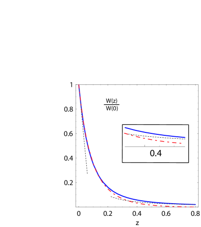
Figure 2: The dash-dotted curve corresponds to the interpolator $W[z]$ in Eq. (14), i.e. without considering the $\delta_{K}$ contribution, normalized to its value at the origin, versus $z=Q^{2}/\mu^{2}_{had}$ for $\mu_{had}=1.4$ GeV, $F_{0}=85.3$ MeV and $M_{V}=770$ MeV. The solid curve is the full function $W(z)$ in Eq. (19) after including the $\delta_{K}$ contribution in Eq. (12) (see text below). As one can see both curves are quite similar (the insert is a blow-up of the region $z\sim 0.4$). The two dashed curves correspond to the chiral and operator product expansions, for small and large values of z, respectively.

Notice that the shape of the interpolating function $W(z)$ shown in Fig. 2 is very smooth. This kind of shape for the Green’s function is very representative and we have found similar shapes in all the different cases we have studied.

One can now use the example of $W(z)$ to develop some intuition of the role played by the different energy scales in the problem. Although in a one-scale theory like QCD all scales are ultimately related to each other, it is a fact of life that there is a clear numerical hierarchy. First, there are chiral parameters such as $F_{\pi}$ or $\langle\overline{\psi}\psi\rangle^{1/3}$ whose scale is $\sim 100-200$ MeV. Second, there is a typical resonance mass, or mass gap, whose scale is much larger, i.e. $\Lambda_{QCD}\sim 1$ GeV. Notice that, since $F_{\pi}\sim N_{c}^{1/2}$ but $\Lambda_{QCD}\sim N_{c}^{0}$, a naive use of the strict large-$N_{c}$ limit would lead one to the erroneous conclusion that $\Lambda_{QCD}/F_{\pi}$ is negligible.

In matching conditions like (2.1) this observation is crucial. The reason is that the factorized contribution is governed by $F_{\pi}$ –which in Eq. (2.1) has been scaled out and this is why the first term is unity– whereas the unfactorized contribution is governed by $\Lambda_{QCD}$.

Since $W(z)\sim 1$ in the region $z\lesssim\Lambda_{QCD}^{2}/\mu_{had}^{2}$ –before the OPE sets in– and neglecting the logarithmic divergence from the OPE tail, this means that

$$\int_{0}^{\frac{\Lambda_{QCD}^{2}}{\mu_{had}^{2}}}dz\ W(z)\sim\frac{\Lambda_{QCD}^{2}}{\mu_{had}^{2}}\ ,$$ (15)

which says that the correction to unity in Eq. (2.1) will be of order $\Lambda_{QCD}^{2}/(4\pi F_{\pi})^{2}$, which is not a negligible contribution at all. In this case keeping only the factorized contribution is not safe because the $N_{c}\rightarrow\infty$ limit happens to select a scale which is “abnormally small”, $F_{\pi}$, as compared to the larger scale $\Lambda_{QCD}$, which can only show up in the next-to-leading $1/N_{c}$ terms. In these cases it is not unnatural to expect large unfactorized contributions. As a matter of fact, later on we shall see that the unfactorized contribution is $\sim 50\%$ of the factorized contribution in the case of $B_{K}$ but it is several times larger in the case of the strong penguin contribution to $\varepsilon^{\prime}/\varepsilon$.

However, once one has included the unfactorized contribution with its $\Lambda_{QCD}$ scale, there is no further scale in the game. Therefore, there is no reason to expect that subleading effects will still yield larger contributions with the consequent breakdown of the large-$N_{c}$ expansion. These subleading effects are typically either an OZI-violating amplitude or related to resonance widths, and all evidence so far is compatible with these two being reasonably small. Notice that something similar to this happens in the relationship between the $\eta^{\prime}$ mass and the topological susceptibility for different number of colors[10]: even though the $\eta^{\prime}$ mass is not at all small as compared to $\Lambda_{QCD}$ –whereas it vanishes when $N_{c}\rightarrow\infty$– the $1/N_{c}$ expansion gives a good description of the lattice data for different values of $N_{c}$, i.e. the expansion does not break down.

Let us come back to our matching condition (2.1). Having disregarded the $\delta_{K}$ contribution, one sees that the interpolator $W(z)$ in Eq. (14) crosses the OPE curve at $z\sim 0.4$ (which is equivalent to $Q\sim 900$ MeV). Merging into the OPE only takes place at values of $z$ which are larger than those shown in the plot. Assuming that the OPE is a fair description starting from $Q\sim 900$ MeV onwards, one can now get an estimate of the integral in Eq. (2.1) by first integrating with the interpolator $W(z)$ in the region $0\leq z\lesssim 0.4$ and then with the OPE curve in the region $0.4\lesssim z<\infty$. The result is usually presented in the form:

$$\widehat{B}_{K}^{\chi}=\frac{3}{4}\ \widehat{g}_{S=2}\ ,$$ (16)

and one finds $\widehat{B}_{K}^{\chi}=0.38\pm 0.11$, where the error is an estimate of higher order $1/N_{c}$ corrections, $\sim 30\%$. This error[8] covers all reasonable variations in the input parameters (e.g. the $\rho$ mass).

The combination appearing in Eq. (16) parametrizes the $K^{0}-\overline{K^{0}}$ matrix element of the $\Delta S=2$ operator in Eq. (2.1),

$$<\bar{K}^{0}|\ c(\mu)\ \left(\overline{s}_{L}\gamma^{\mu}d_{L}\right)^{2}(\mu)|K^{0}>=\frac{4}{3}F_{K}^{2}M_{K}^{2}\hat{B}_{K}\quad,$$ (17)

after including chiral corrections (this is why $\widehat{B}_{K}\neq\widehat{B}_{K}^{\chi}$), and governs quantities such as $\varepsilon_{K}$ and the $K_{L}-K_{S}$ mass difference. The inclusion of these chiral corrections is a necessary ingredient in order to make contact with the physical world since, moreover, there are indications that they may be sizeable[12]. We plan to be able to report on this in the near future but, for now, the result after Eq. (16) is still in the chiral limit.

One may now include the contribution from the $\delta_{K}$ term in the operator product expansion of Eq. (12). This coefficient $\delta_{K}$ parameterizes the following matrix element

$$<0|g_{s}\bar{s}_{L}\tilde{G}_{\mu\nu}^{a}\lambda_{a}\gamma^{\mu}d_{L}|K(p)>=-i\sqrt{2}F_{0}\ \delta_{K}^{2}\ p_{\mu}\ ,$$ (18)

and a sum rule analysis[13] gives $\delta_{K}^{2}=0.12\pm 0.07$ GeV². Since we now have one more condition at large $z$, we have to include one more resonance in the interpolator in order to achieve matching. First, we observe that the low-$z$ behavior of $W(z)$ depends on $L_{3}$ and this low-energy constant, unlike the other $L_{i}$’s appearing in (11), receives contribution from scalars resonances[14]. Second, a simple pole contribution from a scalar resonance is compatible with the analytic structure and quantum numbers shown in Fig. 1. Therefore, we enlarge the interpolator in Eq. (14) with a scalar pole to read

$$W(z)_{V,S}=\frac{a_{V}}{(z+\rho_{V})}+\frac{b_{V}}{(z+\rho_{V})^{2}}+\frac{c_{V}}{(z+\rho_{V})^{3}}+\frac{a_{S}}{(z+\rho_{S})}\quad,$$ (19)

and allow for a generous variation of the scalar resonance mass $M_{S}=900\pm 400$ MeV. Imposing that $W(z)_{V,S}$ matches both expansions in Eqs. (11, 12) one can obtain the unknown residues and determine $W(z)$, Eq. (19). This function is the solid line plotted in Fig. 2. One sees that it matches the OPE in a smoother way than the interpolator obtained earlier (dash-dotted line in Fig. 2), but there is no dramatic difference in the area underneath. In summary, the neglect of higher order terms in the expansions (11, 12), as a first approximation, is a self-consistent procedure.

Using now this improved function $W(z)$ and Eq. (2.1), we can calculate $\widehat{B}_{K}^{\chi}$ once again and obtain

$$\widehat{B}_{K}^{\chi}=0.36\pm 0.15\ ,$$ (20)

as our final value. We emphasize that, because the coupling $\widehat{g}_{S=2}$ in Eq. (5) is of $\mathcal{O}(p^{2})$ in the weak chiral Lagrangian (4), our value is in the chiral limit. This result is in nice agreement with recent determinations done on the lattice, where it now begins to be possible to consider dynamical fermions[15].

2.2 Corrections from dimension-eight quark operators.

The passage from the Lagrangian in terms of quarks and gluons (2.1) to the Lagrangian (4) in terms of Goldstone mesons requires the integration of all the resonances. But in this integration the mass scale involved is the mass gap, i.e. $\Lambda_{QCD}\sim 1$ GeV, which is not negligible compared to the charm mass. Therefore, in the matching condition for $\Lambda_{S=2}^{2}$ in Eq. (5) there may be extra contributions of $\mathcal{O}(\Lambda_{QCD}^{2})$.

To analyze the presence of these extra contributions one obviously must consider effects which are of $\mathcal{O}(\Lambda_{QCD}^{2}/m_{c}^{2})$, relative to the contributions in Eq. (5). Therefore, after integrating out the charm quark, one must go to a Lagrangian of quark operators which are dimension eight rather than dimension six as in Eq. (2.1). Since in this case there is not the competition between the scales $F_{\pi}$ and $\Lambda_{QCD}$ we discussed earlier, to simplify matters, we shall take the large-$N_{c}$ limit.

Dimensional analysis shows that $\Delta S=2$ dimension-eight operators, unlike the dimension-six operator in Eq. (2.1), cannot come with a quark mass out front. It is not surprising, then, that the GIM mechanism becomes fully operational for scales $m_{c}<\mu<m_{t},M_{W}$ while the charm quark is active, arranging combinations like $(\lambda_{c}+\lambda_{u})^{2}=\lambda_{t}^{2}$ which is numerically negligible since, unlike in the dimension-six case of Eq. (2.1), it cannot be compensated by a large $m_{t}$ factor.

At $\mu=m_{c}$, however, the charm quark is integrated out and the above mechanism no longer applies. At this scale, therefore, $\Delta S=2$ dimension-eight operators do get generated. Another simplification occurs, however. Notice that we eventually want to match onto the $\mathcal{O}(p^{2})$ chiral Lagrangian in Eq. (4). Therefore any $\Delta S=2$ operator whose matrix element between a $K^{0}$ and a $\overline{K}^{0}$ is of higher chiral order is of no interest. Furthermore, in the large-$N_{c}$ limit four quark operators factorize, i.e. they become a product of two color singlets. A dimension-eight operator can be arranged in only two ways: either as a product of two dimension-four operators, or as a product of a dimension-3 operator times a dimension-5 one. However, the first case yields contributions of higher chiral order. This is due to the fact that

$$\langle\overline{K}^{0}(p)|{\bar{s}}_{L}\gamma_{\nu}{\mathcal{D}}_{\mu}d_{L}|0\rangle\sim\left(p_{\mu}p_{\nu}-\frac{p^{2}}{4}g_{\mu\nu}\right)\ ,$$ (21)

which can be seen by contracting with $g^{\mu\nu}$ and using the equations of motion –in the chiral limit–. So, only the combination $\mathcal{O}(\mathrm{dim-3})\times\mathcal{O}(\mathrm{dim-5})$ is possible. However, $\overline{s}\widetilde{G}^{\mu\nu}\gamma_{\nu}d(x)$ is the only dimension-five current connecting a kaon to the vacuum[17]. Consequently, this means that there is only one $\Delta S=2$ dimension-eight operator to consider. This operator is given by

$$\mathcal{L}_{eff}=-\frac{G_{F}^{2}}{3\pi^{2}}\ c_{8}(\mu)\ g_{s}\overline{s}_{L}\widetilde{G}^{\mu\nu}\gamma_{\nu}d_{L}(x)\ \overline{s}_{L}\gamma_{\mu}d_{L}(x)\ +\mathrm{h.c.}\ ,$$ (22)

where $g_{s}$ is the strong coupling constant.

Integrating out the charm quark yields for the coefficient $c_{8}$ the matching condition[16]

$$c_{8}(m_{c})=-\ \frac{7}{6}\ \lambda_{u}^{2}-\frac{13}{6}\ \lambda_{c}\lambda_{u}.$$ (23)

Below the charm mass the Effective Theory is given simply by

$$\mathcal{L}_{eff}=-\frac{G_{F}^{2}}{3\pi^{2}}\ c_{8}(\mu)\ g_{s}\overline{s}_{L}\widetilde{G}^{\mu\nu}\gamma_{\nu}d_{L}\ \overline{s}_{L}\gamma_{\mu}d_{L}-\frac{G_{F}}{\sqrt{2}}\lambda_{u}\ \overline{s}_{L}\gamma^{\mu}u_{L}\ \overline{u}_{L}\gamma_{\mu}d_{L}+h.c.\ .$$ (24)

Notice that the second operator is the only one producing $\Delta S=1$ transitions in the large-$N_{c}$ limit. Away from this limit its Wilson coefficient is not unity as in Eq. (24) but gets corrected by $30\%-40\%$, as a naive estimate of typical $1/N_{c}$ corrections would say.

At scales $\mu\lesssim m_{c}$, while one can still consider QCD in the perturbative regime, the Wilson coefficient $c_{8}(\mu)$ runs due to the fact that the square of the $\Delta S=1$ operator in Eq. (24), with the two up-quarks propagating in a loop, mixes into the direct $\Delta S=2$ operator. At lowest order in the strong coupling constant, which is enough for our purposes, one finds[16] for scales $\mu\sim\Lambda_{QCD}\sim 1$ GeV,

$$c_{8}(\mu)=c_{8}(m_{c})+\lambda_{u}^{2}\log\frac{\mu^{2}}{m_{c}^{2}}\ ,$$ (25)

where $c_{8}(m_{c})$ is given by Eq. (23).

At scales $\mu\sim M_{K}\ll\Lambda_{QCD}$ perturbation theory is no longer a valid approximation and the matching of the Lagrangian (24) to the chiral Lagrangian (4) requires again the machinery of the Hadronic Approximation to large-$N_{c}$ we used in the previous section. Skipping the details of this calculation[16], we find that the coupling constant $\Lambda^{2}_{S=2}$ gets the following contribution,

$$\Lambda^{2}_{S=2}|_{\mathrm{dim-8}}=\left\{\frac{26}{9}\ \lambda_{c}\lambda_{u}\ \delta_{K}^{2}+\lambda_{u}^{2}\ (0.95\ \mathrm{GeV})^{2}\right\}\left(1\pm 0.3\right)\ ,$$ (26)

where $\delta_{K}^{2}$ is the parameter defined in Eq. (18), and the error is an estimate of the size of a typical $1/N_{c}$ correction. Notice that all renormalization scale and scheme dependence has canceled out, as it should. This is one of the advantages of using the HA framework.

The first contribution in (26) bears the mark of charm in $\lambda_{c}$ and stems from the matching condition for the Wilson coefficient $c_{8}(m_{c})$ when charm gets integrated out. Although it has an imaginary part that contributes to $\varepsilon_{K}$, its size is governed by the dynamical scale $\delta_{K}\sim 350$ MeV, which is small enough relative to $m_{c}$ to yield a very small correction to $\varepsilon_{K}$.

The second contribution is the result of the running below the charm mass and subsequent matching onto the chiral Lagrangian (4); this is where resonances get integrated out. This is why only $\lambda_{u}$ appears and, also, why the energy scale, which is a combination of resonance masses and couplings, is essentially given by the mass gap $\Lambda_{QCD}\sim 1$ GeV. Since $\lambda_{u}$ is purely real it cannot contribute to $\varepsilon_{K}$. The energy scale in (26) is comparable to $m_{c}$, which explains why the $K_{L}-K_{S}$ mass difference gets a sizeable $\sim 10-20\%$ correction[16].

3 $\varepsilon^{\prime}/\varepsilon$ and the $\Delta I=1/2$ rule: “penguinology”.

At scales $\mu\lesssim m_{c}$ the Standard Model gives rise to 10 four-quark operators capable of producing $\Delta S=1$ transitions[1]. All these operators mix as the renormalization scale evolves.

On the other hand, at the scale of the Kaon, the Effective Field Theory for $\Delta S=1$ transitions is described by the chiral Lagrangian[5]

$$\!\mathcal{L}_{eff}^{\Delta S=1}=-\frac{G_{F}}{\sqrt{2}}\ V_{ud}V_{us}^{*}\left\{g_{8}\mathcal{L}_{8}+g_{27}\mathcal{L}_{27}+e^{2}g_{ew}\mathrm{Tr}\left(U\lambda_{L}^{(32)}U^{{\dagger}}Q_{R}\right)\right\}\,,$$ (27)

where

$$\mathcal{L}_{8}=\sum_{i=1,2,3}(\mathcal{L}_{\mu})_{2i}\ (\mathcal{L}^{\mu})_{i3}\quad,\quad\mathcal{L}_{27}=\frac{2}{3}(\mathcal{L}_{\mu})_{21}\ (\mathcal{L}^{\mu})_{13}+(\mathcal{L}_{\mu})_{23}\ (\mathcal{L}^{\mu})_{11}\,,$$

with $\mathcal{L}_{\mu}=-iF_{0}^{2}\ U(x)^{\dagger}D_{\mu}U(x)$ , $\lambda_{L}^{(32)}=\delta_{i3}\delta_{j2}$ and $Q_{L,R}=\mathrm{diag}(2/3,-1/3,-1/3)$.

In this section we shall concentrate on the contribution to $\varepsilon^{\prime}/\varepsilon$ from $Q_{6}$ which, together with the one from $Q_{8}$[27, 28], is the dominant one[29]. As we shall see, the analysis will tell us interesting things about the $\Delta I=1/2$ rule as well.

We may now run the Effective Field Theory from $M_{W}$ down to the charm mass as usual but, at this point, make some simplifications in the analysis not to have to deal with the full $10\times 10$ operator mixing matrix. Our first simplification will be to stay within the leading-log approximation. Furthermore we shall go to first subleading order in the $1/N_{c}$ expansion but keeping only those terms which are enhanced by an extra factor of $n_{F}$, the number of flavors. In this case, the operator $Q_{6}$ only mixes with $Q_{4}$, where

$$Q_{6}=-8\sum_{q=u,d,s}\left(\overline{s}_{L}q_{R}\right)\left(\overline{q}_{R}d_{L}\right)\quad,\quad Q_{4}=4\sum_{q=u,d,s}\left(\overline{s}_{L}\gamma^{\mu}q_{L}\right)\left(\overline{q}_{L}\gamma_{\mu}d_{L}\right)\ ,\$$ (28)

and the sum over color indices within brackets is understood.

The matching condition then reads[18]

$$g_{8}(Q_{4},Q_{6})\!\! = \!c_{6}(\mu)\Bigg{\{}\frac{-16L_{5}(\mu)\langle\overline{\psi}\psi\rangle^{2}(\mu)}{F_{0}^{6}}+\frac{8n_{f}}{16\pi^{2}F_{0}^{4}}\!\!\int_{0}^{\infty}\!\!\!\!\!dQ^{2}Q^{2}\mathcal{W}_{DGRR}(Q^{2})\Bigg{\}}_{\!\!\!\overline{\mathrm{MS}}}$$ (29)

$$+ c_{4}(\mu)\ \Bigg{\{}1-\frac{4n_{f}}{16\pi^{2}F_{0}^{4}}\int_{0}^{\infty}\!\!\!\!\!dQ^{2}Q^{2}\ \mathcal{W}_{LLRR}(Q^{2})\Bigg{\}}_{\overline{\mathrm{MS}}}\ .$$

In the previous expression the subscript $\overline{\mathrm{MS}}$ is a reminder that these integrals are UV divergent and have to be regularized and renormalized using the same scheme as for the Wilson coefficients $c_{4,6}$. This is also true for $\langle\overline{\psi}\psi\rangle$ and $L_{5}$. As far as the $N_{c}$ counting goes, all the unfactorized contributions, which are of $\mathcal{O}(n_{F}/N_{c})$, are contained in the terms proportional to the functions $\mathcal{W}_{DGRR}$ and $\mathcal{W}_{LLRR}$. The terms proportional to $L_{5}$ and unity correspond to the factorized contribution from $Q_{6}$ and $Q_{4}$ –respectively– and, formally, are of $\mathcal{O}(N_{c}^{0})$.

The functions $\mathcal{W}_{DGRR}$ and $\mathcal{W}_{LLRR}$ are defined through the connected four-point Green’s functions

$$\!\!\!\!\!\!\!\!\!\!\!\!\!\!\!\!\mathcal{W}_{DGRR}^{~{}~{}~{}~{}\alpha\beta}(q)=i^{3}\!\!\!\int\!\!d^{4}x\ d^{4}y\ d^{4}z\ e^{iq.x}\langle T\{D_{\bar{s}q}(x)G_{\bar{q}d}(0)R_{\bar{d}u}^{\alpha}(y)R_{\bar{u}s}^{\beta}(z)\}\rangle\ ,$$

$$\!\!\!\!\!\!\!\!\!\!\!\!\!\!\!\mathcal{W}_{LLRR}^{\,\mu\,\mu\,\alpha\,\beta}(q)=i^{3}\!\!\!\int\!\!d^{4}x\ d^{4}y\ d^{4}z\ e^{iq\cdot x}\langle T\{L_{\bar{s}q}^{\mu}(x)L^{\bar{q}d}_{\mu}(0)R_{\bar{d}u}^{\alpha}(y)R_{\bar{u}s}^{\beta}(z)\}\rangle\ ,$$ (30)

after integration over the solid angle in $q$-momentum space, as in Eq. (8). In these expressions $D_{\bar{s}q}=\overline{s}_{L}q_{R},\ G_{\bar{q}d}=\overline{q}_{R}d_{L},\ L_{\bar{s}q}^{\mu}=\overline{s}_{L}\gamma^{\mu}q_{L},\ R_{\bar{d}u}^{\alpha}=\overline{d}_{R}\gamma^{\alpha}u_{R}$, etc. It is not a coincidence that the pair of fermion bilinears which make up the operators $Q_{6,4}$ in Eq. (28) also appear in these Green’s functions, although they are located at different space-time points. It is the integral over $Q$ in Eq. (29) which puts these two points back on top of each other. The matching condition (29) imposes that the same “mass term” $r_{\overline{d}u}^{\alpha}r^{\overline{u}s}_{\alpha}$ is obtained when computed from the covariant derivatives in the Chiral Lagrangian (27) –which yields directly $g_{8}$– as when computed from the four-quark Effective Lagrangian, which requires the insertion of the combination $c_{6}Q_{6}+c_{4}Q_{4}$ in the form shown in Eq. (29).

In order to calculate the unfactorized contribution one should now construct the Hadronic Approximation. As in the previous case of $B_{K}$, an explicit cancelation of the renormalization scale dependence is achieved. This is good news since the scale dependence of the factorized contribution is very large: it changes by a factor $\sim 2$ if the renormalization scale is varied in the range $M_{\rho}\leq\mu\leq 1$ GeV. Since this dependence has to be canceled by the unfactorized contributions, it is not unthinkable that these contributions be large. As discussed in the previous section on more general grounds, this could even be expected.

And, indeed, it was found[18] that the unfactorized contribution from the operator $Q_{6}$ to the coupling $g_{8}$ in the matching condition (29) was a factor $\sim 3$ larger than the factorized contribution at a scale $\mu=0.8$ GeV. Although the effect was somewhat smaller for $Q_{4}$, an enhancement was found there as well. Both large contributions come from what in the jargon is called an “eye” diagram (i.e. the contraction of the “dummy” quark $q$ in the sums in Eq. (28)). On the basis of a Nambu-Jona-Lasinio model, this enhancement has also been found by Bijnens and Prades[20].

Decomposing the Wilson coefficients as[1]

$$c_{i}(\mu)\!=z_{i}(\mu)+\tau y_{i}(\mu)\quad,\quad\tau\!=-\frac{V^{*}_{ts}V_{td}}{V^{*}_{us}V_{ud}}\ ,$$ (31)

the imaginary part of the coupling constant $g_{8}$ in Eq. (29) becomes

$$\mathrm{Im}g_{\underline{8}}\simeq(3\pm 1)\times\mathrm{Im}\tau\ ,$$ (32)

where the error is the result of varying the quark condensate (which is the source of the biggest uncertainty), in the range $\langle\overline{\psi}\psi\rangle^{1/3}(2\ \mathrm{GeV})=(0.240-0.260)$ GeV. As to $\mathrm{Im}\tau$, its current value[23] is $-6.0(5)\times 10^{-4}$.

We can also estimate $\mathrm{Re}g_{8}$ and $g_{27}$. This is a very tough test for any calculational framework, as it is in these parameters that the $\Delta I=1/2$ rule is rooted; a rule which still to this date defies detailed understanding. However, at the scale $\mu=m_{c}$, the situation is particularly simple since only the operators

$$Q_{2}=4(\bar{s}_{L}\gamma^{\mu}u_{L})(\bar{u}_{L}\gamma_{\mu}d_{L})\quad,\quad Q_{1}=4(\bar{s}_{L}\gamma^{\mu}d_{L})(\bar{u}_{L}\gamma_{\mu}u_{L})\$$ (33)

have nonvanishing real Wilson coefficients. Although at scales $\mu\ll m_{c}$ penguin operators will again come into play, it is not crazy to neglect this effect and stay “as if $\mu=m_{c}$” in a first approximation. In this case the contribution to $\mathrm{Re}g_{8}$ from $Q_{1,2}$ can be estimated because the non-eye diagrams are related to those appearing in the matching condition for $\widehat{g}_{S=2}$ in the case of $B_{K}$,[25] while the eye diagram of $Q_{2}$ can be estimated from the eye diagram of $Q_{4}$ in the matching condition (29), just setting $n_{F}=1$. In numbers this leads to[18] $\mathrm{Re}g_{8}=2.1\pm 0.8$, to be compared to the experimental result[21, 24] $\mathrm{Re}g_{8}=3.6\pm 0.1$, after subtraction of chiral corrections. In spite of the large errors involved I find this result quite encouraging, mainly because the strict large-$N_{c}$ result (factorization) would lead to $\mathrm{Re}g_{8}=0.6$ which is way too small. We begin to see the large unfactorized contributions which are indispensable for understanding the $\Delta I=1/2$ rule although, clearly, a more detailed analysis is needed before victory can be claimed.

$SU(3)$ allows to relate $\widehat{g}_{S=2}$ in $B_{K}$ to $g_{27}$ because their corresponding matching conditions to the four-quark Lagrangian are $SU(3)$ rotations of each other[26]. This leads to $g_{27}=\widehat{g}_{S=2}=0.27\pm 0.12$, to be compared to $g_{27}=0.30\pm 0.01$ as extracted from experiment[21, 24].

Using all these results, together with[27, 28]

$$\mathrm{Im}\left(e^{2}g_{ew}\right)=(1.6\pm 0.4)\cdot 10^{-6}\ \mathrm{GeV}^{6}\times\mathrm{Im}\tau\ ,$$ (34)

and, including final state interactions[30] and isospin breaking effects[21], one obtains[18] $\varepsilon^{\prime}/\varepsilon=(5\pm 3)\times 10^{-3}$ to be compared to the experimental number[22] $(1.66\pm 0.16)\times 10^{-3}$. This is not a bad result considering our approximations.

4 Application to lattice QCD: quenching penguins.

Current calculations of $\varepsilon^{\prime}/\varepsilon$ done on the lattice require getting rid of the fermion determinant in the path integral in order to be numerically efficient. This is accomplished by introducing some ghosts quarks which, although spin 1/2 particles, commute. This lattice technique, known as “quenching”, has some dramatic consequences. In particular the flavor symmetry group is changed from the usual $SU(3)_{L}\times SU(3)_{R}$ to a graded $SU(3|3)_{L}\times SU(3|3)_{R}$[31]. Furthermore, and even more importantly, there is no reason for the quenched theory to have the same weak low-energy constants as the true theory. The fact is that the current result for $\varepsilon^{\prime}/\varepsilon$ on the lattice is 3 times smaller than the experimental result, and with the opposite sign[32].

A particularly clear example of this is the transformation undergone by the strong penguin operator $Q_{6}$ in the quenched theory[33]. After quenching, the operator $Q_{6}$ in Eq. (28) is no longer a singlet under $SU(3)_{R}$, or rather under $SU(3|3)_{R}$. Instead, it can be decomposed as

$$Q_{6}=\underbrace{2(\overline{s}_{L}^{\alpha}\gamma_{\mu}d_{L}^{\beta})(\overline{q}_{R}^{\beta}\gamma^{\mu}q_{R}^{\alpha}+\overline{\widetilde{q}}_{R}^{\beta}\gamma^{\mu}\widetilde{q}_{R}^{\alpha})}_{\frac{1}{2}Q_{6}^{QS}}+\underbrace{2(\overline{s}_{L}^{\alpha}\gamma_{\mu}d_{L}^{\beta})(\overline{q}_{R}^{\beta}\gamma^{\mu}q_{R}^{\alpha}-\overline{\widetilde{q}}_{R}^{\beta}\gamma^{\mu}\widetilde{q}_{R}^{\alpha})}_{Q_{6}^{QNS}}$$ (35)

where the tilde on top refers to the ghost quarks. The flavor properties are such that $\mathcal{Q}_{6}^{QS}$ is a singlet under the quenched flavor group $SU(3|3)_{R}$ whereas $\mathcal{Q}_{6}^{QNS}$ is not. This changes their chiral representation accordingly[33]:

$$\mathcal{Q}_{6}^{QS} \Rightarrow -\ \alpha^{(8,1)}_{q1}\ \mathrm{STr}\left(\Lambda\mathcal{L}_{\mu}\mathcal{L}^{\mu}\right)+\ \alpha^{(8,1)}_{q2}\ \mathrm{STr}\left(2B_{0}\Lambda(UM+MU^{\dagger})\right)\qquad$$

$$\mathcal{Q}_{6}^{QNS} \Rightarrow f^{2}\alpha^{NS}_{q}\ \mathrm{STr}\left(\Lambda U\widehat{N}U^{\dagger}\right)\ ;\ \widehat{N}=\frac{1}{2}\,{\rm diag}\left(1,1,1,-1,-1,-1\right)\qquad$$ (36)

with $\overline{q}\Lambda q=\overline{s}d$, $M$ the quark-mass matrix, and $\mathrm{STr}$ is the so-called supertrace. $\widehat{N}$ exhibits the non-singlet structure of $\mathcal{Q}_{6}^{QNS}$. Comparing Eqs. (27) and (4), one sees that the couplings $\alpha^{(8,1)}_{q1,2}$ have a counterpart in the true theory (the weak mass term of $\alpha^{(8,1)}_{q2}$ is not written in Eq. (27)), but $\alpha^{NS}_{q}$ is a total quenching artifact.

As we did in previous sections, it is now straightforward to apply large $N_{c}$ to determine these coupling constants $\alpha^{(8,1)}_{q1},\ \alpha^{NS}_{q}$. One conclusion follows immediately: because of the presence of the degenerate ghosts quarks, the sum over flavor in the internal propagator of the eye diagrams exactly vanishes. But this contribution was actually the dominant one in the QCD case!. Thus one obtains[34]:

• the contribution from $Q_{6}$ to $\alpha^{(8,1)}_{q1}$ is much smaller than its counterpart in the true theory, $g_{8}$; and,

• $\frac{\alpha_{q}^{NS}}{\alpha_{q1}^{(8,1)}}=\frac{1}{16L_{5}}\simeq 60\$,

where the quenched result[35] $L_{5}\simeq 10^{-3}$ has been used. A recent lattice analysis[36] has obtained

$$\frac{\alpha_{q}^{NS}}{\alpha_{q1}^{(8,1)}}=57(13)\ ,$$ (37)

in nice agreement with our prediction (not postdiction!) above.

5 Conclusions.

Nature has an approximate chiral symmetry because the $u,d,s$ quark masses are small. On a lattice, Nature is approached from the side of heavy quark masses by using chiral symmetry to guide the extrapolation. However, chiral symmetry is a property which is very difficult to achieve on the lattice, taking long hours of calculations with sophisticated codes and expensive computers and, regretfully, this becomes an important source of error.

Large-$N_{c}$ QCD offers the possibility to approach the problem from the other end. In the continuum chiral symmetry is much easier to achieve: it only takes the time needed to write a chiral Lagrangian. Furthermore, analytic calculations yield an understanding of the problem which allows building physical intuition. However, the flip side is that chiral symmetry is only exact when the quark masses are zero. To get to the real world, one must work one’s way up to realistic quark masses by computing chiral corrections.

I hope that the work presented here shows, among other things, how the continuum large-$N_{c}$ expansion may complement the lattice approach towards understanding kaon weak interactions.

References

- [1] A. J. Buras et al. Nucl. Phys. B 370 (1992) 69 [Addendum-ibid. B 375 (1992) 501]; M. Ciuchini et al. Nucl. Phys. B 415 (1994) 403 [arXiv:hep-ph/9304257]. For a review see, A. J. Buras, arXiv:hep-ph/9806471;
- [2] G. ’t Hooft, Nucl. Phys. B 72 (1974) 461; E. Witten, Nucl. Phys. B 160 (1979) 57. For a review, see A. V. Manohar, arXiv:hep-ph/9802419.
- [3] S. Peris, arXiv:hep-ph/0204181; E. de Rafael, Nucl. Phys. Proc. Suppl. 119, 71 (2003) [arXiv:hep-ph/0210317].
- [4] See, e.g., A. J. Buras, arXiv:hep-ph/0307203.
- [5] See the reviews in, e.g., E. de Rafael, arXiv:hep-ph/9502254, A. Pich, arXiv:hep-ph/9806303. J. Bijnens, arXiv:hep-ph/0204068.
- [6] C. Bender and S. Orszag, “Advanced Mathematical Methods for Scientists and Engineers I: asymptotic methods and perturbation theory”, Springer 1999; section 8.5.
- [7] M. Golterman et al. JHEP 0201 (2002) 024 [arXiv:hep-ph/0112042].
- [8] S. Peris et al. Phys. Lett. B 490 (2000) 213 [arXiv:hep-ph/0006146 v3] (See erratum in e-preprint); S. Peris, Nucl. Phys. Proc. Suppl. 96 (2001) 346 [arXiv:hep-ph/0010162].
- [9] H. Jeffreys and B. Swirles, “Methods of Mathematical Physics”, Cambridge Univ. Press, 1956, section 12.06.
- [10] B. Lucini et al. JHEP 0106 (2001) 050 [arXiv:hep-lat/0103027].; B. Lucini et al. arXiv:hep-lat/0309170.
- [11] J. Bijnens et al. JHEP 9901 (1999) 023 [arXiv:hep-ph/9811472].
- [12] J. Bijnens et al. JHEP 0001 (2000) 002 [arXiv:hep-ph/9911392]. S. Hashimoto, arXiv:hep-ph/0411126, and references therein.
- [13] O. Cata et al. JHEP 0303 (2003) 060 [arXiv:hep-ph/0303162].
- [14] G. Ecker et al. Nucl. Phys. B 321 (1989) 311; G. Ecker et al. Phys. Lett. B 223 (1989) 425. J. Bijnens et al. Mod. Phys. Lett. A 11 (1996) 1069 [arXiv:hep-ph/9510338]. S. Peris et al. JHEP 9805 (1998) 011 [arXiv:hep-ph/9805442]. A. Pich, arXiv:hep-ph/0205030.
- [15] Y. Aoki et al. arXiv:hep-lat/0411006 and references therein.
- [16] O. Cata et al. JHEP 0407 (2004) 079 [arXiv:hep-ph/0406094].
- [17] V. A. Novikov et al. Nucl. Phys. B 237 (1984) 525.
- [18] T. Hambye et al. JHEP 0305 (2003) 027 [arXiv:hep-ph/0305104]; S. Peris, arXiv:hep-ph/0310063.
- [19] E. Pallante et al. Nucl. Phys. B 617 (2001) 441 [arXiv:hep-ph/0105011].
- [20] J. Bijnens et al. JHEP 0006 (2000) 035 [arXiv:hep-ph/0005189]. See however, S. Peris et al. JHEP 9805 (1998) 011 [arXiv:hep-ph/9805442].
- [21] V. Cirigliano et al. Eur. Phys. J. C 33 (2004) 369 [arXiv:hep-ph/0310351].
- [22] A. Alavi-Harati et al. [KTeV Collaboration], Phys. Rev. D 67 (2003) 012005 [arXiv:hep-ex/0208007]; J. R. Batley et al. [NA48 Collaboration], Phys. Lett. B 544 (2002) 97 [arXiv:hep-ex/0208009].
- [23] A. J. Buras, arXiv:hep-ph/0307203.
- [24] J. Bijnens et al. Nucl. Phys. B 648 (2003) 317 [arXiv:hep-ph/0205341].
- [25] A. Pich et al. Phys. Lett. B 374 (1996) 186 [arXiv:hep-ph/9511465].
- [26] J. F. Donoghue et al. Phys. Lett. B 119 (1982) 412.
- [27] M. Knecht et al. Phys. Lett. B 508 (2001) 117 [arXiv:hep-ph/0102017]; M. Knecht et al. Phys. Lett. B 457 (1999) 227 [arXiv:hep-ph/9812471]. S. Friot et al. JHEP 0410 (2004) 043 [arXiv:hep-ph/0408281].
- [28] J. Bijnens et al. JHEP 0110 (2001) 009 [arXiv:hep-ph/0108240]. V. Cirigliano et al. Phys. Lett. B 555 (2003) 71 [arXiv:hep-ph/0211420]. S. Narison, Nucl. Phys. B 593 (2001) 3 [arXiv:hep-ph/0004247]. T. Blum et al. [RBC Collaboration], Phys. Rev. D 68 (2003) 114506 [arXiv:hep-lat/0110075]. J. I. Noaki et al. [CP-PACS Collaboration], Phys. Rev. D 68 (2003) 014501 [arXiv:hep-lat/0108013]. A. Donini et al. Phys. Lett. B 470 (1999) 233 [arXiv:hep-lat/9910017]. T. Bhattacharya et al. Nucl. Phys. Proc. Suppl. 106 (2002) 311 [arXiv:hep-lat/0111004]. D. Becirevic et al. [SPQCDR Collaboration], Nucl. Phys. Proc. Suppl. 119 (2003) 359 [arXiv:hep-lat/0209136].
- [29] A. J. Buras et al. JHEP 0401 (2004) 048 [arXiv:hep-ph/0306217].
- [30] E. Pallante et al. Nucl. Phys. B 617 (2001) 441 [arXiv:hep-ph/0105011].
- [31] C. W. Bernard et al. Phys. Rev. D 46 (1992) 853 [arXiv:hep-lat/9204007].
- [32] T. Blum et al. [RBC Collaboration], Phys. Rev. D 68 (2003) 114506 [arXiv:hep-lat/0110075]. J. I. Noaki et al. [CP-PACS Collaboration], Phys. Rev. D 68 (2003) 014501 [arXiv:hep-lat/0108013].
- [33] M. Golterman et al. JHEP 0110 (2001) 037 [arXiv:hep-lat/0108010].
- [34] M. Golterman et al. Phys. Rev. D 68 (2003) 094506 [arXiv:hep-lat/0306028]; M. Golterman et al. Nucl. Phys. Proc. Suppl. 129 (2004) 311 [arXiv:hep-lat/0309101].
- [35] J. Heitger et al. [ALPHA Collaboration], Nucl. Phys. B 588 (2000) 377 [arXiv:hep-lat/0006026]. W. A. Bardeenet al. Nucl. Phys. Proc. Suppl. 119 (2003) 242 [arXiv:hep-lat/0209164].
- [36] J. Laiho, arXiv:hep-lat/0409113. See also talk delivered at the workshop, “Matching light quarks to Hadrons”, Benasque (Spain), http://benasque.ecm.ub.es/benasque/2004quarks/2004quarks-talks/laiho.pdf