Abstract

In many SUSY models the first SUSY signal in the proposed International Linear Collider is expected to come from the pair production of $\tilde{\tau}_{1}$, followed by its decay into $\tau+$ LSP. We study a simple and robust method of measuring the polarization of this $\tau$ in its 1-prong hadronic decay channel, and show how it can be used to discriminate between SUSY models and to determine SUSY parameters.

Introduction

It is widely recognized now that the LHC should provide unambiguous signals of supersymmetry; but one needs the data from the proposed International Linear Collider(ILC) to discriminate between different SUSY models as well as for model independent determination of the SUSY parameters [1]. One expects the lighter tau slepton,

$$\tilde{\tau}_{1}=\tilde{\tau}_{R}\sin\theta_{\tau}+\tau_{L}\cos\theta_{\tau},$$ (1)

to play a very important role in the SUSY study at ILC, since it is expected to be the lightest sfermion and the next to lightest superparticles (NLSP) over a large range of SUSY parameters in many important versions of the MSSM [2, 3]. Consequently the first SUSY signal at ILC is expected to come from the pair production of $\tilde{\tau}_{1}$.

In the universal SUGRA model the superparticle masses at the weak scale are related to the universal SUSY breaking mass parameters at the GUT scale, $m_{0}$ and $m_{1/2}$, by the renormalization group equations(RGE). The lighter neutralinos($\tilde{Z}_{1,2}$) and chargino state($\tilde{W}_{1}$) are dominated by the U(1) and SU(2) gauginos, $\tilde{B}$ and $\tilde{W}$, with masses

$$M_{1}=\frac{5\alpha_{1}}{3\alpha_{2}}M_{2}\simeq 0.5M_{2},$$

$$M_{2}=\frac{\alpha_{2}}{\alpha_{G}}m_{1/2}\simeq 0.8m_{1/2}.$$ (2)

The left and right slepton masses are given by

$$m_{\tilde{l}_{L}}^{2}=m_{0}^{2}+0.5m_{1/2}^{2},$$

$$m_{\tilde{l}_{R}}^{2}=m_{0}^{2}+0.15m_{1/2}^{2}.$$ (3)

At moderate to large $\tan\beta$($\geq 5$) the ${\tilde{\tau}}_{L,R}$ masses are suppressed by negative contributions to the above RGE from the $\tau$ yukawa coupling,

$$h_{\tau}^{2}=\frac{g^{2}m_{\tau}^{2}}{2m_{W}^{2}\cos^{2}\beta}$$ (4)

which is twice as large in $\tilde{\tau}_{R}$ as in $\tilde{\tau}_{L}$. Moreover there is significant mixing between the $\tilde{\tau}_{L,R}$ states, as represented by the off-diagonal term in the mass matrix

$$m^{2}_{LR}=-m_{\tau}(A_{\tau}+\mu\tan\beta)$$ (5)

which suppresses the mass of the lighter eigenstate $\tilde{\tau}_{1}$ further down. Thus $\tilde{\tau}_{1}$ is predicted to be the lightest sfermion over the moderate to large $\tan\beta$($\geq$ 5) region, which is favored by the LEP limit on the light Higgs boson mass. Moreover from eqs. 2-5 one expects $\tilde{\tau}_{1}$ to be the NLSP after $\tilde{Z}_{1}$, over half the parameter space

$$m_{0}<m_{1/2}.$$ (6)

The RGE of eqs.2 and  3 may not hold in non-universal versions of SUGRA and the gauge or anomaly mediated supersymmetry breaking models (GMSB and AMSB). Nonethless the suppressions coming from the Yukawa coupling and the off-diagonal mass term of eqs. 4 and  5 continue to hold in these models for moderate to large values of $\tan\beta$. Consequently the $\tilde{\tau}_{1}$ is expected to be the NLSP over important ranges of parameter space in these models as well. For simplicity we shall consider the CP conserving versions of these models.

The superparticle spectrum for a set of benchmark points for the above mentioned SUSY models, called the Snowmass points and slopes(SPS), are given in Ref. [5]. They satisfy all the experimental constraints including the cosmological constraint on the SUSY dark matter (DM) relic density. Three of the five universal SUGRA points have $\tilde{\tau}_{1}$ as the NLSP, including the typical SUGRA points(SPS1). The two exceptions represent the focus point region $m_{0}\gg m_{1/2}$ and the so called funnel region($\tan\beta=55$ and $m_{0}>m_{1/2}$). The DM constraint is satisfied through the pair annihilation of $\tilde{Z}_{1}$ by their coupling to the Z boson via their higgsino components in the focus point region and by their coupling to the pseudoscalar Higgs boson in the funnel region. In the other cases it is satisfied through the pair annihilation of $\tilde{Z}_{1}$ via a relatively light $\tilde{\tau}_{1}$ exchange $\tilde{Z}_{1}\tilde{Z}_{1}\rightarrow\tau^{+}\tau^{-}$ or its co-annihilation with a nearly dengenerate $\tilde{\tau}_{1}$. The list contains a non-universal SUGRA point(SPS6), where the $\tilde{Z}_{1}$ has a significant higgsino component and a roughly similar mass as $\tilde{Z}_{2}$ and $\tilde{W}_{1}$. In this case $\tilde{\tau}_{1}$ is slightly heavier than this cluster. It should be added here that specific non-universal SUGRA models have been considered, where the gaugino masses arise from the vacuum expectation value(vev) of a non-singlet chiral superfield, belonging to the 75 or 200 representations of the GUT SU(5) group [6]. In these models the LSP consists of a set of degenerate higgsino $\tilde{Z}_{1,2}$ and $\tilde{W}_{1}$. The $\tilde{\tau}_{1}$ turns out to be the next heavier state over the region(6) for moderate to large $\tan\beta$. The list of Ref.[5] contains two GMSB points, where the $\tilde{\tau}_{1}$ is the NLSP to a very light gravitino $\tilde{G}$ in one case and it is slightly heavier than the $\tilde{Z}_{1}$ in the other. Finally it contains a AMSB point, where the $\tilde{\tau}_{1}$ is the NLSP to a degenerate pair of $\tilde{Z}_{1},\tilde{W}_{1}$ LSP, representing the $\tilde{W}$.

One sees from the above discussion that the $\tilde{\tau}_{1}$ is expected to be the NLSP in a wide class of SUSY models. Thus one expects an unambiguous SUSY signal from the pair production process

$$e^{+}e^{-}\rightarrow\tilde{\tau}^{+}_{1}\tilde{\tau}^{-}_{1},$$ (7)

followed by the decays

$$\tilde{\tau}^{\pm}_{1}\rightarrow\tau^{\pm}\tilde{Z}_{1}.$$ (8)

In particular one can have a right polarized electron beam $(P_{e}=+1)$, which couples only to the $U(1)_{Y}$ gauge boson $B$. Thus for $s\gg m^{2}_{Z}$, $\sigma(\tilde{\tau}_{R})=4\sigma(\tilde{\tau}_{L})$; so that one can predict the $\tilde{\tau}_{1}$ pair production cross section in terms of its mass and mixing angle [7, 8]. The mass can be estimated from a threshold scan and the mixing angle from the production cross section. Hence one can then predict the polarization of $\tau$ coming from the decay (8) in terms of the composition of the LSP, i.e.

$$P_{\tau} = {\left(a^{R}_{11}\right)^{2}-\left(a^{L}_{11}\right)^{2}\over\left(a^{R}_{11}\right)^{2}+\left(a^{L}_{11}\right)^{2}},$$

$$a^{R}_{11} = -{2g\over\sqrt{2}}N_{11}\tan\theta_{W}\sin\theta_{\tau}-{gm_{\tau}\over\sqrt{2}m_{W}\cos\beta}N_{13}\cos\theta_{\tau},$$

$$a^{L}_{11} = {g\over\sqrt{2}}\left[N_{12}+N_{11}\tan\theta_{W}\right]\cos\theta_{\tau}-{gm_{\tau}\over\sqrt{2}m_{W}\cos\beta}N_{13}\sin\theta_{\tau},$$ (9)

where

$$\tilde{Z}_{1}=N_{11}\tilde{B}+N_{12}\tilde{W}+N_{13}\tilde{H}_{1}+N_{14}\tilde{H}_{2},$$ (10)

and we have made the collinear approximation($m_{\tau}\ll m_{\tilde{\tau}_{1}}$).

In this work we investigate the prospect of using $\tau$ polarization to probe the composition of $\tilde{Z}_{1}$ at the ILC. We shall use a simple and powerful method of measuring $\tau$ polarization via its inclusive 1-prong hadronic decay, which was suggested in  [9, 10] in the context of charged Higgs boson signal. The efficacy of this method for $H^{\pm}$ search has been corroborated by detailed simulation studies by both the CMS and ATLAS groups at LHC [11]. More recently the method has been used in the context of the $\tilde{\tau}_{1}$ signature at Tevatron and LHC [12]. However this seems to us to be the first application of this method for a $e^{+}e^{-}$ collider signal. It should be noted here that some of the $\tilde{\tau}$ signal studies at $e^{+}e^{-}$ collider have used the effect of $\tau$ polarization in its exclusive decay channels $\tau\to\pi\nu$ [7, 8] and $\tau\to\rho\nu$ [7]. This has its own advantage if one wants e.g. to reconstruct the $\tilde{\tau}$ mass from its decay kinematics rather than via threshold scan. But as a method of simply measuring the $\tau$ polarization the inclusive channel has several advantages over the exclusive ones, since the latter suffers from lower statistics due to the branching fraction of the particular exclusive channel as well as larger systematic error due to the contaminations from the other decay channels. The estimation of this systematic error depends heavily on the ILC detector parameters, which is beyond the scope of this paper. We can only refer the interested reader to the paper of Nojiri et. al. [7] who have done a Monte Carlo simulation incorporating the parameters of a specific model detector. In particular one can see from their fig.7 a significant contamination of the $\tau\rightarrow\rho\nu$ decay channel from $\tau\rightarrow a_{1}\nu$. On the other hand the method advocated here uses a feature of $\tau$ polarization, to which the $\pi$, $\rho$ and $a_{1}$ decay channels contribute coherently. This obviates the necessity to separate these exclusive decay channels from one another as we see below. In view of the expected improvements in a future ILC detector, it is quite possible that the systematic errors in the exclusive analysis will be reduced. In such a situation, the information obtained from both the inclusive and the exclusive analysis, can be used effectively together.

 $\tau$ Polarization

The hadronic decay channel of $\tau$ is known to be sensitive to $\tau$ polarization [9, 10]. We shall concentrate on the 1-prong hadronic decay of $\tau$, which is best suited for $\tau$ identification [11]. It accounts for 80% of $\tau$ hadronic decay and 50% of its total decay width. The main contributors to the 1-prong hadronic decay are [3],

$$\tau^{\pm}\rightarrow\pi^{\pm}\nu(12.5\%),\ \rho^{\pm}\nu(26\%),\ a^{\pm}_{1}\nu(7.5\%),$$

where the branching fractions for $\pi$ and $\rho$ include the small $K$ and $K^{\star}$ contributions respectively, which have identical polarization effects. Together they account for 90% of the 1-prong hadronic decay. The CM angular distribution of $\tau$ decay into $\pi$ or a vector meson $v(=\rho,a_{1})$ is simply related to its polarization via

$${1\over\Gamma_{\pi}}{d\Gamma_{\pi}\over d\cos\theta} = {1\over 2}(1+P_{\tau}\cos\theta)$$

$${1\over\Gamma_{v}}{d\Gamma_{vL,T}\over d\cos\theta} = {{1\over 2}m^{2}_{\tau},m^{2}_{v}\over m^{2}_{\tau}+2m^{2}_{v}}(1\pm P_{\tau}\cos\theta),$$ (11)

where $L,T$ denote the longitudinal and transverse states of the vector meson. The fraction $x$ of the $\tau$ lab momentum carried by its decay meson is related in each case to $\theta$ in the collinear approximation via

$$x={1\over 2}(1+\cos\theta)+{m^{2}_{\pi,v}\over 2m^{2}_{\tau}}(1-\cos\theta).$$ (12)

The only measurable $\tau$ momentum is the visible momentum of the $\tau$-jet,

$$p_{\tau-{\rm jet}}=xp_{\tau}.$$ (13)

It is clear from eqs. 11-13 that the hard $\tau$-jets are dominated by $\pi,\rho_{L}$ and $a_{1L}$ for $P_{\tau}=+1$, while they are dominated by $\rho_{T}$ and $a_{1T}$ for $P_{\tau}=-1$. The two can be distinguished by exploiting the fact that the transverse $\rho$ and $a_{1}$ decays favor even sharing of momentum among the decay pions, while the longitudinal $\rho$ and $a_{1}$ decays favor uneven sharing, where the charged pion carries either very little or most of the vector meson momentum. Therefore the fraction of the visible $\tau$-jet momentum carried by the charged prong,

$$R=p_{\pi^{\pm}}/p_{\tau-{\rm jet}},$$ (14)

is predicted to be peaked at the two ends $R<0.2$ and $R>0.8$ for $P_{\tau}=+1$, while it is peaked at the middle for $P_{\tau}=-1$ [9, 10]. Thus the $R$ distribution of the hard $\tau$-jet can be used effectively to measure $P_{\tau}$,where the numerator can be measured from the tracker and the denominator from the calorimetric energy deposit of the $\tau$-jet. We shall use a jet hardness cut of

$$p^{T}_{\tau-{\rm jet}}>25\ {\rm GeV},\cos\theta_{\tau-{\rm jet}}<0.75$$ (15)

for $\tau$-identification. But for the sake of comparison we shall show the results for a harder cut of $p^{T}_{\tau-{\rm jet}}>50$ GeV as well. It is well known that this signal can be effectively separated from the standard model background via modest cuts on the acoplanarity of the two $\tau$-jets and the missing-$p_{T}$[7]. However we shall not consider these cuts here, since they do not affect the measurement of $P_{\tau}$.

In our Monte Carlo simulation we shall use the TAUOLA packages [13] for polarized $\tau$ decay into inclusive 1-prong hadronic channel. In addition to the above mentioned resonances it includes the small nonresonant contribution to the 1-prong hadronic $\tau$ decay as well. There is some uncertainty in the parameterizations of the $\pi,\rho$, $a_{1}$ and the non-resonant contributions which have been tuned to the $\tau$ decay data of different experiments by the respective collaborations. Indeed we expect this to be the main source of uncertainty in estimating the $\tau$-polarization from the R-distribution. To estimate the rough size of this uncertainty we shall compare the results obtained with the parameterizations of the ALEPH and the CLEO collaborations [13]. We shall use the PYTHIA event generator [14] to simulate the $\tilde{\tau}_{1}$ pair production and decay(eqs. 7, 8) at the ILC.

For illustrative purpose we shall show the $R$ distribution of hard $\tau$-jets coming from (7) and (8) for

$$\sqrt{s}=350\ {\rm GeV},\ \ \ m_{\tilde{\tau}_{1}}=150\ {\rm GeV},\ \ \ m_{\tilde{Z}_{1}}=100\ {\rm GeV},$$ (16)

and different values of $P_{\tau}$, corresponding to different SUSY models. These masses are close to the $\tilde{\tau}_{1}$ and the $\tilde{Z}_{1}$ masses of the typical SUGRA point(SPS1) as well as the other relevant points of Ref. [5]. The size of the signal cross section for this beam energy and the $\tilde{\tau}_{1}$ mass is $\sim 200fb$, while the typical luminosity for ILC is $\sim$ 100$fb^{-1}$. Correspondingly we have done a Monte Carlo simulation of 2$\times 10^{4}$ signal events.

We shall consider three different strategies for using $P_{\tau}$ to probe the SUSY model and determine the model parameters: (A) Discrimination between SUSY models, (B) Partial determination of SUSY parameters and (C) Complete determination of $EW$ SUSY parameters in association with the measurements of chargino $(\tilde{W}_{1})$ cross-section and mass.

A) Discrimination Between SUSY models:

We consider four different SUSY models which are different versions of the MSSM – i) Universal Supergravity, ii) Higgsino LSP, iii) Anomaly Mediated SUSY Breaking(AMSB), iv) Gauge Mediate SUSY Breaking(GMSB).

1. In the universal SUGRA model the LSP is dominated by the $\tilde{B}$ component $(N_{11})$. Moreover at small $\tan\beta$ the mixing angle $\cos\theta_{\tau}$ is small. Thus we see from eq.(9) that

   $$P_{\tau}\simeq+1.$$ (17)

   Since the mixing angle is determined by the off-diagonal term of eq. 5, large $\tan\beta$ corresponds to large mixing $(\cos\theta_{\tau})$. But there is an effective cancellation between the two terms of $a^{L}_{11}$ in eq.(9), so that $P_{\tau}$ remains very close to $+1$ over practically the entire parameter space of interest [12]. Indeed it was shown in the second paper of Ref. [12] that $P_{\tau}>$0.9 throughout the allowed SUGRA parameter space, while $P_{\tau}>$0.95 in the $m_{0}<m_{1/2}$ region of our interest. Thus eq.17 holds to a very good approximation at large $\tan\beta$ as well.

2. In nonuniversal SUGRA models, the gauge kinetic function and the resulting gaugino masses can be determined by a non-singlet chiral superfield, at the GUT scale, belonging to the $SU(5)$ representations 24, 75 or 200. For the 75 and 200 representations the LSP is dominated by the Higgsino component over most of the parameter space [6]. Thus from eq.(9)

   $$P_{\tau}\simeq\cos^{2}\theta_{\tau}-\sin^{2}\theta_{\tau},$$ (18)

   particularly at large $\tan\beta$, where Higgsino couplings are enhanced. It should be mentioned here that in this case there is a nearly degenerate pair of light neutralinos $\tilde{Z}_{1,2}$, which are both dominated by the higgsino components. Thus the predicted $\tau$ polarizations of eq. 18 holds for each of them.

3. In AMSB model the LSP is dominated by the wino component $(N_{12})$ [15], i.e.

   $$P_{\tau}\simeq-1.$$ (19)

4. Finally in GMSB the LSP is the gravitino $\tilde{G}$, while the $\tilde{\tau}_{1}$ is expected to be the NLSP over a large part of parameter space [16]. In particular this is true for one of the two benchmark points of GMSB in Ref. [5]. Thus the $\tilde{\tau}_{1}\rightarrow\tau\tilde{G}$ decay implies

   $$P_{\tau}=\sin^{2}\theta_{\tau}-\cos^{2}\theta_{\tau}.$$ (20)

   It may be added here that for the other GMSB benchmark point of  [5] the $\tilde{\tau}_{1}$ is slightly heavier than a $\tilde{B}$ dominated $\tilde{Z}_{1}$, so that one expects essentially the same $P_{\tau}$ as in the universal SUGRA model.

Thus for $\cos\theta_{\tau}=1/2$, which is a reasonable value of the mixing angle in the large $\tan\beta$ region, we have

$$P_{\tau}(i,ii,iii,iv)\simeq+1,-1/2,-1,+1/2.$$ (21)

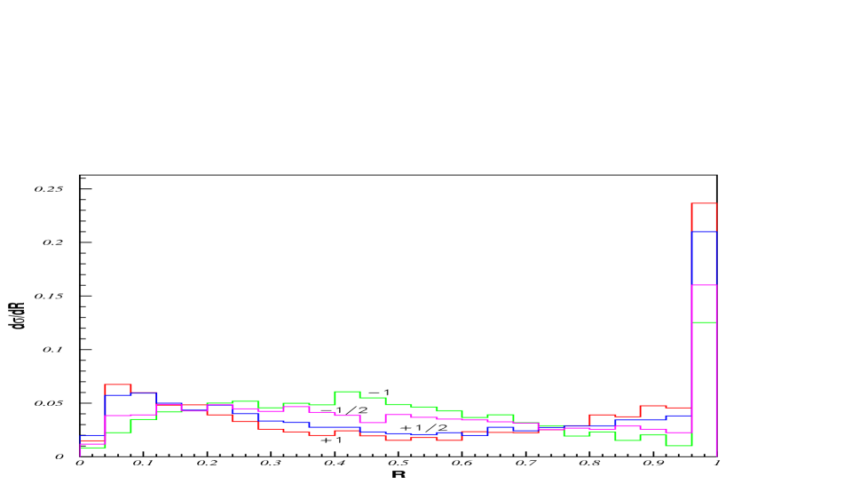
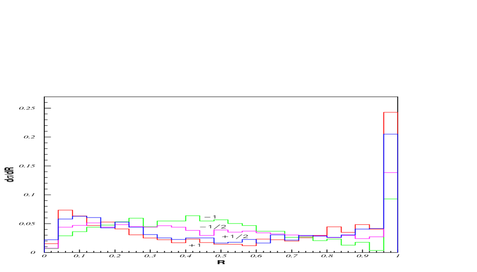
Figure 1: The normalized distributions in the fraction of $\tau$-jet momentum carried by the charged track for $P_{\tau}$= +1, +1/2, -1/2 and -1. The upper and lower panels correspond to $p^{T}_{\tau-jet}>$25 GeV and $p^{T}_{\tau-jet}>$50 GeV respectively.

Fig.1 shows the resulting R distributions for the four $P_{\tau}$ values corresponding to $p^{T}_{\tau-jet}>25$ GeV(upper pannel) and $p^{T}_{\tau-jet}>50$ GeV(lower panel). The last bin near $R=1$ represents the $\tau^{\pm}\rightarrow\pi^{\pm}\nu$ contribution. Thus the R distribution is expected to peak at the two ends for $P_{\tau}>$0 states while it is expected to peak near the middle along with a depleted $\tau^{\pm}\rightarrow\pi^{\pm}\nu$ contribution for $P_{\tau}<$0. The difference increases with increasing $p^{T}_{\tau-jet}$ cut as expected from eq. 11-14. But even for the $p^{T}_{\tau-jet}>$25 GeV cut of eq. 15, the differences in the R distribution are sufficient to distinguish the four models from one another.

Fig.2 shows the fraction of events in the interval 0.2$<R<$0.8,

$$f=\frac{\sigma(0.2<R<0.8)}{\sigma_{tot}}$$ (22)

against the $\tau$ polarization. This fraction is seen to decrease from 65% at $P_{\tau}=-$1 to 35% at $P_{\tau}=$+1 for the $p^{T}_{\tau-jet}>$25 GeV cut (solid lines); and the decrease becomes steeper for the harder $p^{T}_{\tau-jet}>50$ GeV cut (dashed lines) as expected. Thus this fractional cross section can be used to measure $P_{\tau}$. In case the R $<0.2$ region is inaccessible due to the difficulty in $\tau$ identification for a soft charged track, the cross section $\sigma(0.2<R)$ can be used for normalization in the denominator of eq. 22. To get a rough estimate of the size of uncertainty in the measurement of $P_{\tau}$, we have shown the predictions using the ALEPH and CLEO parameterizations of $\tau$ decay [13] by two lines for each case. The horizontal spread between them corresponds to a $\Delta P_{\tau}=\pm 0.03$ ($\pm$0.05) near $P_{\tau}$=$-$1($+$1). One should of course add to this the uncertainty in the measurement of f (eq. 22). However being a ratio of measured cross-sections this quantity is dominated by the statistical error, which is $\sim$0.01 corresponding to $\sim 10^{4}$ signal events. Hence the dominant error in $P_{\tau}$ measurement is expected to come from the parametrization of $\tau$ decay, as represented by the horizontal spread between the two lines of fig.2. It should be noted here that even a conservative estimate of $\Delta P_{\tau}=\pm$0.1 would imply that the above four models can be distinguished from one another at the 5$\sigma$ level.

B) Partial Determination of SUSY Parameters:

In this section we shall assume the mass relation of eq.2 between the two electroweak gauginos, which holds in a fairly broad class of SUSY models. It holds in most SUSY models satisfying GUT symmetry, in which case the gaugino masses arise from the vev of a GUT singlet chiral superfield. This includes the SUGRA models with nonuniversal scalar masses. It holds for the GMSB as well. We shall assume that the $\tan\beta$ parameter can be independently measured from the Higgs sector at LHC or ILC. Moreover we shall assume that the absolute scale of one of the SUSY masses, representing some combination of $M_{1}$, $M_{2}$ and $\mu$ can also be measured independently. Then the relative magnitude of the $M_{1}$ and the $\mu$ parameters can be estimated from the $\tau$ Polarization.

We have calculated the composition of $\tilde{Z}_{1}$, as a function of the ratio $M_{1}/|\mu|$, assuming the $\tilde{Z}_{1}$ mass of as in eq.16 to fix the SUSY mass scale. Fig. 3 shows the resulting $P_{\tau}$ from eqs.(9,10) for two representative values of $\tan\beta=40$ and 10 and $\cos\theta_{\tilde{\tau}}=$ 0.5 and 0.2. It shows that $P_{\tau}$ is insensitive to this ratio for $M_{1}/|\mu|<$0.5 at $\tan\beta$=40 (b,d) and $M_{1}/|\mu|<$1 at $\tan\beta$=10(a,c). But above these limits one can measure this ratio to an accuracy of $\sim$ 10% with a $\Delta P_{\tau}=$0.1.

C) Complete determination of $EW$ SUSY parameters in association with chargino $(\tilde{W}_{1})$ mass and cross section measurements:

In most of the SUSY benchmark points of Ref. [5] discussed above, the lighter chargino $\tilde{W}_{1}$ mass lies in the range of 200-250 GeV. Therefore one hopes to see pair production of chargino in the first phase of ILC with a CM energy of $\sim$500 GeV. In that case one can estimate some of the above mentioned SUSY parameters from this process, as discussed in  [17]. In particular the mass and the composition of $\tilde{W}_{1}$ can be easily obtained in terms of $M_{2},\mu$ and $\tan\beta$ by diagonalizing the chargino mass matrix,

$${\cal M}_{\tilde{c}}=\left(\begin{array}[]{cc}M_{2}&{\sqrt{2}}M_{W}\sin\beta\\ {\sqrt{2}}M_{W}\cos\beta&\mu\end{array}\right)\qquad$$ (25)

Thus one knows the coupling of a $\tilde{W}_{1}$ pair to the Z boson in terms of these three parameters, while it has the universal EM coupling to $\gamma$. With a right polarized electron beam the $\tilde{W}_{1}$ pair production proceeds only through s-channel $\gamma$ and $Z$ exchanges. Thus by measuring this production cross section $\sigma_{R}$ along with the $\tilde{W}_{1}$ mass from a threshold scan, one can estimate the composition of $\tilde{W}_{1}$. These two measurements determine two of the above three parameters. Hopefully the third parameter ($\tan\beta$) can be independently estimated from the Higgs sector at the LHC or the ILC, as mentioned above. Alternatively, one can measure the $\tilde{W}_{1}$ pair production cross sections with left and transversally polarized electron beams, $\sigma_{L}$ and $\sigma_{T}$. These two cross sections get contributions from t-channel $\tilde{\nu}_{e}$ exchange along with the s-channel $\gamma$ and $Z$ exchanges. Thus they depend on $\tilde{\nu}_{e}$ mass along with the above three parameters. Nonetheless one can combine the three cross sections $\sigma_{L},\sigma_{R}$ and $\sigma_{T}$ along with the $\tilde{W}_{1}$ mass measurement to determine all the four parameters, as discussed in  [17]. That would leave one SUSY parameter from the EW sector, $(M_{1})$, which cannot be directly measured at ILC in the absence of a $\tilde{Z}_{1}$ pair production signal. However one can use instead the $P_{\tau}$ from the $\tilde{\tau}_{1}\to\tau\tilde{Z}_{1}$ decay to determine this parameter. Recall that along with $M_{1}$ $P_{\tau}$ has a dependence also on the stau sector mixing angle and $\tan\beta$. As a matter of fact, the role of $P_{\tau}$ to probe the Higgsino component in the $\tilde{Z}_{1}$, especially at large $\tan\beta$, has been emphasized[8]. As mentioned above, in the discussion we are assuming that these two parameters may be determined from other sectors. Of course, in a global fit, $P_{\tau}$ will be one of the important variables in a model independent determination of $\theta_{\tau},M_{2},M_{1},\mu$ and $\tan\beta$.

Since both $M_{2}$ and $|\mu|$ would be known from chargino production, the $\tau$ polarization can be used to determine $M_{1}$ relative to either one of them. For illustrative purpose we have assumed $M_{2}=250$ GeV and three values of the ratio $|\mu|/M_{2}=$2, 1 and 0.5. As in case of Fig.3 in this illustration also, we take two widely different sets of $\tan\beta,\cos\theta_{\tau}$, chosen to span the range of expectations for these two, to demonstrate the dependence of $P_{\tau}$ on them. The resulting polarization($P_{\tau}$) is shown against $M_{1}/M_{2}$ in Fig.4 for $\tan\beta=40$, $\cos\theta_{\tau}$=0.5 and in Fig.5 for $\tan\beta$=10, $\cos\theta_{\tau}$=0.2. One sees from these figures that while $P_{\tau}$ is flat for extreme values of $M_{1}/M_{2}$, it is a sensitive function of this ratio for $0.5\buildrel\scriptscriptstyle<\over{\scriptscriptstyle\sim}M_{1}/M_{2}\buildrel\scriptscriptstyle<\over{\scriptscriptstyle\sim}2$. One can measure the ratio $M_{1}/M_{2}$ to an accuracy of 5-10% over this interval with a $\Delta P_{\tau}=$0.1. Thus knowing both $\mu$ and $M_{2}$ from $\tilde{W}_{1}$ production one can use $P_{\tau}$ to determine $M_{1}$ relative to $M_{2}$. In other words one can combine the $\tilde{W}_{1}$ mass and cross section measurements with the $\tau$ polarization to make a complete determination of the EW SUSY parameters.

It should be mentioned here that there is an alternative method of determining $M_{1}$ from kinematic distributions as suggested in ref. [18]. We are not in a position to make a comparative assessment of the relative merits of the two methods. Instead we would like to emphasize their complementarity. The kinematic distributions probe the LSP($\tilde{Z}_{1}$) mass, while the $P_{\tau}$ measurement probes its composition. In this respect $P_{\tau}$ plays a role analogous to the production cross section of chargino ($\tilde{W}_{1}$). Note that one can combine the measurements of $\tilde{W}_{1}$ mass and composition via threshold scan and the production cross section $\sigma_{R}$ with those of $\tilde{Z}_{1}$ mass and composition via the kinematic distribution method and $P_{\tau}$. Thereby one can determine all the four parameters ($\mu,M_{1},M_{2}$ and $\tan\beta$) with only the right polarized electron beam. On the other hand one can combine these four measurements with $\sigma_{L}$ and $\sigma_{T}$. Then the resulting redundancy of information can be used as a consistency check of the CP conserving MSSM. Alternatively, it can be used to extend the analysis and probe for CP violation in MSSM [19].

Figure 2: The fractional cross sections in the interval $0.2<R<0.8$ (eq. 22) plotted against $\tau$ polarization for $p^{T}_{\tau-jet}>$25 GeV (solid lines) and $p^{T}_{\tau-jet}>$50 GeV (dashed lines). The upper and lower lines for each case correspond to the parameterizations of $\tau$ decay by the ALEPH and the CLEO collaborations [13] respectively.

Figure 3: Polarization of $\tau$ shown against $M_{1}/|\mu|$ for a fixed value of $m_{\tilde{Z}_{1}}=100$ GeV and $M_{1}/M_{2}$=0.5 and different sets of parameters:(a)$\tan\beta=10,cos\theta_{\tau}=$0.5; (b)$\tan\beta=40,cos\theta_{\tilde{\tau}}=$0.5; (c)$\tan\beta=10,cos\theta_{\tilde{\tau}}=$0.2; (d)$\tan\beta=40,cos\theta_{\tilde{\tau}}=$0.2.

Figure 4: Polarization of $\tau$ shown against $M_{1}/M_{2}$ for a fixed value of $\tan\beta=40,cos\theta_{\tau}=$0.5, $M_{2}=$250 GeV and $|\mu|/M_{2}=$0.5,1,2.

Figure 5: Same as in Fig.4, but for $\tan\beta=10,cos\theta_{\tau}=$0.2.

References

- [1] See e.g, Physics interplay of the LHC and the ILC: LHC/LC study group, hep-ph/0410364 and references to earlier LC physics reports therein.
- [2] For reviews see, e.g Perspectives in Supersymmetry, ed. G. L. Kane, World Scientific(1998). Theory and Phenomenology of sparticles: M. Drees, R.M. Godbole and P. Roy, World Scientific, Jan. 2004.
- [3] Review of Particle Physics: S. Eidelman et al, Phys. Lett. B592(2004) 1.
- [4] The Higgs WG summary report in the workshop on Physics at TeV colliders, Les Houches, 2001 [ D. Cavalli et al, hep-ph/0203056].
- [5] Compilation of SUSY particle spectra from Snowmass 2001 benchmark models: B. C. Allanach et al , Euro Phys. J. C25(2002)113; N. Ghodbane and H. U. Martyn, hep-ph/0201233.
- [6] J. R. Ellis et al, Phys. Lett. B155(1985)381; M. Drees, Phys. Lett. B158(1985)409; G. Anderson,et al, Phys. Rev. D61(2000)095005; K. Huitu et al, Phys. Rev. D61(2000)035001; U. Chattopadhyay and P. Nath, Phys. Rev. D65(2002)075009. U. Chattopadhyay and D. P. Roy, Phys. Rev. D68(2003)033010.
- [7] M. M. Nojiri, Phys. Rev. D51(1995)6281; M.M. Nojiri, K.Fujii and T. Tsukamoto, Phys. Rev. D54(1996)6756.
- [8] E. Boos, H.U. Martyn, G. Moortgat-Pick, M. Sachwitz, A. Sherstnev and P. M. Zerwas, Euro. Phys.J. C30(2003)395.
- [9] B. K. Bullock, K. Hagiwara and A. D. Martin, Phys. Rev. Lett. 67(1991)3055, Nucl. Phys. B395(1993)499.
- [10] S. Raychaudhuri and D. P. Roy, Phys. Rev. D52(1995)1556; D53(1996)4902; D. P. Roy, Phys. Lett. B459(1999)607.
- [11] K. A. Assamagan, Y. Coudou and A. Deandrea, Eur. Phys. J C4(2002)9; D. Denegri et al CMS note 2001/032, hep-ph/0112045.
- [12] M. Guchait and D. P. Roy, Phys. Lett. B535(2002)243; B541(2002)356.
- [13] S. Jadach, Z. Was,R. Decker and J. H. Kuehn, Comput.Phys.Commun.76(1993)361; P. Golonka et al, hep-ph/0312240 and references therein.
- [14] T. Sjostrand, P. Eden, C. Friberg, L. Lonnblad, G. Miu, S. Mrenna and E. Norrbin, Computer Physics Commun. 135(2001)238.
- [15] L. Randall and R. Sundrum, Nucl. Phys. B557(1999)79; G. F. Giudice, M. A. Luty, H. Murayama and R. Rattazi, JHEP, 9812(1998)027.
- [16] D. A. Dicus, B. Dutta and S. Nandi, Phys. Rev. D56(1997)5748; B. Dutta, D. J. Miller and S. Nandi, Nucl. Phys. B544(1999)451; H. Baer et al Phys. Rev D60(1999)055001, D62(2000)095007.
- [17] S. Y. Choi, M. Guchait, J. Kalinowski and P. M. Zerwas, Phys. Lett B479(2000)235; S. Y. Choi, A. Djouadi, M. Guchait,J. Kalinowski, H.S.Song and P.M.Zerwas, Eur. Phys. J. C14(2000)535.
- [18] S. Y. Choi, J. Kalinowski, G. Moortgat-Pick, P. M. Zerwas, Euro. Phys. J. C22(2001)563.
- [19] T. Gajdosik, R. M. Godbole and S. Kraml, JHEP, 409(2004)51.