DESY 04-224 ISSN 0418-9833
hep-ph/0411300
November 2004
Inclusive Production of Single Hadrons with Finite Transverse Momenta
in Deep-Inelastic Scattering at Next-to-Leading Order
Abstract
We calculate the cross section for the inclusive production of single hadrons with finite transverse momenta in deep-inelastic scattering at next-to-leading order (NLO), i.e. through , in the parton model of QCD endowed with non-perturbative parton distribution functions (PDFs) and fragmentation functions (FFs). The NLO correction is found to produce a sizeable enhancement in cross section, of up to one order of magnitude, bringing the theoretical prediction to good agreement with recent measurements for neutral pions and charged hadrons at DESY HERA. This provides a useful test for the universality and the scaling violations of the FFs predicted by the factorization theorem. Such comparisons can also be used to constrain the gluon PDF of the proton.
PACS numbers: 12.38.Bx, 12.39.St, 13.87.Fh, 14.40.Aq
1 Introduction
The predictive power of the parton model of quantum chromodynamics (QCD) lies in the factorization theorem. In deep-inelastic scattering (DIS), factorization in short- and long-distance parts allows us to describe the observed cross sections of inclusive hadron production as a convolution of the partonic cross sections with non-perturbative parton density functions (PDFs) and fragmentation functions (FFs) [1]. Single-hadron inclusive production in electron-proton DIS,
| (1) |
occurs partonically already in the absence of strong interactions, at , where is the strong-coupling constant, when one parton of the proton (a quark) interacts with the lepton current and fragments into the hadron (naïve parton model). If the virtuality of the four-momentum transfer satisfies , where denotes the -boson mass, then process (1) is essentially mediated by a virtual photon (), while the contribution from -boson exchange is negligible. In the following, this is the situation we are interested in.
Since we are interested in perturbative QCD effects, we require the hadron to carry non-vanishing transverse momentum () in the centre-of-mass (c.m.) frame of the virtual photon and the incoming proton. At leading order (LO), the corresponding partonic subprocesses thus contain two partons in the final state, one of which fragments into the hadron, while the other one balances the transverse momentum. At next-to-leading order (NLO), three-parton final states contribute to the real correction, while the virtual correction arises from one-loop diagrams with two final-state partons.
The investigation of single-hadron production is interesting for several reasons. First of all, it provides a test of perturbative QCD and of factorization. Apart from the partonic cross sections obtainable from perturbative QCD, the theoretical predictions essentially depend on universal PDFs and FFs. In particular, the FFs, which are fitted to electron-positron-annihilation data, may be tested with regard to their universality. Furthermore, the theoretical predictions allow for a direct comparison with experimental data, without resorting to any kind of Monte Carlo model to simulate the hadronization of the outgoing partons. Thus, we may expect very meaningful results. Moreover, the theoretical predictions are directly sensitive to the gluon PDF of the proton with the potential to constrain the latter.
On the experimental side, precise data were collected by the H1 [2, 3, 4] and ZEUS [5, 6] Collaborations at the collider HERA at DESY. They refer to mesons in the forward region [3, 4], with small angles with respect to the proton remnant, and to charged hadrons [2, 5, 6].
More than 25 years ago, the cross section of process (1) with finite transverse momentum of the hadron was calculated by Méndez [7] at LO, to . Since QCD corrections are typically large and we are confronted with precise experimental data, it is desirable to compare these data with predictions of at least NLO accuracy, including the terms of . For this purpose, a first NLO QCD prediction was computed in Ref. [8], neglecting the longitudinal degrees of freedom of the virtual photon.
The theoretical description can be rendered more reliable by resumming the leading logarithmic contributions of the perturbation expansion. In this sense, the Balitsky-Fadin-Kuraev-Lipatov (BFKL) [9] and Dokshitser-Gribov-Lipatov-Altarelli-Parisi (DGLAP) [10] equations resum at LO the and contributions, respectively, where is the Bjorken variable and is the cut-off scale for the perturbative evolution. Disregarding the fact that these resummations are just approximations, they evidently fail in the kinematic regions of large values and small values, respectively.
In this paper, we perform a full NLO QCD calculation, also taking into account the longitudinal degrees of freedom of the virtual photon. We encounter ultraviolet (UV) and infrared (IR) singularities, which we all regularize using dimensional regularization. In order to overcome the difficulties in connection with the IR singularities emerging in different parts of the NLO correction, we employ the dipole subtraction formalism [11]. In contrast to the more conventional phase-space slicing method, there is no need to introduce any unphysical parameter to cut the phase space into soft, collinear, and hard regions. Moreover, all cancellations of IR singularities occur before any numerical phase-space integration is performed. We thus conveniently obtain numerically stable predictions.
An independent calculation was recently presented in Ref. [12], where the matrix elements of the hard-scattering processes were adopted from the DISENT program package [13]. In Ref. [12], the phase-space slicing method was applied to handle the IR singularities. Another related work, focusing on fracture functions of the proton, was published in two parts, related to incoming gluons [14] and quarks [15].
2 Analytical analysis
According to the factorization theorem [1], the differential cross section for process (1) is given as a convolution of the hard-scattering cross sections with the PDFs of the proton and FFs of hadron , as
| (2) |
where and are the factorization scales related to the initial and final states and the sum runs over all tagged initial- and final-state partons, and , respectively. As usual, the dimensionless variables , , and are defined as , , and with respect to the partonic four-momenta and , and their barred counterparts , , and with respect to the hadronic four-momenta. We have , where is the square of the c.m. energy. It is convenient to describe the kinematics in the c.m. frame of the virtual photon and the incoming parton as is done in Fig. 1, where we take the three-momentum of the virtual photon to point along the axis and the three-momenta of the incoming and scattered electrons to lie in the - plane. Then, the azimuthal angle of the hadron is enclosed between the plane spanned by the three-momenta of the incoming and scattered electrons and the one spanned by those of the virtual photon and the outgoing parton .

The hard-scattering cross sections may be written as contractions of a lepton tensor with hadron tensors , as
| (3) |
where is Sommerfeld’s fine-structure constant. If the virtual photon and the initial-state parton are both unpolarized, then there cannot be any dependence on the azimuthal angle . Integrating over the latter, we find the decomposition
| (4) |
where , , and .
The partonic subprocesses contributing at LO are
| (5) | |||||
| (6) | |||||
| (7) |
where it is understood that the first of the final-state partons is the one that fragments into the hadron . Here, , where is the number of active quark flavours, which are ordered according to their masses, i.e., , , , , and , and we identify . There are two Feynman diagrams for each of the processes (5)–(7). The matrix elements of processes (5)–(7) are interrelated through crossing symmetry. Owing to charge-conjugation () invariance, the counterparts of processes (5)–(7) with quarks and antiquarks interchanged yield equal cross sections and do not have to be calculated separately. However, this is not generally true for the PDFs and FFs. Therefore, we have to explicitly sum over all possible pairings of partons and in Eq. (2). For the reader’s convenience, the LO expressions for the Lorentz invariants and in Eq. (4) are listed in Appendix A. They are of and proportional to , where denotes the electric charge of quark in units of the positron charge.
In order to determine the NLO correction to the cross section of processes (1), we have to compute the virtual and real corrections of to the hadron tensors. We then encounter a rather involved pattern of singularities. All these singularities are regularized using dimensional regularization with space-time dimensions yielding poles in in the physical limit . The integrations over the loop four-momenta in the virtual correction lead to UV and IR singularities, where the IR ones comprise both soft and collinear singularities. All UV singularities are removed through the renormalizations of the wave functions and the strong-coupling constant. The remaining soft and collinear singularities cancel partly against counterparts originating from the phase-space integration of the real correction. The remaining collinear poles have to be factorized into the bare PDFs and FFs so as to render them finite.
The virtual correction is obtained as the interference of the Born and one-loop matrix elements. The latter receive contributions from self-energy, triangle, and box diagrams. These involve two-, three-, and four-point tensor integrals, which are reduced to scalar integrals via tensor reduction [16]. The scalar integrals contain both UV and IR singularities. They are computed analytically in dimensional regularization. Our analytic expressions for the contractions of the resulting hadron tensors with agree with the literature [17]. The virtual correction is renormalized in the modified minimal-subtraction () scheme and thus UV finite.
The partonic subprocesses contributing to the real correction read
| (8) | |||||
| (9) | |||||
| (10) | |||||
| (11) | |||||
| (12) | |||||
| (13) | |||||
| (14) | |||||
| (15) |
where with . As in processes (5)–(7), the first partons in the final states of processes (8)–(15) are taken to fragment into the hadron . The order in which the residual final-state partons appear is irrelevant. There are eight Feynman diagrams for each of the processes (8)–(13) and four ones for each of the processes (14) and (15). Crossing symmetry interrelates the matrix elements of processes (8)–(11), those of processes (12)–(13), and those of processes (14)–(15). The cross sections of processes (8)–(15) are of . Those of processes (8)–(13) are proportional to , while, at first sight, those of processes (14)–(15) contain pieces proportional to , , and . However, in the case of process (14), the piece proportional to vanishes by Furry’s theorem, as is explained below. The squared matrix elements of processes (8)–(11) involve one quark trace, those of processes (12) and (13) contain pieces with one or two quark traces, and those of processes (14) and (15) involve two quark traces. Due to invariance, the counterparts of processes (8)–(15) with quarks and antiquarks interchanged yield equal cross sections. Notice that, in the case of process (15), we have to distinguish between the case where the tagged quarks and are both particles or anti-particles and the case where one is a particle and the other one is an anti-particle. Processes (8) and (13) each contain two identical untagged partons in the final state, so that their cross sections receive a statistical factor of 1/2 to avoid double counting in the phase space integration. We derived the matrix elements of processes (8)–(15) in two steps. First, we calculated the ones of the corresponding processes of annihilation via a virtual photon, which may also be found in Ref. [18]. Then, we employed crossing symmetry. The squared matrix elements of processes (8)–(15), excluding the Furry terms discussed below, are also implemented in the DISENT program package [13]. Performing a numerical comparison with the latter, we find agreement.
In Ref. [18], the squared matrix elements, which may be visualized as cut diagrams, are classified with respect to colour factors. One specific class, called F terms, contains all cut diagrams with two fermion loops, which are both coupled to three vector bosons, namely to one photon and two gluons. This class constitutes a gauge-parameter-independent subset of the NLO correction. The cut diagram of one specific member of this class is shown in Fig. 2, where the on-shell quarks are indicated by numbers. As was noticed in Ref. [18], by Furry’s theorem, each cut diagram within this class exactly cancels against one counterpart in which one fermion-number flow is reversed if the on-shell quarks associated with the loop whose fermion-number flow is reversed are not tagged in the experiment, i.e. if the three-momenta of these quarks are integrated over. This argument is also true in the case where only one fermion charge is identified, for instance in single-hadron production by annihilation, since there is still a counterpart diagram where the other fermion-number flow is reversed. In our case, there are two tagged partons, one coming from the proton and one fragmenting into the hadron . Suppose the two tagged partons are the quarks 1 and 2 in the cut diagram of Fig. 2. This situation can occur for processes (12) and (13), which involve only one quark flavour, and for process (15), which involves two different quark flavours. Then, the Furry cancellation is impeded because there is no counterpart diagram. Thus, we are not allowed to omit this class of cut diagrams in our calculation. The corresponding squared matrix elements are listed in Appendix B.

The differential cross sections of processes (8)–(15) have to be integrated over the three-momenta of the second and third final-state partons keeping the three-momentum of the first one fixed. Performing the phase-space integrations, we encounter IR singularities of the soft and/or collinear types, which, for consistency with the virtual correction, must be extracted using dimensional regularization. It is convenient to do this by means of the dipole subtraction formalism [11]. The general idea of this formalism is to subtract from the contribution to the real correction due to a given partonic subprocess some artificial counterterm which has the same point-wise IR-singular behaviour in space-time dimensions as the considered part of the real correction itself. Thus, the limit can be performed, and the phase space integration can be evaluated numerically in four dimensions. The artificial counterterm is constructed in such a way that it can be integrated over the one-parton subspace analytically leading to poles in . Adding the terms thus constructed to the virtual correction, the IR singularities of the latter are cancelled analytically. In the present case, where the three-momenta of two tagged partons need to be kept fixed, additional, more complicated artificial counterterms appear than in situations where only one parton is tagged, such as inclusive jet production. A technical advantage of the dipole subtraction method compared to the phase space slicing method is that all IR singularities cancel before any numerical integration is performed. Furthermore, there is no need to introduce a slicing parameter to separate soft and/or collinear phase space regions from the remaining hard region, which needs to be tuned in order to obtain a numerically stable result. For the factorization of the collinear singularities associated with the tagged partons, we choose the scheme. In turn, we have to employ PDFs and FFs which are defined in the same scheme.
Finally, we end up with two contributions, the real correction with the artificial counterterms subtracted and the virtual correction with the integrated artificial counterterms included, which are both finite in the physical limit and can be integrated over their three- and two-particle phase spaces, respectively, in three spacial dimensions. These integrations are performed numerically using a custom-made C++ routine. On the other hand, all algebraic calculations are executed with help of the symbolic-manipulation package FORM [19].
3 Numerical results
We are now in a position to present our numerical results for the cross section of single-hadron inclusive production in DIS. We start by specifying our input. We work in the renormalization and factorization scheme with massless quark flavours. At NLO (LO), we employ set CTEQ6M (CTEQ6L1) of proton PDFs by the Coordinated Theoretical-Experimental Project on QCD (CTEQ) [20], the NLO (LO) set of FFs for light charged hadrons (, , and ) by Kniehl, Kramer, and Pötter (KKP) [21], and the two-loop (one-loop) formula for with asymptotic scale parameter MeV (165 MeV) [20]. This value is compatible with the result MeV ( MeV) determined in Ref. [22]. We approximate the FFs as
| (16) |
where refers to the sum of the and mesons, which is supported by LEP1 data of hadronic -boson decays [23]. Furthermore, we assume the charged hadrons to be exhausted by the charged pions, charged kaons, protons, and antiprotons, viz
| (17) |
For simplicity, we identify the renormalization scale and the initial- and final-state factorization scales, and , respectively, and relate them to the characteristic dimensionful variables and by setting , where is a dimensionless parameter of order unity introduced to estimate the theoretical uncertainty due to unphysical-scale variations. As usual, we consider variations of between 1/2 and 2 about the default value 1.
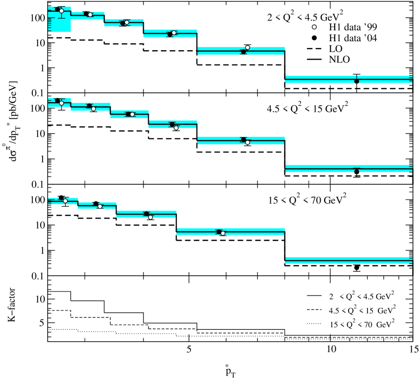
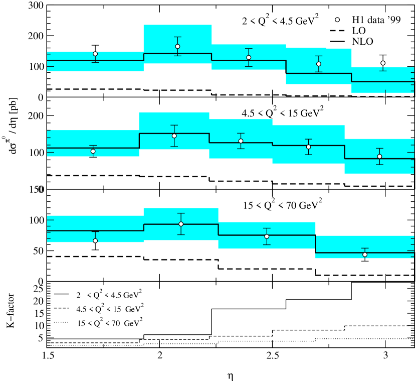
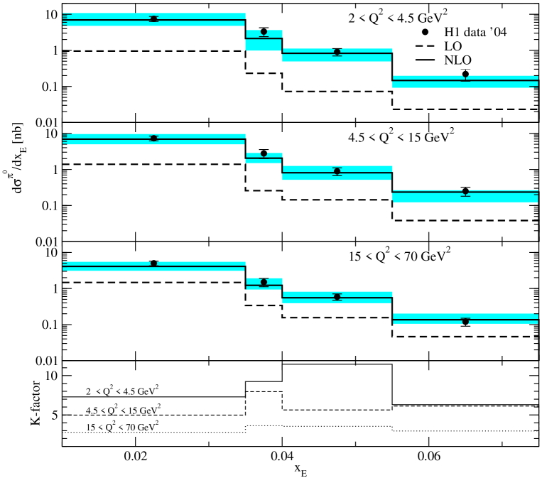
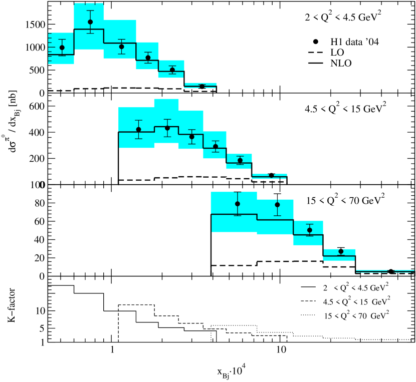
We now compare our theoretical predictions with HERA data on mesons in the forward region from the H1 Collaboration [3, 4] and on charged hadrons in the current-jet region from the ZEUS Collaboration [5]. We start by discussing the H1 data [3, 4], which were taken in DIS of positrons with energy GeV on protons with energy GeV in the laboratory frame, so that GeV, during the running periods 1996 and 1996/1997, and correspond to integrated luminosities of 5.8 and 21.2 pb-1, respectively. In Refs. [3, 4], the mesons were described by their transverse momentum in the c.m. frame and by their angle with respect to the proton flight direction, their pseudorapidity , and their energy in the laboratory frame. They were detected within the acceptance cuts GeV or 3.5 GeV, , and . The DIS phase space was restricted to the kinematic regime defined by and GeV2. The cross section was measured differentially in [3, 4], [3], [4], and [3, 4] for various intervals, differentially in for various intervals [4], and differentially in [3]. The differential cross sections , , , , and presented in Refs. [3] (open circles) and [4] (solid circles) are compared with our LO (dashed histograms) and NLO (solid histograms) predictions in Figs. 3–7, respectively. In Figs. 3, 4, 5(a), and 6(a), the upper three frames refer to the intervals GeV2, GeV2, and GeV2. In Fig. 5(b), the upper three frames refer to the intervals , , and . In Fig. 6(b), the upper three frames refer to the intervals GeV2, GeV2, and GeV2. In all figures, the minimum- cut is GeV, expect for Fig. 6(b), where it is GeV. In Figs. 3–7, the shaded bands indicate the theoretical uncertainties of the NLO predictions due to the variation described above. The factors, defined as the NLO to LO ratios of our default predictions, are shown in the downmost frames of Figs. 3–7.
![[Uncaptioned image]](/html/hep-ph/0411300/assets/x6.png)
![[Uncaptioned image]](/html/hep-ph/0411300/assets/x8.png)
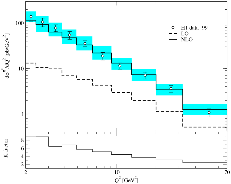
We observe from Figs. 3–7, that the H1 data generally agree with our NLO predictions within errors, while they significantly overshoot our default LO predictions. Indeed, the factors always exceed unity and even reach one order of magnitude at low values of , , or . Not only do the LO predictions disagree with the H1 data in their normalizations, but they also exhibit deviating shapes. On the other hand, under the effect of asymptotic freedom, the factors approach unity for increasing values of , i.e. for increasing values of and/or .
There is an obvious explanation for the sizeable factors at low values of in terms of the different kinematic constraints at LO and NLO. The LO processes (5)–(7) are , and their cross sections are sensitive to collinear singularities only as . By contrast, processes (8)–(15) contributing to the real NLO correction are , so that collinear configurations can also arise for finite values of . After mass factorization of the corresponding collinear singularities, the finite remainders can be sizeable, leading to large NLO corrections. A similar line of reasoning was presented in Ref. [12].
Unfortunately, the theoretical uncertainties in our NLO predictions due to variation are rather sizeable, especially at low values of , , or , where the factors themselves are abnormally large. This is partly related to the opening of new partonic production channels at NLO, which are still absent at LO, namely those of Eqs. (11), (13), and (15). Obviously, a reduction in dependence can only be expected to happen at next-to-next-to-leading order (NNLO), which is beyond the scope of this work.
Besides the freedom in the choice of the renormalization and factorization scales, there are other sources of theoretical uncertainty, including the variations of the PDF and FF sets. However, in view of the considerable spread in cross section induced by the moderate variations described above, we conclude that the residual sources of theoretical uncertainty are of minor importance. Furthermore, we must bear in mind that the factorization theorem itself is only valid up to terms of , which may become large in the low- range.
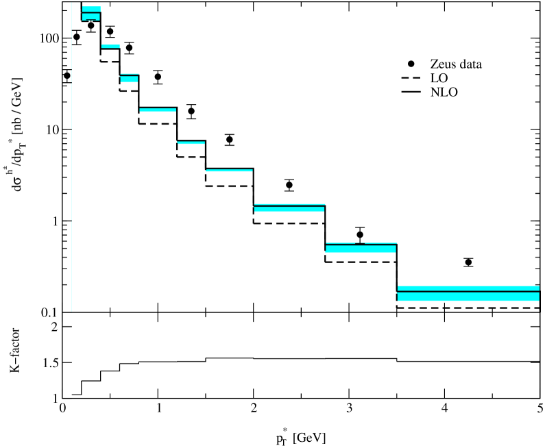
We now turn to the ZEUS data on charged hadrons [5], which were produced in DIS of electrons with energy GeV on protons with energy GeV in the laboratory frame, giving GeV, during the 1993 running period and correspond to an integrated luminosity of 0.55 pb-1. They refer to the DIS phase space defined by GeV2 and GeV, where is the invariant mass, with , and come as multiplicities differential in or Feynman’s variable , where is the projection of the hadron three-momentum onto the flight direction of the virtual photon in the c.m. frame, and normalized to the total number of DIS events. Unfortunately, the distribution of the multiplicity includes charged hadrons with values down to zero, while our NLO analysis is only valid for finite values of , so that a comparison is impossible. However, a comparison is feasible for the distribution [5], which includes charged hadrons with . The differential cross section may be obtained using the conversion formula [24]
| (18) |
where is the total cross section in the DIS regime specified above,
| (19) |
At LO, we have [25]
| (20) |
where and . Using the parameterization [24]
| (21) |
where GeV2, , , and , obtained from a fit to ZEUS data, we thus find nb assuming the errors on , , and to be statistically independent. This nicely agrees with the result nb obtained in the parton model of QCD, where [25]
| (22) |
using set CTEQ6L1 [20] of proton PDFs with . For consistency, we use the ZEUS result for to convert the ZEUS data for [5]. The result for thus obtained (solid circles) is compared with our LO (dashed histogram) and NLO (solid histogram) predictions in Fig. 8 (upper frame). As in Figs. 3–7, the shaded band indicates the theoretical uncertainty in the NLO prediction due to the variation described above, and the factor is also shown (lower frame). Again, our NLO prediction leads to a better description of data than our LO one. Here, the factor takes more moderate values than under H1 kinematic conditions, being of order 1.5 or below. As explained above, our LO and NLO predictions break down in the limit . This drawback can be fixed by the resummation of multiple parton radiation, as demonstrated in Ref. [26] on the basis of the LO result.
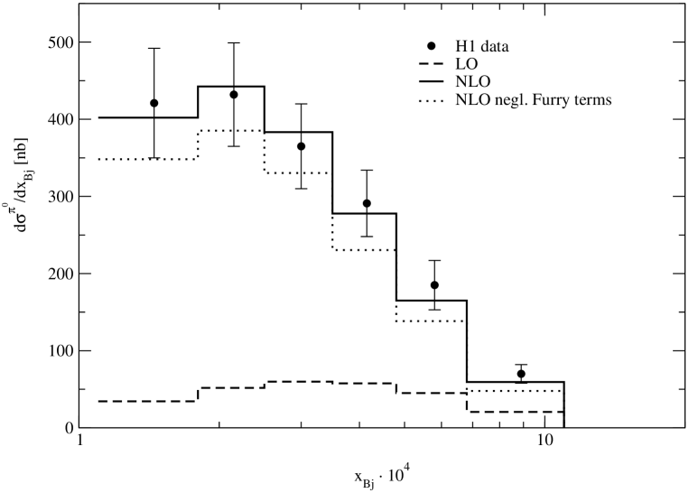
In Section 2, we explained why the Furry terms do not vanish in our case, in contrast to inclusive jet production in DIS [13]. It is interesting to investigate their importance quantitatively. To this end, we reconsider the differential cross sections for , GeV2, GeV, , and and for GeV2, GeV, and , which we already studied in the second frame of Fig. 6(a) and the first frame of Fig. 8, respectively, and turn off the Furry terms in our default NLO prediction. The results are shown together with our default LO and NLO predictions and the H1 [4] and ZEUS [5] data in Figs. 9(a) and (b), respectively. We observe that the Furry terms are very important. In Fig. 9(a), they account for roughly 20% of the NLO correction, while, in Fig. 9(b), they practically exhaust the latter.
![[Uncaptioned image]](/html/hep-ph/0411300/assets/x12.png)
Figure 9: Continued.
We expect our fixed-order predictions to break down in three extreme kinematic regimes corresponding to the limits (i) ; (ii) or, equivalently, or ; and (iii) . Case (i) corresponds to the photoproduction limit, in which the resolved-photon contribution gains importance, especially at small values of and/or . Case (ii) is related to the possibility that the observed hadron originates from the proton remnant, so that the notion of fracture functions is invoked. Case (iii) is expected to correspond to the realm of BFKL [9] dynamics, although it is unclear precisely where the onset of the latter is supposed to be located. Our analysis is puristic in the sense that resolved virtual photons, fracture functions, and BFKL dynamics are disregarded, so as to test their actual relevance in the confrontation of the QCD-improved parton model with the experimental situation of Refs. [3, 4, 5]. Let us now scrutinize these issues. Doing this, however, we have to bear in mind that the theoretical uncertainty in our NLO predictions due to the arbitrariness in the choice of the unphysical scales is particularly large in these corners of phase space, so that any conclusions are likely to be premature prior to the advent of a full NNLO analysis. From Fig. 7, we observe that our NLO prediction for tends to undershoot the H1 data [3] in the low- range, so that there is indeed some room for a resolved-photon contribution. Similar conclusions were reached in Ref. [27]. On the other hand, we see from Fig. 4 that the H1 data for [3] significantly exceed our NLO prediction in the very forward region, i.e. in the rightmost bin, for low values of . In fact, for GeV2, the measured distribution exhibits a plateau in the upper range, whereas the NLO prediction is rapidly suppressed by the shrinkage of the available phase space for increasing value of . This plateau might be partly caused by mesons originating from the remnant jet, which contaminate the proper data sample. Such events cannot be described within our puristic NLO QCD framework. Finally, thanks to the support from the Furry terms, we find in Figs. 6(a) and (b) satisfactory overall agreement between our NLO prediction for and the H1 data [4] down to the lowest values considered. A similar conclusion can be drawn from Fig. 5(b) for in the low- bin . This suggest that, in the case of light-hadron inclusive production in DIS at HERA, the influence of the BFKL dynamics is likely to be still feeble for .
4 Conclusion
We analytically calculated the cross section for the inclusive electroproduction of single hadrons with finite transverse momenta via virtual-photon exchange at NLO in the QCD-improved parton model, with massless quark flavours, on the basis of the collinear-factorization theorem. We worked in the renormalization and factorization scheme and handled the IR singularities using the dipole subtraction formalism [11]. As for the virtual correction, we reproduced the result of Ref. [17]. As for the real correction, we established agreement with Ref. [13], up to the Furry terms, which vanish upon phase-space integration in the case of single-jet inclusive electroproduction considered in Ref. [13], but yield a finite contribution in the case under consideration here.
Using nonperturbative FFs recently extracted from data of annihilation [21], we provided theoretical predictions for the production of mesons in the forward region and of charged hadrons in the current-jet region, and compared them in all possible ways with H1 [3, 4] and ZEUS [5] data, respectively. Specifically, we considered cross section distributions in , , , , and .
We found that our LO predictions always significantly fell short of the HERA data and often exhibited deviating shapes. However, the situation dramatically improved as we proceeded to NLO, where our default predictions, endowed with theoretical uncertainties estimated by moderate unphysical-scale variations, led to a satisfactory description of the HERA data in the preponderant part of the accessed phase space. In other words, we encountered factors much in excess of unity, except towards the regime of asymptotic freedom characterized by large values of and/or . This was unavoidably accompanied by considerable theoretical uncertainties. Both features suggest that a reliable interpretation of the HERA data [3, 4, 5] within the QCD-improved parton model ultimately necessitates a full NNLO analysis, which is presently out of reach, however. For the time being, we conclude that the successful comparison of the HERA data with our NLO predictions provides a useful test of the universality and the scaling violations of the FFs, which are guaranteed by the factorization theorem and are ruled by the DGLAP evolution equations, respectively.
Significant deviations between the HERA data and our NLO predictions only occurred in certain corners of phase space, namely in the photoproduction limit , where resolved virtual photons are expected to contribute, and in the limit , where fracture functions are supposed to enter the stage. Both refinements were not included in our analysis. Interestingly, distinctive deviations could not be observed towards the lowest values probed, which indicates that the realm of BFKL [9] dynamics has not actually been accessed yet.
Note added
After finalizing this manuscript, a paper has appeared which also reports on a NLO analysis of the inclusive electroproduction of single hadrons with finite transverse momenta [28] reaching conclusions similar to ours.
Acknowledgements
We thank Günter Wolf for a clarifying communication [24] regarding the extraction of from Ref. [5] and Elisabetta Gallo for drawing Ref. [6] to our attention. We are grateful to Michael Klasen for his colaboration at the initial stage of this work, to Michael Spira for a beneficial communication regarding the application of the dipole subtraction formalism to the case of two tagged partons, and to Dominik Stöckinger for helpful discussions. This work was supported in part by the Bundesministerium für Bildung und Forschung through Grant No. 05 HT4GUA/4 and by the Deutsche Forschungsgemeinschaft through Grant No. KN 365/3-1.
Appendix A LO results
Appendix B Real correction: Furry terms
In this appendix, we list the NLO expressions for and in Eq. (4) that originate from hindered Furry cancellations in the squared matrix elements of processes (12) and (13), with , and of process (15), with . We denote the four-momenta of the second and third final-state quarks by and , respectively, and introduce the invariants , where with . For given , and , we need to integrate over , while is fixed through four-momentum conservation to be . We work in the coordinate frame defined in Fig. 1 and parameterize as
| (24) |
where and are the azimuthal and polar angles, respectively. Then, we have
| (25) |
where
| (26) | |||||
| (27) | |||||
| (28) | |||||
| (29) | |||||
References
- [1] J.C. Collins, D.E. Soper, G. Sterman, Adv. Ser. Direct. High Energy Phys. 5 (1988) 1.
- [2] H1 Collaboration, C. Adloff et al., Nucl. Phys. B 485 (1997) 3.
- [3] H1 Collaboration, C. Adloff et al., Phys. Lett. B 462 (1999) 440.
- [4] H1 Collaboration, A. Aktas et al., Eur. Phys. J. C 36 (2004) 441.
- [5] ZEUS Collaboration, M. Derrick et al., Z. Phys. C 70 (1996) 1.
- [6] ZEUS Collaboration, J. Breitweg et al., Eur. Phys. J. C 11 (1999) 251.
- [7] A. Mendez, Nucl. Phys. B 145 (1978) 199.
- [8] P. Büttner, PhD thesis, University of Hamburg, 1999, Report No. DESY-THESIS 1999-004.
-
[9]
E.A. Kuraev, L.N. Lipatov, V.S. Fadin,
Zh. Eksp. Teor. Fiz. 72 (1977) 377
[Sov. Phys. JETP 45 (1977) 199];
I.I. Balitsky, L.N. Lipatov, Yad. Fiz. 28 (1978) 1597 [Sov. J. Nucl. Phys. 28 (1978) 822]. -
[10]
V.N. Gribov, L.N. Lipatov,
Yad. Fiz. 15 (1972) 781 [Sov. J. Nucl. Phys. 15 (1972) 438];
G. Altarelli, G. Parisi, Nucl. Phys. B 126 (1977) 298;
Yu.L. Dokshitser, Zh. Eksp. Teor. Fiz. 73 (1977) 1216 [Sov. Phys. JETP 46 (1977) 641]. -
[11]
S. Catani, M.H. Seymour,
Nucl. Phys. B 485 (1997) 291;
S. Catani, M.H. Seymour, Nucl. Phys. B 510 (1997) 503, Erratum. - [12] P. Aurenche, R. Basu, M. Fontannaz, R.M. Godbole, Eur. Phys. J. C 34 (2004) 277.
- [13] S. Catani, M.H. Seymour, in: G. Ingelman, A. De Roeck, R. Klanner (Eds.), Future Physics at HERA, Proceedings of the Workshop 1995/96, Vol. 1, p. 519, Report No. hep-ph/9609521.
- [14] A. Daleo, C.A. Garcia Canal, R. Sassot, Nucl. Phys. B 662 (2003) 334.
- [15] A. Daleo, R. Sassot, Nucl. Phys. B 673 (2003) 357.
- [16] G. Passarino, M.J.G. Veltman, Nucl. Phys. B 160 (1979) 151.
- [17] D. Graudenz, Phys. Rev. D 49 (1994) 3291.
- [18] R.K. Ellis, D.A. Ross, A.E. Terrano, Nucl. Phys. B 178 (1981) 421.
- [19] J.A.M. Vermaseren, Symbolic Manipulation with FORM (Computer Algebra Netherlands, Amsterdam, 1991).
- [20] J. Pumplin, D.R. Stump, J. Huston, H.-L. Lai, P. Nadolsky, W.-K. Tung, JHEP 0207 (2002) 012.
- [21] B.A. Kniehl, G. Kramer, B. Pötter, Nucl. Phys. B 582 (2000) 514.
- [22] B.A. Kniehl, G. Kramer, B. Pötter, Phys. Rev. Lett. 85 (2000) 5288.
-
[23]
DELPHI Collaboration, W. Adam et al.,
Z. Phys. C 69 (1996) 561;
ALEPH Collaboration, R. Barate et al., Phys. Rept. 294 (1998) 1. - [24] G. Wolf, private communication.
- [25] Particle Data Group, S. Eidelman et al., Phys. Lett. B 592 (2004) 1.
- [26] P.M. Nadolsky, D.R. Stump, C.P. Yuan, Phys. Rev. D 64 (2001) 114011.
- [27] M. Fontannaz, Nucl. Phys. B (Proc. Suppl.) 135 (2004) 173.
- [28] A. Daleo, D. de Florian, R. Sassot, Report No. hep-ph/0411212.