Baryon Number in Warped GUTs :
Model Building and (Dark Matter Related) Phenomenology

Abstract:

In the past year, a new non-supersymmetric framework for electroweak symmetry breaking (with or without Higgs) involving $SU(2)_{L}\times SU(2)_{R}\times U(1)_{B-L}$ in higher dimensional warped geometry has been suggested. In this work, we embed this gauge structure into a GUT such as $SO(10)$ or Pati–Salam. We showed recently (in hep-ph/0403143) that in a warped GUT, a stable Kaluza–Klein fermion can arise as a consequence of imposing proton stability. Here, we specify a complete realistic model where this particle is a weakly interacting right–handed neutrino, and present a detailed study of this new dark matter candidate, providing relic density and detection predictions. We discuss phenomenological aspects associated with the existence of other light ($\lesssim$ TeV) KK fermions (related to the neutrino), whose lightness is a direct consequence of the top quark’s heaviness. The AdS/CFT interpretation of this construction is also presented. Most of our qualitative results do not depend on the nature of the breaking of the electroweak symmetry provided that it happens near the TeV brane.

1 Introduction

Five years ago, Randall and Sundrum (RS) [1] proposed a solution to the gauge hierarchy problem which does not rely on supersymmetry but instead makes use of extra dimensions. Their background geometry is a slice of five-dimensional Anti-de-Sitter space with curvature scale $k$ of order the Planck scale. Due to the AdS warping, an exponential hierarchy between the mass scales at the two ends of the extra dimension is generated. The Higgs is localized at the end point (denoted the TeV or IR brane) where the cut-off is low, thus its mass is protected, whereas the high scale of gravity is generated at the other end (Planck or UV brane). In their original set-up, all standard model (SM) fields are localized on the TeV brane. In this case, the effective UV cut-off for gauge and fermion fields, in addition to the Higgs, is a few TeV. This leads to dangerous unsuppressed processes such as flavour changing neutral currents (FCNCs) and proton decay. Of course, one can always tune the coefficients of higher-dimensional operators to be small so that phenomenological issues such as flavor structure, gauge coupling unification, proton stability, and compatibility with electroweak precision tests become sensitive to the UV completion (at a scale of a few TeV) of the original RS effective field theory.

An alternative and more attractive solution is that only the Higgs is localized on the TeV brane (that is all that is needed to solve the hierarchy problem) and SM gauge fields and fermions live in the bulk of AdS₅ [2, 3, 4, 5]. An interesting aspect of promoting fermion fields to be bulk fields is that it provides a simple mechanism for generating the Yukawa structure without fundamental hierarchies in the 5-dimensional RS action [4, 5, 6]. Furthermore, the same mechanism automatically protects the theory from excessive FCNC’s [5, 6]. There is also a strong motivation for having gauge fields in the bulk of AdS. It has been shown that in this case, gauge couplings still “evolve” logarithmically [7, 8, 9, 10]. This leads to the intriguing possibility of constructing models which preserve unification at the usual (high) scale $\sim 10^{16}$ GeV and at the same time possess Kaluza–Klein (KK) excitations at the TeV scale [7, 11, 12]. Indeed, while the proper distance, $r_{c}$, between the two branes is of order $1/M_{Planck}$, the masses of the low-lying KK excitations of bulk fields are of order TeV.

Despite these virtues, it has been realized that for the theory to pass the electroweak precision tests without having to push the IR scale too high (larger than $\sim 10$ TeV [2, 13]), an additional ingredient was needed: a custodial isospin symmetry, like there is in the SM. As pointed out in [14] and as it can be understood from the AdS/CFT correspondence, for the dual CFT/$4D$ Higgs sector to enjoy a global custodial symmetry, there should be a gauge custodial isospin symmetry in the RS bulk. This means that the gauge group of the electroweak sector should be enlarged to $SU(2)_{L}\times SU(2)_{R}\times U(1)_{B-L}$. Thanks to this new symmetry, the IR scale, given by $ke^{-k\pi r_{c}}$, and which also corresponds to the first KK mass scale, can be lowered to 3 TeV and still be consistent with electroweak precision constraints. This is a major step in diminishing the little hierarchy problem in RS. This gauge symmetry has also been used in Higgsless models in warped geometry [16].

A major generic problem in RS models, as well as in many extensions of the SM, has to do with baryon number violation. A source of baryon-number violation in any RS model is higher-dimensional operators suppressed by a low cut-off near the TeV brane. One solution to forbid these dangerous operators is to impose (gauged) baryon-number symmetry [11, 12].

However, when contemplating the possibility of a grand unified theory (GUT), there is additional proton decay via $X,Y$ exchange between quarks and leptons from the same multiplet. So, the question arises: how can baryon-number symmetry be consistent with a GUT? The answer is to break the $5D$ GUT by boundary conditions (BC) [17, 18, 19] in such a way that SM quarks and leptons come from different multiplets [18, 19]. Concretely, the $5D$ multiplet with quark zero-mode contains lepton-like states, but with only KK modes: this whole multiplet can be assigned baryon-number $1/3$. The $5D$ GUT partners which do not have zero modes couple to SM quarks via the exchange of TeV mass $X,Y$ KK modes without causing phenomenological problems. Similarly, the multiplet with lepton zero-mode has KK quark-like states carrying zero baryon-number.

We see that the KK GUT partners of SM fermions are exotic since they carry baryon-number, but no color or vice versa. To be precise, these KK fermions (and also $X$, $Y$ gauge bosons) are charged under a $Z_{3}$ symmetry which is a combination of color and baryon-number. SM particles are not charged under this $Z_{3}$. This implies that the lightest $Z_{3}$-charged particle (LZP) is stable hence a possible dark matter (DM) candidate if it is neutral [20]. To repeat, this is a consequence of requiring baryon number symmetry. This is reminiscent of SUSY, where imposing $R$-parity (which distinguishes between SM particles and their SUSY partners, just like the $Z_{3}$ symmetry above distinguishes SM particles from their $5D$ GUT partners) to suppress proton decay results in the lightest supersymmetric particle (LSP) being stable.

Of course, to be a good DM candidate, the LZP has to have the proper mass and interactions. In SUSY, if the LSP is a neutralino with a weak scale mass, then it has weak scale interactions and it is a suitable WIMP. As we will show in detail, the LZP is a GUT partner of the top quark and, as a consequence of the heaviness of the top quark, its mass can be $O(100)$ GeV, meaning that it can be naturally much lighter than the other KK modes (which have a mass of a few TeV).

The interactions of the LZP depend on its gauge quantum numbers. As mentioned above, a custodial isospin gauge symmetry is crucial in ameliorating the little hierarchy problem in RS by allowing KK scale of a few TeV. We will consequently concentrate on GUTs which contain this gauge symmetry. This leads us to discard warped $SU(5)$ models, the only ones which had been studied in detail so far and we will instead focus on non supersymmetric $SO(10)$ and Pati–Salam gauge theories in warped space. In Pati-Salam or $SO(10)$ GUT, the LZP can have gauge quantum numbers of a RH neutrino. In this case, the LZP has no SM gauge interactions. It interacts by the exchange of heavy (a few TeV), but strongly coupled non-SM gauge KK modes (with no zero-mode). This, combined with its weak-scale mass, implies that annihilation and detection cross-sections are of weak-scale size, making it a good DM candidate [20].

An alternative solution for suppressing proton decay is to impose a gauged lepton number symmetry. In this case, we do not obtain a stable particle (unlike the case with baryon-number symmetry). This is similar to SUSY, where imposing lepton number only (instead of $R$-parity) suffices to suppress proton decay, but then the LSP is unstable. In this paper, we focus on imposing baryon-number symmetry to solve the proton decay problem since it gives a DM candidate, but we will discuss the alternative solution at the end of section 8.4. In any case, there is no fundamental “stringy” reason or naturalness argument to choose one possibility over the other.

In this article, we develop on the toy model presented in [20]. We start by reviewing what the baryon number violation problem is in RS. We then introduce the implementation of the baryon number symmetry in warped GUT and show how this leads to a stable KK particle. Next we explain why this particle can be much lighter than 3 TeV. From section 5 to 8 we discuss model building associated with Pati–Salam and SO(10) gauge groups in higher dimensional warped geometry. Sections 9 and 10 detail the interactions of the KK right-handed neutrino, section 11 the values of GUT gauge couplings. We present predictions for the dark matter relic density in section 12, for direct detection in section 13, and indirect detection in section 14. Collider phenomenology of other light KK partners of the top quark is treated in section 15. Section 16 discusses issues related to baryogenesis before we finally present our conclusions. This construction has a nice AdS/CFT interpretation which is reviewed separately in an appendix. Other technical details can be found in the appendices as well.

2 Baryon number violation in Randall–Sundrum geometries

Let us start by reviewing what the baryon number violation problem is in higher dimensional warped geometry. We work in the context of RS1 [1] where the extra dimension is an orbifolded circle of radius $r_{c}$ with the Planck brane at $\theta=0$ and the TeV brane at $\theta=\pi$. The geometry is a compact slice of AdS₅, with curvature scale $k$ of order $M_{Pl}$, the $4D$ Planck scale, with metric [1]:

$$ds^{2}=e^{-2kr_{c}|\theta|}\eta_{\mu\nu}dx^{\mu}dx^{\nu}+r_{c}^{2}d\theta^{2}=\frac{1}{(kz)^{2}}\big{[}\eta_{\mu\nu}dx^{\mu}dx^{\nu}+(dz)^{2}\big{]},$$ (1)

where in the last step it has been written in terms of the coordinate $z\equiv\;e^{kr_{c}|\theta|}/k$ and

$$\left(z_{h}\equiv\frac{1}{k}\right)\leq z\leq\left(z_{v}\equiv\frac{e^{k\pi r_{c}}}{k}\right).$$ (2)

The Planck brane is located at $z_{h}$ and the TeV brane at $z_{v}$. We take $z_{v}\sim\mbox{TeV}^{-1}$, i.e. $k\pi r_{c}\sim\log\left(M_{Pl}/\hbox{TeV}\right)\sim 30$ to solve the hierarchy problem. As already said in the introduction, all SM gauge fields and fermions are taken to be bulk fields. Only the Higgs (or alternative dynamics for EW symmetry breaking) needs to be localized on or near the TeV brane to solve the hierarchy problem.

2.1 Bulk fermion: $c$ parameter and Yukawa couplings

The general 5-dimensional bulk lagrangian for a given fermion $\Psi$ is:

$${\cal L}_{fermion}=\sqrt{g}\left(i\bar{\Psi}\Gamma^{M}D_{M}\Psi-\epsilon(\theta)k\;c_{\Psi}\bar{\Psi}\Psi+\epsilon(\theta)\frac{a^{\prime}}{\sqrt{\Lambda}}\Sigma\bar{\Psi}\Psi\right)$$ (3)

where $\epsilon(\theta)$ is the sign function and appears if we compactify on a $Z_{2}$ orbifold rather than just an interval. Even though it will seem that we are adding a mass term, $c_{\Psi}$ is compatible with a massless zero mode of the 4D effective theory [4, 5]. Zero modes are identified with the SM fermions. The $c$ parameters control the localization of the zero modes and offer a simple and attractive mechanism for obtaining hierarchical $4D$ Yukawa couplings without hierarchies in $5D$ Yukawa couplings [4, 5]. 4D Yukawa couplings depend very sensitively (exponentially for $c>1/2$) on the value of $c$. In short (see wavefunction in Eq. 78), light fermions have $c>1/2$ (typically between 0.6 and 0.8) and are localized near the Planck brane. Their $4D$ Yukawa couplings are suppressed because of the small overlap of their wave functions with the Higgs on the TeV brane. Left-handed top and bottom quarks are close to $c=1/2$ (but $<1/2$) – as shown in reference [14], $c_{\tiny{t_{L},b_{L}}}\sim 0.3-0.4$ is necessary to be consistent with $Z\rightarrow\bar{b}_{L}b_{L}$ for KK masses $\sim 3-4$ TeV, whereas for KK mass $\sim 6$ TeV, $c_{\tiny{t_{L},b_{L}}}$ can be as small as $0$. Thus, in order to obtain $O(1)$ top Yukawa, the right-handed top quark must be localized near the TeV brane:

$$c_{t_{R}} \lesssim 0$$ (4)

As we will see later, this fact is very crucial for our DM scenario to work. The right-handed bottom quark is localized near the Planck brane ($c>1/2$) to obtain the $m_{t}/m_{b}$ hierarchy. With this set-up, FCNC’s from exchange of both gauge KK modes and “string states” (parametrized by higher-dimensional flavor-violating local operators in our effective field theory) are also suppressed. See references [5, 6, 21] for details. The last term in (3) will generate an additional bulk mass term if the bulk scalar field $\Sigma$ gets a vev. This effect will be discussed later in section 7.

2.2 Effective four-fermion operators

The dangerous baryon number violating interactions come from effective 4-fermion operators, which, after dimensional reduction lead to [5]:

$$\int dy\ d^{4}x\ \sqrt{-g}\ \frac{\overline{\Psi}_{i}\Psi_{j}\overline{\Psi}_{k}\Psi_{l}}{M_{5}^{3}}\sim\int d^{4}x\ e^{\pi kr_{c}(4-c_{i}-c_{j}-c_{k}-c_{l})}\ \frac{{\overline{\psi}}_{i}^{(0)}\psi_{j}^{(0)}{\overline{\psi}}_{k}^{(0)}\psi_{l}^{(0)}}{m_{Pl}^{2}}$$ (5)

where $i,j,k,l$ are flavor indices and the $\psi^{(0)}$ are the 4D zero mode fermions identified with the SM fermions. To obtain a Planck or GUT scale suppression of this operator (as required by the limit on proton lifetime), the $c$’s have to be larger than 1, meaning that zero mode fermions should be very close to the UV brane. Unfortunately, this is incompatible with the Yukawa structure, which requires that all $c$’s be smaller than 1 according to the previous subsection.

2.3 Additional violations due to KK GUT gauge boson exchange

When working in a GUT, there is an additional potential problem coming from the exchange of grand unified gauge bosons, such as X/Y gauge bosons. In a warped GUT, these gauge bosons have TeV and not GUT scale mass and mediate fast proton decay. It turns out that all TeV KK modes and therefore X/Y TeV KK gauge bosons are localized near the TeV brane. Their interactions with zero mode fermions will be suppressed only if fermions are localized very close to the Planck brane, again requiring that $c$’s be larger than 1. This problem arises in any GUT theory where the X/Y gauge bosons propagate in extra dimensions with size larger than $M_{GUT}^{-1}\sim 1/\left(10^{16}\hbox{GeV}\right)$. A simple solution to this problem suggested by [18, 19] is to break the higher-dimensional GUT by boundary conditions (BC) (or on branes) so that there is no $4D$ GUT and SM quarks and leptons can come from different GUT multiplets. Concretely, this means that BC are not the same for all components of a given (gauge or fermion) GUT multiplet so that only part of the fields in a multiplet acquire zero modes, which are identified with SM particles. While this circumvents the problem of baryon number violation due to KK X/Y exchange (since $X$, $Y$ gauge bosons do not couple to two SM fermion zero-modes), one still has to cure the baryon number violation due to the effective operator (5). This is done by imposing an additional symmetry. In the $SU(5)$ models of [11, 12], an additional $\tilde{U}(1)$ symmetry is imposed and usual baryon number corresponds to a linear combination of hypercharge and this additional $\tilde{U}(1)$. Our approach in the following is slightly different. The additional $U(1)$ we impose really corresponds to baryon number.

3 Imposing baryon number symmetry $U(1)_{B}$

3.1 Replication of fundamental representations and boundary breaking of the GUT

It is clear that for baryon number symmetry to commute with the grand unified gauge group, we need to replicate the number of fundamental representations so that we can obtain quarks and leptons from different multiplets. In any case, we saw previously that SM quarks and leptons have to come from different fundamental representations and that at least a doubling of representations was needed to avoid the existence of a vertex involving a SM quark, a SM lepton and a TeV X/Y type of gauge boson leading to fast proton decay. So, we choose to break GUT by BC. Thus, BC breaking of $5D$ GUT not only gets rid of proton decay by $X$, $Y$ exchange, but also allows us to implement baryon number symmetry by assigning each multiplet a baryonic charge of the SM fermion contained in it. We need at least three fundamental representations to be able to reproduce the SM baryonic charges -1/3, +1/3 and 0. One may dislike the fact that in these models, SM quarks and leptons are no more unified. However, there are still motivations for considering a unified gauge symmetry. First, this provides an explanation for quantization of charges [11, 12]. Second, it allows unification of gauge couplings at high scale [11, 12]. In addition, one may see this splitting as a virtue since $SU(5)$ quark-lepton mass relations which are inconsistent with data are no more present. Let us discuss GUT breaking by boundary conditions more explicitly.

The unified gauge symmetry is broken by boundary conditions reflecting the dynamics taking place on the Planck and TeV branes. As a simplification, this is commonly modelled by either Neumann ($+$) or Dirichlet ($-$) BC in orbifold compactifications. 5D fermions lead to two chiral fermions in 4D, one of which only gets a zero mode to reproduce the chiral SM fermion. SM fermions are associated with ($++$) BC (first sign is for Planck brane, second for TeV brane). The other chirality is ($--$) and does not have zero mode. In the language of orbifold boundary conditions, this involves replacing the usual $Z_{2}$ orbifold projection by a $Z_{2}\times Z^{\prime}_{2}$ orbifold projection, where $Z_{2}$ corresponds to reflection about the Planck brane and $Z^{\prime}_{2}$ corresponds to reflection about the TeV brane. The breaking of the unified gauge group to the SM is achieved by assigning on the Planck brane Neumann boundary conditions for $\mu$-components of SM gauge bosons and Dirichlet boundary conditions for GUT gauge bosons which are not SM gauge bosons. On the TeV brane, all gauge bosons have Neumann boundary conditions. Non standard gauge bosons therefore have ($-+$) boundary conditions. Similarly, fermionic GUT partners of subsection 2.3 which do not have zero modes have ($-+$) boundary conditions.

3.2 $Z_{3}$ symmetry

As soon as baryon number is promoted to be a conserved quantum number, the following transformation becomes a symmetry:

$$\Phi\rightarrow e^{2\pi i\left(B-\frac{n_{c}-\bar{n}_{c}}{3}\right)}\Phi$$ (6)

where $B$ is baryon-number of a given field $\Phi$ (proton has baryon-number $+1$) and $n_{c}$ ($\bar{n}_{c}$) is its number of colors (anti-colors).

SM particles are clearly not charged under $Z_{3}$. However, exotic states such as colored grand unified gauge bosons and most KK fermions with no zero modes ($(-+)$ BC) are charged under $Z_{3}$ since they have the “wrong” combination of color and baryon number. For instance, since all fermions within a given GUT multiplet are assigned the same $B$, that of the zero-mode within that multiplet, the multiplet with the SM quark contains lepton-like KK states with $B=1/3$ (denoted by “prime”, for example, $L^{\prime}$ is the GUT partner of SM $d_{R}$ etc). Similarly, there are quark-like states carrying $B=0$ in the multiplet with the SM lepton, like $d^{\prime}_{R}$, the GUT partner of SM $L$. Also, colored $X$, $Y$ have $B=0$. As a consequence of the $Z_{3}$ symmetry, the lightest $Z_{3}$ charged particle (LZP) cannot decay into SM particles and is stable.

3.3 Breaking gauged baryon number symmetry

We need to gauge $U(1)_{B}$ in the bulk since quantum gravity effects do not respect global symmetries. Note that $4D$ black holes (BH) violate $B$ at the Planck scale. However, in RS, we expect the presence of $5D$ BH of TeV mass localized near the TeV brane [23], leading to TeV scale violation of $B$. Basically, the effects of $5D$ BH can be parameterized by higher-dimensional operators suppressed by the local $5D$ gravity scale. We require the gauging of $B$ to protect against such effects. Since $5D$ fermions are vector-like, the $5D$ $U(1)_{B}$ gauge theory is not anomalous. However, once the orbifold projection is implemented, we have to worry about anomalies from SM (zero-mode) fermions. Spectators are added on the Planck brane to cancel these anomalies. They are vector-like under the SM (no pure SM anomalies) and chiral under $U(1)_{B}$ to cancel pure $U(1)_{B}$ and SM $\times U(1)_{B}$ anomalies (see [12] for a similar procedure in the case of warped $SU(5)$).

This gauge symmetry has to be broken otherwise it would lead to the existence of a new massless gauge boson. We break B spontaneously on the Planck brane so that the $U(1)_{B}$ gauge boson and the spectators get heavy. As a result, any baryon number violating operators will have to be localized on the Planck brane. Naively, we are safe since we get Planck-scale suppression for the operators giving proton decay, for example, $Q_{L}^{3}L_{L}$. However, there is a subtlety, namely, a restriction on how $B$ is broken as follows.

If $B$ is broken by a scalar field with arbitrary baryonic charge, then the mass term $\bar{L}\hat{L}^{\prime}$ is allowed on the Planck brane, where $\hat{L}^{\prime}$ refers to the $5D$ Dirac partner of $L^{\prime}$ from the multiplet with $d_{R}$ zero-mode. Even though the lowest $L^{\prime}$ KK modes are localized near the TeV brane and the zero-mode of $L$ is localized near the Planck brane, this mixing between the zero-mode of $L$ and KK mode of $L^{\prime}$ results in a sizable coupling (roughly proportional to the Yukawa) of $X,Y$ to the SM lepton (which has now an admixture of $L^{\prime}$) and $d_{R}$. Similarly, the mass term $\bar{Q}\hat{Q}^{\prime}$, where $Q^{\prime}$ is from the multiplet with $u_{R}$ zero-mode, is allowed. This leads to a coupling of $X,Y$ to SM $Q$ and $u_{R}$. Then, $X,Y$ exchange leads to fast proton decay.

In order to forbid such proton decay, we require that B is not broken by $1/3$ or $2/3$ unit. It turns out that $\Delta B\neq 1/3,2/3$ is enough to guarantee the stability of the LZP. To see this, suppose that the LZP is a color singlet with $B=1/3$ (it will be the case in our model but this argument can be generalized). Since a color singlet SM final state can only have integer $B$, $\Delta B\neq 1/3,2/3$ implies that the LZP cannot decay into SM states. Of course, some symmetry has to enforce $\Delta B\neq 1/3,2/3$. For example, we can simply impose the $Z_{3}$ symmetry which clearly implies that $\Delta B\neq 1/3,2/3$ and that the LZP is stable. $Z_{3}$ is imposed for proton stability and the existence of a stable particle is a spin-off (just like in the MSSM).

Note that if $\Delta B=1$, then, while the LZP is absolutely stable, proton decay is still allowed via, for example, the $Q_{L}Q_{L}Q_{L}L_{L}$ operator. However, as mentioned above, these operators are allowed only on the Planck brane hence are suppressed by the Planck scale. The point is that $5D$ BH near the TeV brane (which were the cause of the problem) cannot violate $B$. Indeed, from the $5D$ point of view, $B$ is an unbroken gauge symmetry near the TeV brane: there are KK modes of $B$ gauge boson, even though there is no zero-mode. The only location where $B$ is not a gauge symmetry and where BH can violate $B$ is the Planck brane. The scale suppressing these operators is the $5D$ gravity scale at the Planck brane which is $\sim 10^{18}$ GeV. Below the lightest KK mass, the $4D$ effective theory has an accidental $B$ conservation like in the SM (whereas $Z_{3}$ is an exact symmetry). $B$ can be understood as a global symmetry at low energy and we expect that anomalous sphaleron processes are present so that baryogenesis can be achieved despite the existence of an underlying $5D$ gauged $B$ symmetry.

4 Who is the lightest $Z_{3}$ charged particle?

We have gained confidence that consistent (as far as baryon number violation is concerned) non supersymmetric warped GUT theories can exhibit a stable KK particle. We are interested in identifying this state since it has crucial consequences for cosmology and collider phenomenology. The literature so far has dealt with a single KK scale $\gtrsim$ 3 TeV, making it difficult to observe KK states in RS at high-energy colliders. This is because most of the work on the phenomenology of Randall-Sundrum geometries have focused on a certain type of boundary conditions for fermionic fields. In this work, we emphasize the interesting consequences of boundary conditions which do not lead to zero modes but on the other hand may lead to very light observable Kaluza-Klein states.

Recall that $Z_{3}$-charged particles are $X,Y$ type gauge bosons (with $(-+)$ BC) and most $(-+)$ fermions. We now compare their spectrum.

4.1 $(-+)$ KK fermions can be very light

When computing the KK spectrum of fermions one finds that for $c<1/2$ the lightest KK fermion with $(-+)$ BC is lighter than the lightest KK gauge boson:

$$mz_{v}\approx\left\{\begin{array}[]{ll}\frac{\pi}{2}(1+c)\;\ \ \hbox{for}\;\ c\gtrsim-1/2\\ 2\sqrt{\alpha(\alpha+1)}\left(z_{h}/z_{v}\right)^{\alpha}\ll 1\;\ \ \hbox{for}\;\ c\lesssim-1/2.\\ \end{array}\right.$$ (7)

where $\alpha=|c+1/2|$ and $z_{v}=e^{k\pi r_{c}}/k$. See section A.2 for details. Here, $c$ refers to that of the $(++)$ zero-mode with identical Lorentz helicity from the same multiplet (see below for a more precise convention for $c$). For comparison, the mass of the lightest KK gauge boson (which we denote as KK scale of the model, $M_{KK}$) is given by

$$M_{KK}\approx z_{v}^{-1}3\pi/4$$ (8)

for both $(++)$ and $(-+)$ BC. Note the particular case $c<-1/2$, for which the mass of this KK fermion is exponentially smaller than that of the gauge KK mode. We plot in Fig. 1 the mass of the lightest ($-+$) KK fermion as a function of $c$ and for different values of $M_{KK}$. There is an intuitive argument for the lightness of the KK fermion (see also section F.2 for its CFT interpretation): for $c\ll 1/2$, the zero-mode of the fermion with $(++)$ boundary condition is localized near the TeV brane. Changing the boundary condition to $(-+)$ makes this “would-be” zero-mode massive, but since it is localized near the TeV brane, the effect of changing the boundary condition on the Planck brane is suppressed, resulting in a small mass for the would-be zero-mode.

Let us take a detour on the chiralities of a KK fermion. We realize SM fermions (zero-modes) as left-handed (LH) under the Lorentz group: for example, the ${\bf 16}$ of $SO(10)$ contains the conjugate of $u_{R}$ etc. For the $5D$ mass or the value of $c$ of a given multiplet, we will henceforth use the convention such that if $c>(<)1/2$, the LH zero-mode with $(++)$ BC is localized near the Planck (TeV) brane.

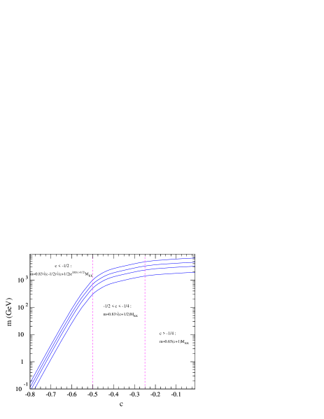
Figure 1: Mass of the lightest ($-+$) KK fermion as a function of $c$ for different values of the KK gauge boson mass. From bottom to top, $M_{KK}=$3, 5, 7, 10 TeV.

As showed above, the $(-+)$ LH KK state is lighter than the gauge KK states for $c<1/2$ (and exponentially light for $c<-1/2$). The KK mode being a Dirac fermion, its Dirac partner with $(+-)$ BC and RH chirality (denoted by “hat”, for example, $\hat{L}^{\prime}$) is also light (since the two helicities obviously have the same spectrum). We can show that the “effective” $c$ (i.e., the $c$ appearing in equations of motion) for the RH helicity is opposite to that of the LH helicity. This implies that the $(+-)$ left-handed KK states (and also their $(-+)$ RH partners) are lighter than the gauge KK states for $c>-1/2$ (exponentially light for $c>1/2$). For instance, we will consider later on a model where $SO(10)$ is broken on the TeV brane in which case left-handed GUT partners of SM fermions (i.e., with same chirality as SM fermions) will have $(+-)$ BC so that LH $(+-)$ KK partners of light SM fermions (which have $c>1/2$) will be exponentially light.

For simplicity, sometimes (as we did in the plot above) we will refer to the LH chirality only (i.e. the same Lorentz helicity as the zero-mode), but it is understood that we mean the Dirac fermion. The consideration of the other chirality of the $(-+)$ fermion gives another intuitive understanding of its lightness as follows. Changing BC on the Planck brane (where $SO(10)$ is broken) from $(++)$ to $(-+)$ adds an extra (RH) $(+-)$ chirality which is localized near the Planck brane for $c\ll 1/2$ since the change of BC is a small perturbation. Then, the small overlap of the two chiralities (the $(-+)$ LH chirality, i.e., would-be-zero-mode is localized near the TeV brane) explains the small mass of the $(-+)$ fermion.

4.2 The LZP is likely to belong to the multiplet containing the SM right-handed top

We have seen that $(-+)$ KK fermions are lighter than gauge KK states for $c<1/2$ so that the LZP is a $(-+)$ fermion from the bulk multiplet having the smallest $c$ provided $c<1/2$ (see Fig. 1). Recall that the smallest c is that of $t_{R}$ (see subsection 2.1). Hence, the LZP comes from the multiplet wich contains the $t_{R}$ zero mode. Moreover, its $c$ can be close to $-1/2$ so that $m_{LZP}\ll$ TeV is possible.

At tree level and before any GUT breaking, all fields within a GUT multiplet have the same $c$. Loop corrections and bulk breaking of the GUT will lift the degeneracy between these KK masses. In the absence of a detailed loop calculation, we are unable to predict the mass spectrum and we will be guided by phenomenological requirements: the LZP should be colorless and electrically neutral if it is to account for dark matter. In Pati-Salam, where the gauge group is $SU(4)_{c}\times SU(2)_{L}\times SU(2)_{R}$, bulk fermions are ${\bf(4,2)}$ of $SU(4)_{c}\times SU(2)_{R}$ and ${\bf(4,2)}$ of $SU(4)_{c}\times SU(2)_{L}$. So the LZP has gauge quantum numbers of a right-handed (RH) lepton doublet since $\tilde{b}_{R}$ is neutral under $Z_{3}$ (tilded fermions denote $SU(2)_{R}$ partners of SM fermions and do not have zero modes). $e^{\prime}_{R}$ can be heavier than $\nu^{\prime}_{R}$ due to electroweak loop corrections to KK masses (primed fermions denote $SU(4)_{c}$ partners and do not have zero modes).

In $SO(10)$, there are additional $Z_{3}$-charged quark-like states in the 16 GUT multiplet containing $t_{R}$. These are probably heavier than $\nu^{\prime}_{R}$ due to QCD loop corrections. Additional $Z_{3}$-charged lepton-like states can again be heavier than $\nu^{\prime}_{R}$ due to electroweak loop corrections. $\nu^{\prime}_{R}$ is actually the only viable dark matter candidate. Indeed, it is well known that TeV left-handed neutrinos are excluded by direct detection experiments because of their large coupling to the $Z$ gauge boson [25]. To ensure that $\nu^{\prime}_{R}$ is the LZP (if electroweak corrections are not enough) we can make use of bulk breaking of the unified gauge group. This easily allows for splitting in $c$’s of the different component of the GUT multiplet (see section 7).

We are now ready to discuss in more details model-building issues. We start with the unified gauge symmetry in the bulk of AdS₅. The gauge group can then be broken on the branes by boundary conditions or in the bulk by giving a vev to a scalar field. As seen previously, we are forced to break the GUT by boundary conditions to prevent proton decay. In addition, we will find it useful to break it also in the bulk by a small amount. For simplicity, we will start with the Pati–Salam model. We will then extend it to $SO(10)$ which can accomodate gauge coupling unification, just like $SU(5)$ as shown in reference [12].

5 Pati-Salam model

In the background of Eq. (1), the lagrangian for our model reads:

$$S=\int d^{4}x\ dz\sqrt{g}\ \left({\cal L}_{gauge}+{\cal L}_{fermion}+{\cal L}_{UV}\ \delta(z-z_{h})+{\cal L}_{IR}\ \delta(z-z_{v})\right)$$ (9)

${\cal L}_{gauge}+{\cal L}_{fermion}$ is the bulk lagrangian. ${\cal L}_{fermion}$ is given in Eq. 3. We now focus on ${\cal L}_{gauge}$:

$${\cal L}_{gauge} = \sqrt{g}\big{(}-\frac{1}{4}Tr{W_{L}}_{MN}W_{L}^{MN}-\frac{1}{4}Tr{W_{R}}_{MN}W_{R}^{MN}$$ (10)

$$-\frac{1}{4}TrF_{MN}F^{MN}+|D_{M}\Sigma|^{2}-V(\Sigma)+\frac{a_{i}}{\Lambda^{3/2}}\Sigma{F_{i}}_{MN}F_{i}^{MN}\big{)}$$

where the indices are contracted with the bulk metric $g_{MN}$. ${W_{L}}_{MN}$, ${W_{R}}_{MN}$ and $F_{MN}$ are the field strengths for, respectively, $SU(2)_{L}$, $SU(2)_{R}$ and $SU(4)_{c}$. $\Sigma$ is a scalar transforming under the Pati-Salam gauge symmetry. Its sole purpose is to spontaneously break Pati-Salam to the SM gauge group at a mass scale below $k$. Specifically, $\langle\Sigma\rangle\equiv v_{\Sigma}^{3/2}$ so that non standard gauge fields acquire a bulk mass $\sim M_{GUT}\sim g_{5D}v_{\Sigma}^{3/2}$. The higher-dimensional operator coupling $\Sigma$ to the gauge fields gives threshold-type corrections to the low-energy gauge couplings (see Eq. 45) and is suppressed by $\Lambda$, the $5D$ cut-off of the RS effective field theory. We will discuss the motivation for this bulk breaking of GUT in section 7.

${\cal L}_{UV}$ includes the necessary fields to spontaneously break $U(1)_{R}\times U(1)_{B-L}$ to $U(1)_{Y}$ on the UV brane and ${\cal L}_{IR}$ contains the SM Higgs field, a bidoublet of $SU(2)_{L}\times SU(2)_{R}$ (there is no Higgs triplet):

$${\cal L}_{IR}={\cal L}_{Higgs}+{\cal L}_{Yukawa},$$ (11)

${\cal L}_{Yukawa}$ generates Yukawa couplings for fermions, it will be given in Eq. 20 and

$${\cal L}_{Higgs}=\sqrt{-g_{IR}}\left(D_{\mu}H\big{[}D^{\mu}H\big{]}^{\dagger}-V(H)\right).$$ (12)

$g_{IR}$ is the induced flat space metric in the IR brane. After the usual field redefinition of $H$ [1], Eq. (12) takes its canonical form:

$${\cal L}_{Higgs}=D_{\mu}H\big{[}D^{\mu}H\big{]}^{\dagger}-V(H)$$ (13)

with $\langle H\rangle=\left(\begin{array}[]{c}0\\ v/\sqrt{2}\end{array}\right)$, $v\approx 250$ GeV.

We assume that brane-localized kinetic terms for bulk fields are of order loop processes involving bulk couplings and are therefore neglected in our analysis.

5.1 Breaking of Pati–Salam on the UV brane

$SU(4)_{c}\times SU(2)_{L}\times SU(2)_{R}$ is first broken to $SU(3)_{c}\times SU(2)_{L}\times U(1)_{R}\times U(1)_{B-L}$ by assigning the following boundary conditions to the $\mu$-components of the gauge fields [17, 18, 19].

$$\begin{array}[t]{ccc}&\textrm{UV}&\textrm{IR}\\ X_{s}&-&+\\ W_{R\;\mu}^{1,2}&-&+\\ \hbox{other gauge fields}&+&+\end{array}$$

This can be done by either orbifold BC or more general BC which approximately correspond to ($-+$) BC. On the other hand, the breaking of $U(1)_{R}\times U(1)_{B-L}\rightarrow U(1)_{Y}$ cannot be achieved by orbifold BC. There are two linear combinations of $W_{R\;\mu}^{3}$ and $V_{\mu}$, where $V_{\mu}$ denotes the $(B-L)$ gauge boson. One, $B_{\mu}$, has ($++$) BC and is the hypercharge gauge boson, whereas the orthogonal combination, denoted by $Z^{\prime}$, is spontaneously broken due to its coupling to a Planckian vev on the UV brane, which mimics $(-+)$ BC to a good approximation.

$$Z^{\prime}_{\mu}\equiv\frac{g_{5\;R}W_{R\;\mu}^{3}-\sqrt{3/2}g_{5\;c}V_{\mu}}{\sqrt{g_{5\;R}^{2}+\left(\sqrt{3/2}\;g_{5\;c}\right)^{2}}}\qquad\qquad B_{\mu}\equiv\frac{\sqrt{3/2}\;g_{5\;c}W_{R\;\mu}^{3}+g_{5\;R}V_{\mu}}{\sqrt{g_{5\;R}^{2}+\left(\sqrt{3/2}\;g_{5\;c}\right)^{2}}}$$ (14)

The electroweak covariant derivative reads

$$D_{M}=\partial_{M}-i(g_{5\;L}W^{a}_{L\;M}\tau_{a\,L}+g_{5\;R}W^{a}_{R\;M}\tau_{a\,R}+\sqrt{3/2}\;g_{5\;c}V_{M}(B-L)/2)$$ (15)

where $g_{5\ c}$, $g_{5\;L}$ and $g_{5\;R}$ are the $5D$ gauge couplings of $SU(4)_{c}$, $SU(2)_{L}$ and $SU(2)_{R}$, respectively and the $\sqrt{3/2}$ factor in the coupling of $V$ comes from $SU(4)_{c}$ normalization. In terms of $Z^{\prime}$ and $B$, the five dimensional electroweak covariant derivative is now

$$D_{M}=\partial_{M}-i\Big{[}g_{5\;L}W_{L\;M}^{a}\tau_{a\,L}+g_{5\;R}W^{1,2}_{R\;M}\tau^{1,2}_{R}+g_{5\;Z^{\prime}}Z^{\prime}_{M}Q_{Z^{\prime}}+g_{5}^{\prime}B_{M}(\tau^{3}_{R}+1/2(B-L))\Big{]}$$ (16)

The couplings of the hypercharge ($Y=\tau_{R}^{3}+(B-L)/2)$ and $Z^{\prime}$ gauge bosons are

$$g^{\prime}_{5}=\frac{\sqrt{3/2}\;g_{5\;c}\;g_{5_{R}}}{\sqrt{g_{5\;R}^{2}+\left(\sqrt{3/2}\;g_{5\;c}\right)^{2}}}\ \ \ ,\ \ \ g_{5\;Z^{\prime}}=\sqrt{g_{5\;R}^{2}+\left(\sqrt{3/2}\;g_{5\;c}\right)^{2}}$$ (17)

Also, the charge under $Z^{\prime}$ and the mixing angle between $V$ and $W_{R}^{3}$ read

$$Q_{Z^{\prime}}=\tau^{3}_{R}-\sin^{2}\theta^{\prime}\;Y,\ \ \ \ \ \ \sin\theta^{\prime}=\frac{\sqrt{3/2}\;g_{5\;c}}{g_{5\;Z^{\prime}}}$$ (18)

5.2 Bulk fermion content

The usual RH fermionic fields are promoted to doublets of $SU(2)_{R}$. Quarks and leptons are unified into the 4 of $SU(4)_{c}$. However, the SM zero modes originate from different multiplets. Indeed, since we are breaking $SU(2)_{R}$ symmetry through the UV orbifold, one component of $SU(2)_{R}$ doublet must be even and have a zero-mode while the other component must be odd and not have a zero-mode. Thus, $u_{R}$ and $d_{R}$ as well as $e_{R}$ and $\nu_{R}$ will have to come from different $SU(2)_{R}$ doublets. Consequently, we are forced to a first doubling of the number of $({\bf 4,2})$’s of $SU(4)_{c}\times SU(2)_{R}$. Since we are also breaking $SU(4)_{c}$ through the UV orbifold, a second doubling is required in such a way that from the ${\bf 4}$ of $SU(4)_{c}$, only the quark must be even and the color singlet must be odd, or vice versa. This is the usual procedure of obtaining quarks and lepton zero-modes from different $SU(5)$ bulk multiplets in orbifolded GUT scenarios [18, 19]. Concerning $({\bf 4,2})$ of $SU(4)_{c}\times SU(2)_{L}$, they are doubled only once, again to split quarks from leptons, i.e., in order to guarantee that $X_{s}$ does not couple SM quarks to SM leptons (just as for $({\bf 4,2})$’s of $SU(4)_{c}\times SU(2)_{R}$ above). To summarize, we have per generation, four types of $({\bf 4,2})$ under $SU(4)_{c}\times SU(2)_{R}$, denoted by $F_{R}$, and two types of $({\bf 4,2})$ under $SU(4)_{c}\times SU(2)_{L}$, denoted by $F_{L}$:

$$F^{q}_{R\;1}=\begin{pmatrix}u_{R}\\ \tilde{d}_{R}\\ e_{R}^{\prime}\\ \nu_{R}^{\prime}\\ \end{pmatrix},\ F^{q}_{R\;2}=\begin{pmatrix}\tilde{u}_{R}\\ d_{R}\\ e_{R}^{\prime}\\ \nu_{R}^{\prime}\\ \end{pmatrix},\ F^{l}_{R\;1}=\begin{pmatrix}u_{R}^{\prime}\\ d_{R}^{\prime}\\ e_{R}\\ \tilde{\nu}_{R}\\ \end{pmatrix},\ F^{l}_{R\;2}=\begin{pmatrix}u_{R}^{\prime}\\ d_{R}^{\prime}\\ \tilde{e}_{R}\\ \nu_{R}\\ \end{pmatrix},\ F^{q}_{L}=\begin{pmatrix}u_{L}\\ d_{L}\\ e^{\prime}_{L}\\ \nu^{\prime}_{L}\\ \end{pmatrix},\ F^{l}_{L}=\begin{pmatrix}u^{\prime}_{L}\\ d^{\prime}_{L}\\ e_{L}\\ \nu_{L}\\ \end{pmatrix}$$ (19)

The untilded and unprimed particles are the ones to have zero modes, i.e. they are $(+,+)$. The extra fields (again, tildes denote $SU(2)_{R}$ partners and primes denote $SU(4)_{c}$ partners) needed to complete all representations are $(-+)$ since breaking of $SU(2)_{R}\times SU(4)_{c}$ is on the Planck brane. Strictly speaking, on an orbifold, $u_{R}$ and $e_{R}$ from the same multiplet (and similarly $d_{R}$ and $\nu_{R}$) are forced to have same BC. So, for example, $e^{\prime}_{R}$ in $F_{R\;1}^{q}$ is $(++)$ to begin with, but we assume that it has a Planckian (Dirac) mass with a Planck brane localized fermion which mimics $(-+)$ BC to a good approximation (a similar assumption holds for $\nu^{\prime}_{R}$ in $F_{R\;2}^{q}$, $u^{\prime}_{R}$ in $F_{R\;1}^{l}$ and $d^{\prime}_{R}$ in $F_{R\;2}^{l}$).

To each $({\bf 4,2})$, we assign the baryon-number corresponding to that of its zero-mode. $U(1)_{B}$ commutes with Pati-Salam and we repeat that it should not be confused with the “$B-L$” subgroup of Pati-Salam. Note that tilded particles are not “exotic” (no $Z_{3}$ charge). Only primed particles carry an exotic baryon number and hence have $Z_{3}$ charge.

As for the Yukawa couplings to the Higgs, they are necessarily localized on the IR brane:

$${\cal L}_{Yukawa}=\sqrt{-g_{IR}}H\left(\lambda_{u\;5}F^{q}_{L}F^{q}_{R\;1}+\lambda_{d\;5}F^{q}_{L}F^{q}_{R\;2}+\lambda_{e\;5}F^{l}_{L}F^{l}_{R\;1}+\lambda_{\nu\;5}F^{l}_{L}F^{l}_{R\;2}\right)$$ (20)

Note that because $u_{R}$ and $d_{R}$ zero-modes arise from different $SU(2)_{R}$ doublets, we are able to give them separate Yukawa couplings without violating $SU(2)_{R}$ on the IR brane.

5.3 On an interval (instead of an orbifold)

If we were to break Pati-Salam to the SM by more general boundary conditions [26], the splitting of the $SU(2)_{R}$ doublet and ${\bf 4}$ of $SU(4)_{c}$ would a priori not be forced by consistency of BC. But, we could not impose baryon-number consistently in a GUT if we do not split $4$ of $SU(4)_{c}$. So, at least, quark/lepton splitting in the ${\bf 4}$ of $SU(4)_{c}$ would be necessary (by assigning Neumann/Dirichlet BC on the Planck brane). The up-down quark isospin splitting could still be achieved (without doubling of representations) for light fermions localized near the Planck brane thanks to different kinetic terms on the Planck brane where $SU(2)_{R}$ is broken. This cannot work for top-bottom since $t_{R}$ has to be localized near the TeV brane where $SU(2)_{R}$ is unbroken and $b_{R}$ is localized near the Planck brane: thus, the splitting of the top/bottom $SU(2)_{R}$ doublet would also be necessary. Whether the splitting of $e_{R}$ and $\nu_{R}$ zero-modes (to obtain different Dirac masses for charged leptons and neutrinos in case Planck brane kinetic terms are not enough to do the splitting) is required by phenomenology depends on the mechanism for generating neutrino masses.

6 Going to $SO(10)$

6.1 Extra gauge bosons, relations between gauge couplings and larger fermion multiplets

When extending the gauge group to $SO(10)$, there are additional gauge bosons, $X$, $Y$, $X^{\prime}$ and $Y^{\prime}$, which are given $(-+)$ BC. The SM Higgs is now contained in $10_{H}$ of $SO(10)$, assigned $B=0$. The breaking of $SO(10)$ to $SO(9)$ by the vev $\langle 10_{H}\rangle$ leads to the existence on the TeV brane of a color triplet pseudo Nambu-Goldstone boson, which will be discussed in the section 7.2.

The previous three gauge couplings are now unified $g_{5c}=g_{5R}=g_{5L}\equiv g_{5}$ with the following relations: $\sin^{2}\theta^{\prime}=3/5$, $g_{5Z^{\prime}}=\sqrt{5/2}\;g_{5}$ and $g^{\prime}_{5}=g_{5}\sqrt{3/5}$ so that $\sin^{2}\theta_{W}=3/8$ at tree level at the GUT scale. Log-enhanced, non-universal loop corrections will modify the relation between the low-energy 4D $g^{\prime}$ and $g$ couplings (just as in the $4D$ SM). The main reason is that the zero-modes can span the entire extra dimension up to the Planck brane where $SO(10)$ is broken and so loops are sensitive to Planckian cut-off’s leading to loop-corrected $\sin^{2}\theta_{W}\approx 0.23$. On the other hand, $\sin^{2}\theta^{\prime}$ appears only in the couplings of KK modes. Those receive very small non-universal loop corrections (universal loop corrections do not modify mixing angles) since KK modes are localized near the TeV brane, where $SO(10)$ is unbroken. Therefore, $\sin^{2}\theta^{\prime}$ is not modified by loop corrections. We will extend this discussion in section 11.1.

For fermions, let us start with the orbifold compactification. In this case, we are forced by the consistency of BC to split not only quarks from leptons and but also $SU(2)_{L}$ and $SU(2)_{R}$ doublets. In addition, we have to split the components of the $SU(2)_{R}$ doublet. Thus, each of the previous $({\bf 4,2})$ of $SU(4)_{c}\times SU(2)_{R}$ and of $SU(4)_{c}\times SU(2)_{L}$ are promoted into a full ${\bf 16}$ of $SO(10)$ with the extra states again assigned $(-+)$ BC. This leads to six ${\bf 16}$’s per generation. Explicitly, one ${\bf 16}$ of $SO(10)$ for each SM representation: $Q_{L}=(u_{L},d_{L})$, $u_{R}$, $d_{R}$, $L_{L}=(e_{L},\nu_{L})$, $e_{R}$ and $\nu_{R}$:

$${\bf 16_{u_{R}}}=\begin{pmatrix}u_{R}\\ \tilde{d}_{R}\\ e_{R}^{\prime}\\ \nu_{R}^{\prime}\\ L^{\prime}_{L}\\ Q^{\prime}_{L}\\ \end{pmatrix},{\bf 16_{d_{R}}}=\begin{pmatrix}\tilde{u}_{R}\\ d_{R}\\ e_{R}^{\prime}\\ \nu_{R}^{\prime}\\ L^{\prime}_{L}\\ Q^{\prime}_{L}\\ \end{pmatrix},{\bf 16_{e_{R}}}=\begin{pmatrix}u_{R}^{\prime}\\ d_{R}^{\prime}\\ e_{R}\\ \tilde{\nu}_{R}\\ L^{\prime}_{L}\\ Q^{\prime}_{L}\\ \end{pmatrix},{\bf 16_{\nu_{R}}}=\begin{pmatrix}u_{R}^{\prime}\\ d_{R}^{\prime}\\ \tilde{e}_{R}\\ \nu_{R}\\ L^{\prime}_{L}\\ Q_{L}^{\prime}\\ \end{pmatrix},{\bf 16_{Q_{L}}}=\begin{pmatrix}Q_{L}\\ L^{\prime}_{L}\\ u^{\prime}_{R}\\ d^{\prime}_{R}\\ e^{\prime}_{R}\\ \nu^{\prime}_{R}\\ \end{pmatrix},{\bf 16_{L_{L}}}=\begin{pmatrix}Q^{\prime}_{L}\\ L_{L}\\ u^{\prime}_{R}\\ d^{\prime}_{R}\\ e^{\prime}_{R}\\ \nu^{\prime}_{R}\end{pmatrix}$$

The last two lines of the first four multiplets (and the last four lines of the last two multiplets) are the extra states in going from $(4,2)$ of Pati-Salam to ${\bf 16}$ of $SO(10)$.

Like in Pati-Salam, breaking $SO(10)$ on an interval (by assigning Dirichlet/Neumann BC for gauge bosons) does not necessarily force us to split fermion multiplets (either quark-lepton splitting, $SU(2)_{L}$–$SU(2)_{R}$ doublet splitting or splitting within a $SU(2)_{R}$ multiplet). But, phenomenologically, like in Pati-Salam, we have to obtain SM quarks and leptons from different ${\bf 16}$’s to suppress proton decay and split $SU(2)_{L}$ and $SU(2)_{R}$ quark doublets to assign baryon number. And again, we also need to split $t_{R}$ and $b_{R}$ in a realistic model. This would lead to three 16’s per generation: one 16 for $SU(2)_{L}$ quark doublet, one for $SU(2)_{R}$ quark doublet and one 16 for leptons, which is what we presented in [20], plus an extra 16 to split $t_{R}$ and $b_{R}$. Imposing lepton number symmetry, as discussed below, further requires to split $SU(2)_{L}$ and $SU(2)_{R}$ lepton doublets. This would amount in thirteen 16’s in total. We will discuss the impact of this large number of representations on the loop corrections to gauge couplings in subsection 11.3.

6.2 Lepton Number Symmetry

Left and right-handed leptons could be obtained from the same ${\bf 16}$ (as we did in our toy example [20]). However, in a realistic model, we are forced to split them for the following reason. If $SO(10)$ is unbroken in the bulk, Majorana masses for SM $\nu_{L}$ cannot be written on the TeV brane since the $L_{L}L_{L}HH$ operator is forbidden by the $B-L$ gauge symmetry (and similarly, bulk Majorana masses, i.e., $\nu_{R}\nu_{R}$ operator for RH neutrinos are not allowed). However, we will break $SO(10)$ in the bulk for reasons presented in section 7. In this case, $B-L$ is also broken in the bulk (in general) and the operator $L_{L}L_{L}HH$ is allowed. This gives Majorana masses for SM $\nu_{L}$ of roughly the same size as charged lepton masses since the effective UV cut-off suppressing this operator is of order TeV, with some, but not much suppression from GUT breaking. In addition, bulk Majorana masses for right-handed neutrinos are also allowed and spoil the seesaw mechanism of reference [27]. In short, lepton-number is violated at low scale. To remedy this problem, we have to impose a bulk gauged lepton-number symmetry in addition to the baryon-number symmetry. We can break it spontaneously on the Planck brane, just like we do with baryon-number which would restrict Majorana masses for $\nu_{R}$ to be written on the Planck brane only, as required for see-saw mechanism for neutrino masses of reference [27].

SM left and right-handed leptons come from different ${\bf 16}$’s with lepton numbers $+1$ and $-1$ and other ${\bf 16}$’s and Higgs are assigned zero lepton-number. For simplicity, the toy example we presented in [20] did not invoke splitting of $SU(2)_{R}$ multiplet nor splitting of left and right-handed leptons.

7 Bulk breaking of unified gauge symmetry

7.1 In Pati-Salam and $SO(10)$

We are willing to invoke the bulk breaking of GUT via the scalar $\Sigma$ (see Eq. 10) in both Pati-Salam and $SO(10)$ for the following reasons:

• The Yukawa coupling $\lambda_{t\;5}Hb_{L}\tilde{b}_{R}$ (see Eq. 20) leads to a mass term of the type $m_{t}b_{L}^{(0)}\tilde{b}_{R}^{(1)}f\left(c_{R}\right)$, where $f(c)\approx\sqrt{2/(1-2c)}$ (for $c>-1/2$) where we used Eq. 30 and the wavefunction of $\tilde{b}_{R}^{(1)}$ given in appendix A.2. There is also a KK mass, $m_{\tilde{b}_{R}^{(1)}}\tilde{b}_{R}^{(1)}\hat{\tilde{b}}^{(1)}_{R}$, where $\hat{\tilde{b}}^{(1)}_{R}$ is the $5D$ KK partner of $\tilde{b}_{R}^{(1)}$. The mixing between $b_{L}^{(0)}$ and $\hat{\tilde{b}}^{(1)}_{R}$ results in a shift in the coupling of $b_{L}$ to $Z$ of order $\sim m_{t}^{2}f\left(c_{R}\right)^{2}/m^{2}_{\tilde{b}_{R}^{(1)}}$, using $f\left(c_{R}\right)\sim 1$ (the analysis is similar to the $\nu^{\prime}_{R}-\nu^{\prime}_{L}$ mixing in section 9.3). For this shift to be $\lesssim 1\%$, $\tilde{b}_{R}^{(1)}$ needs to be heavier than $\sim 1.5$ TeV, meaning that the $c$ for $b^{\prime}_{R}$ should be $\gtrsim-1/4$ if the gauge KK mass $M_{KK}\approx$ 3 TeV (see spectrum in section A.2). In the absence of bulk breaking, the $c$’s for all components of $t_{R}$ multiplet are the same and $\nu^{\prime}_{R}$ will have to be heavier than $\sim 1.5$ TeV also which restricts the viable parameter space for the LZP to account for dark matter.

• As mentioned above, we want to ensure that $e^{\prime}_{R}$ in Pati-Salam (and other lepton-like states in $SO(10)$) is heavier than $\nu^{\prime}_{R}$ in case electroweak corrections were not large enough to achieve the required splitting. A small amount of bulk breaking of $SU(2)_{R}$ and Pati-Salam allows us to split the $c$’s of the $(-+)$ fermions in $t_{R}$ multiplet and thus to address the above two issues. To be precise, choose $c$ for $\nu^{\prime}_{R}$ to be smaller than that of $\tilde{b}_{R}$ and $e^{\prime}_{R}$. We will give details on the size of splitting in $c$’s in section 7.5.

• Bulk breaking of $SU(2)_{R}$ is also used to get a contribution to the Peskin-Takeuchi $T$ parameter of order $\sim 0.3$ as required to fit electroweak data [14]: $T_{bulk}\sim\frac{1}{2}\;M_{GUT}^{2}/k^{2}$, where $M_{GUT}$ is the bulk mass of $W_{R}^{\pm}$. If $M_{GUT}/k\sim 1/2$, then $T_{bulk}\sim 0.1$. Loop effects can generate the remaining contribution to $T$ [14]. If $M_{GUT}\sim k$, we get a too large $T_{bulk}\sim 0.5$ – this is another reason, independent of unification considerations in $SO(10)$ (see section 7.5), to assume that $M_{GUT}<k$.

7.2 Specificities of $SO(10)$

In $SO(10)$ there are additional reasons to invoke bulk breaking:

• To achieve gauge coupling unification [12] (see section 11).

• To make the Higgs triplet, charged under $Z_{3}$, heavier than $\nu^{\prime}_{R}$. Indeed, we do not want it to be the LZP. As a colored particle, it is not a suitable dark matter candidate. Without bulk breaking and at tree-level, it is the massless (pseudo) Nambu-Goldstone boson coming from the breaking of $SO(10)$ to $SO(9)$ by the Higgs vev (recall that BC’s on the TeV brane do not break $SO(10$)). $SO(10)$ being broken also on the Planck brane (by BC), loop corrections will give it a mass which may be too small, of order $\alpha_{s}M_{KK}^{2}/\pi$. With bulk breaking, the Higgs triplet gets a tree-level mass via the operator $\Sigma{\bf 10}_{H}{\bf 10}_{H}$. For sufficient bulk GUT breaking, this mass is larger than the one-loop induced mass so that Higgs triplet can be heavier than $\nu^{\prime}_{R}$.

• To make some $Z_{3}$-charged particles such as $X$, $X^{\prime}$, $Y$, $Y^{\prime}$ or $Q^{\prime}_{L},L_{L}^{\prime}$ from the multiplet with $t_{R}^{(0)}$ or $\nu^{\prime}_{R}$, $u^{\prime}_{R}$ from the multiplet with $Q_{L}^{(0)}$, decay before Big Bang Nucleosynthesis (BBN). In the absence of bulk breaking, they can only decay via very higher-dimensional operators so that their decay width may be too small, as explained in the next section. Note that (non-SM) Pati-Salam gauge boson ($X_{s}$) and Pati-Salam partners of zero-mode fermions decay easily as mentioned below.

7.3 Decay of KK particles (other than the LZP)

Clearly, $Z_{3}$-charged particles eventually decay into the LZP. In Pati–Salam, $Z_{3}$ charged particles decay into $\nu^{\prime}_{R}$ easily: $e^{\prime}_{R}$ from $t_{R}^{(0)}$ multiplet decays into LZP $+W^{\pm}_{R}$, followed by $W^{\pm}_{R}$ mixing with $W_{L}^{\pm}$ zero-mode due to EW symmetry breaking: the coupling $e^{\prime}_{R}W^{\pm}$ LZP is similar to the coupling of the LZP to $Z$ induced via $Z-Z^{\prime}$ mixing after EW symmetry breaking (see section 9.2), of order $\sim gk\pi r_{c}m_{W}^{2}/M_{KK}^{2}\sim g/30$ for $M_{KK}\sim 3$ TeV. $X_{s}$ decays fast into $t_{R}^{(0)}$ and $\nu^{\prime}_{R}$. $Z_{3}$ charged fermions from other multiplets can decay into the zero-mode from that multiplet and virtual $X_{s}$: for example, $u^{\prime}_{R}$ from multiplet with $e^{(0)}_{R}$ decays into $\tilde{\nu}_{R}+X_{s}$ followed by decays of $X_{s}$ and $\tilde{\nu}_{R}\rightarrow W^{\pm}e^{(0)}_{R}$ (the last decay occurs via $W^{\pm}_{R}-W_{L}^{\mp}$ mixing).

Finally, tilded particles, not charged under $Z_{3}$, decay into their $SU(2)_{R}$ partners which have zero-modes and KK mode $W^{\pm}_{R}$ which again mixes with zero-mode of $W_{L}^{\pm}$. Tilded particles can also decay into $SU(2)_{L}$ doublet and Higgs as follows. As mentioned before (section 7.1), there is a Yukawa coupling $\lambda_{t}f(c_{t_{R}})H\tilde{b}_{R}(t,b)_{L}$ which results in the decay $\tilde{b}_{R}\rightarrow b_{L}H^{0},t_{L}W^{+}_{long.}$ – this dominates over the decay into $t_{R}W^{+}$ (which is suppressed by $W_{R}^{\pm}-W_{L}^{\mp}$ mixing).

In contrast with Pati–Salam, decays in $SO(10)$ of the non-Pati-Salam $Z_{3}$-charged particles (both fermions and gauge bosons) into $\nu^{\prime}_{R}$ are problematic in the absence of bulk breaking. Indeed, there is no short path for this decay. Specifically, $X$, $X^{\prime}$, $Y$, $Y^{\prime}$ or $Q_{L}^{\prime}$ and $L_{L}^{\prime}$ from $t_{R}^{(0)}$ multiplet cannot decay into the LZP via gauge interactions. The reason is that, while there are $t_{R}^{(0)}-X-Q^{\prime}_{L}$ and $t_{R}^{(0)}X^{\prime}L_{L}^{\prime}$ couplings, there are no $t_{R}^{(0)}-X_{s}-Q^{\prime}_{L}$ (or $L^{\prime}_{L})$ couplings and also no $t_{R}^{(0)}-LZP-X$ or $X^{\prime}$ couplings.

Thus, the decays of these particles have to go through higher-dimensional operators, and, in order for these operators not to be suppressed by the Planck scale, they have to be $B$-conserving. For example, operators such as $\left(Q^{\prime}_{L}Q_{L}Q_{L}L\right)\nu^{\prime\;c}_{R}LH$ and $\left(L_{L}^{\prime}Qd^{c}_{R}\nu^{c}_{R}\right)\nu^{\prime}_{R}\bar{L}H$ from $\left({\bf 16}^{4}\right)\times\left({\bf 16}{\bf 16}{\bf 10_{H}}\right)$ will lead to decays of $Q^{\prime}_{L}$ and $L^{\prime}_{L}$ into LZP. They break the usual lepton-number, but do not generate Majorana masses since $L_{L}L_{L}HH$ on the TeV brane or $\nu_{R}\nu_{R}$ in the bulk are forbidden by the unbroken bulk $B-L$ gauge symmetry. Thus, in the absence of bulk breaking, we do not need to impose lepton number to forbid these masses. However, these operators result in $5$-body decays of $Q^{\prime}_{L}$ and $L^{\prime}_{L}$ into LZP with amplitude suppressed by $6$ powers of the KK mass since it is a dimension-$10$ operator and can result in lifetimes longer than the BBN epoch.

Let us give an estimate for the decay width: $\Gamma\sim v^{2}(\Delta m)^{11}/\Lambda^{12}/\left(4096\;\pi^{7}\right)$, where $\Delta m$ is the mass splitting between $Q^{\prime}_{L}$ and the LZP which is small since they have the same $c$, $4096\;\pi^{7}$ comes from the $5$-body phase-space and $\Lambda$ here is the warped-down string scale of order a few TeV. For $\Delta m\sim 0.2\,m_{LZP}\sim 100$ GeV and $\Lambda\sim 3$ TeV, we get $\Gamma\sim 10^{-22}$ GeV and a lifetime of $\sim 10^{-2}$ sec. However, the lifetime is extremely sensitive to $\Delta m$ and $\Lambda$: for example, with $\Delta m\sim 10$ GeV, we get a lifetime of $\sim 10^{9}$ sec. Similarly, decays of $\nu^{\prime}_{R}$ and $u^{\prime}_{R}$ from the multiplet with $Q^{(0)}_{L}$ might be suppressed: their masses are $\sim$ few TeV so that phase-space suppression is smaller (i.e., $\Delta m$ is larger), but still the decay can occur after BBN since, for example, $\Lambda$ can be larger.

Let us now recall why there is a potential danger from late decays of TeV mass particles. Particles decaying after BBN can ruin successful predictions of abundances of light elements. Decay products inject photons and electrons into the plasma which can dissociate light elements. This leads to a lifetime dependent bound on the quantity $m\times Y$, where $m$ is the mass of the decaying particle and $Y=n/s$, where $n$ is the number density that this particle would have today if it had not decayed and $s$ is the entropy density today. The strongest bound is for lifetimes of the order of $10^{8}$s and reads $m\times Y<10^{-12}$ GeV [28]. The standard relic density calculation of cold massive particles leads to

$$m\times Y\sim\frac{x_{F}\sqrt{45}}{\sqrt{\pi g_{*}}M_{Pl}\langle\sigma v\rangle}\sim 3\times 10^{-19}\frac{x_{F}}{\sqrt{g_{*}}\langle\sigma v\rangle}\ \ \mbox{GeV}^{-1}$$ (21)

For a relic behaving as a WIMP, we expect $x_{F}\sim 25$. If it accounts for dark matter then $\langle\sigma v\rangle\sim 10^{-9}$ GeV^-2 and $m\times Y\sim 7.5\times 10^{-9}$ GeV. We see that even if the light KK states we are considering contributed to the final energy density of dark matter by only one percent or one per mil (after they decay into the LZP), they could be dangerous if they decay late, i.e. after BBN. To suppress any potential danger coming from the late decay of these next-to-lightest $Z_{3}$ charged particles (NLZP), we invoke bulk breaking of $SO(10)$ which we discuss next.

7.4 Decays of NLZP’s with bulk breaking of $SO(10)$

In the presence of $SO(10)$ bulk breaking, decays of $Q^{\prime}_{L}$ and $L_{L}^{\prime}$ from the $t_{R}$ multiplet into the LZP easily take place thanks to $X^{\prime}-X_{s}$ and $Y-Y^{\prime}$ mixing due to

$${\cal L}_{IR} \ni \sqrt{-g_{IR}}\left(\frac{b}{M_{S}^{2}}\langle 16_{\Sigma}\rangle D^{\mu}\langle 16_{\Sigma}\rangle D_{\mu}\langle 10_{H}\rangle+D^{\mu}\langle 10_{H}\rangle D_{\mu}\langle 10_{H}\rangle\right)$$ (22)

where $\langle 16_{\Sigma}\rangle$ is in SM singlet component and the covariant derivatives give gauge fields, $X$, $X^{\prime}$ and $X_{s}$. The first term leads to $X^{\prime}-X_{s}$ mixing and hence to the decays

$$t_{L}^{\prime} \rightarrow X^{\prime}\nu^{\prime}_{R}\stackrel{{\scriptstyle\hbox{\tiny{via mixing}}}}{{\rightarrow}}t_{R}^{(0)}\overline{\nu}^{\prime}_{R}\nu^{\prime}_{R}\;\;\ \ \mbox{and}\ \ \nu^{\prime}_{L}\rightarrow{X^{\prime}}^{*}t_{R}^{(0)}\stackrel{{\scriptstyle\hbox{\tiny{via mixing}}}}{{\rightarrow}}t_{R}^{(0)}\bar{t}_{R}^{(0)}\nu^{\prime}_{R}$$

whereas their $SU(2)_{L}$ partners decay as ($X$, $Y$ and $Y^{\prime}$ cannot mix with $X_{s}$ due to their different electric charge)

$$b_{L}^{\prime} \rightarrow t_{L}^{\prime}W_{L}^{-}\rightarrow t_{R}^{(0)}\overline{\nu}^{\prime}_{R}\nu^{\prime}_{R}W^{-}_{L}$$

$$\tau_{L}^{\prime} \rightarrow \nu^{\prime}_{L}W_{L}^{\pm}$$ (23)

$$\rightarrow \nu^{\prime}_{R}t^{(0)}_{R}\bar{t}_{R}^{(0)}W_{L}^{\pm}$$

Similarly, the 2nd term in Eq. (22) gives $Y-{Y^{\prime}}^{*}$ mixing resulting in other decay chains (using the $Y^{\prime}-X^{\prime}-W_{L}$ coupling). We can estimate these decay widths as follows. Naive dimensional analysis (NDA) size for $b$ is $\sim\lambda_{5}\Lambda$ (as expected since it is a coupling of Higgs) resulting in a $X_{s}-X^{\prime}$ mixing term of order $\sim M_{GUT}^{2}\left(\lambda_{5}kv\right)/\Lambda$, where $M_{GUT}$ and $\Lambda$ are actually the warped-down values since this operator is on the TeV brane. We used the fact that wavefunctions for gauge KK modes at the TeV brane are $\sim\sqrt{k}$ (see appendix A.1). Using Eq. 30, we get $\lambda_{5}kv\sim 500$ GeV with $c$ for $(t,b)_{L}\sim 0.4$ and $c$ for $t_{R}\sim-1/2$. Then, the coefficient of the $4$-fermion operator for the decay of, say, $\nu^{\prime}_{L}$, is $\sim g_{\mbox{\tiny SM}}^{2}k\pi r_{c}M_{KK}^{4}\times(X^{\prime}-X_{s}$) mixing. We used the fact that the couplings of the gauge KK mode to KK fermions and $t_{R}^{(0)}$ are enhanced by $\sim\sqrt{k\pi r_{c}}$ compared to $g_{\mbox{\tiny SM }}$ (see section 9.1). Assuming $m_{\nu^{\prime}_{L}}>2m_{t}+m_{LZP}$, we obtain $\Gamma\sim$ (above coefficient)${}^{2}\times$ $\left(m_{\nu^{\prime}_{L}}-2m_{t}-m_{LZP}\right)^{5}/\left(64\pi^{3}\right)$, where $64\pi^{3}$ is from the $3$-body phase-space. For $g_{SM}\sim 1/2$, $m_{\nu^{\prime}_{L}}\sim 1$ TeV and $m_{LZP}\sim 200$ GeV, $M_{GUT}/k\sim 1/2$ we get $\Gamma\sim 10^{-8}$ GeV and a lifetime $\sim 10^{-17}$ sec.

Similarly, $\nu^{\prime}_{R}$ and $u^{\prime}_{R}$ from the multiplet with $Q^{(0)}_{L}$ can decay into $Q^{(0)}_{L}$ + ($X^{\prime},Y^{\prime}$) or ($X$,$Y$), followed by mixing with $X_{s}$. $\nu^{\prime}_{R}$ and $u^{\prime}_{R}$ have masses of a few TeV so that their lifetimes are even shorter than above.

7.5 Size of bulk breaking and splitting in $c$

Having seen the motivation for bulk breaking, we now show what is its natural size. The splitting in $c$ (due to last term of Eq. 3) is given by $(k\Delta c)\sim a^{\prime}\langle\Sigma\rangle/\sqrt{\Lambda}$ (where $a^{\prime}$ is defined in Eq. 3). The NDA sizes for coupling of $\Sigma$ to gauge fields (see Eq. 10) and fermions are $a\sim a^{\prime}\sim g_{5}\sqrt{\Lambda}$ leading to $\Delta c\sim g_{5}v_{\Sigma}^{3/2}/k$. We previously saw that the bulk mass for $X,Y$ is $M_{GUT}\sim g_{5}v_{\Sigma}^{3/2}$ so that

$$\Delta c \sim {M_{GUT}}/{k}.$$ (24)

The size of ${M_{GUT}}/{k}$ can be inferred from the requirement of gauge coupling unification: NDA size for the bulk threshold correction $\Delta$ in $1/g_{4D}^{2}$ (see Eq. 45), from the higher-dimensional operator in Eq. (10) is $\sim k\pi r_{c}/g_{5}^{2}\times M_{GUT}/\Lambda$. The size of this correction should be $\sim 20\%$ (and not larger) to accomodate unification [12]. Using $k\pi r_{c}/g_{5}^{2}\sim 1/g_{4D}^{2}\sim O(1)$, we get $M_{GUT}/\Lambda\sim 1/5$. Of course, this argument is not valid for Pati-Salam. The splitting in $c$ is then given by $\Delta c\sim(1/5)\times\Lambda/k$ where $\Lambda>k$ is required for calculability. We also require that $M_{GUT}/k<1/2$ so that we can use the small GUT breaking approximation as follows. There are one-loop non-universal corrections to $1/g_{4D}^{2}$ (see Eq. 45) from GUT-scale splittings in masses. For example, the splitting between (mass)² of $X,Y$ gauge bosons and SM KK gauge bosons is $O\left(M_{GUT}^{2}/k^{2}\right)$ so that these one-loop corrections have a size $\sim C\;\frac{M_{GUT}^{2}}{k^{2}}\;\frac{k\pi r_{c}}{8\pi^{2}}$, where $C$ is the Dynkin index of the bulk $X/Y$ gauge fields [12]. For $M_{GUT}/k\sim 1/2$, these result in $\Delta_{i}$’s $\sim C/8$ which is about what we require for unification. Whereas, for $M_{GUT}\sim k$, $\Delta_{i}$’s $\sim C/2$ which spoils unification – to repeat, we tolerate $\Delta\sim 1/5$. Combining the above two arguments, we get

$$0.2 \lesssim\Delta c \lesssim 1/2$$ (25)

This size is enough to obtain the splitting in mass between KK particles from the $t_{R}$ multiplet as required in section 7.1. Explicitly, $c$ for GUT partners of $t_{R}$ is given by $c_{t_{R}}\pm\Delta c$ with $c_{t_{R}}\lesssim 0$ and we have seen that the mass of the $(-+)$ fermion is very sensitive to $c$ for $c\sim-1/2$. Thus, $\nu^{\prime}_{R}$ (assuming its $c$ is the smallest) can be significantly lighter than other $Z_{3}$-charged GUT partners of $t_{R}$ and ensured to be the LZP. Also, $\tilde{b}_{R}$ can be easily heavier than $1.5$ TeV (as constrained experimentally by $Z\rightarrow b\bar{b}$), while at the same time $m_{\nu^{\prime}_{R}}<$ TeV (which is the preferred mass range in order to obtain the correct relic density).

8 Other models

Before discussing the interactions of the LZP and showing that it is a good DM candidate, we briefly mention other related models.

8.1 $SO(10)$ breaking on the TeV brane

An alternative possibility is to break $SO(10)$ to $SU(3)\times SU(2)_{L}\times SU(2)_{R}\times U(1)_{B-L}$ on the TeV brane, using $(+-)$ boundary conditions for the other gauge fields of $SO(10)$: we choose not to break $SU(2)_{R}$ by BC on the TeV brane in order to preserve the custodial symmetry. Thus, $SU(2)_{R}\times U(1)_{B-L}$ should be broken to $U(1)_{Y}$ on the UV brane (as in the previous model). Extra fermionic states with the same chirality as zero-modes (i.e., SM fermions) are also $(+-)$ while they are $(-+)$ for the other chirality. We can still define a $Z_{3}$ as before. The LZP now comes from the multiplet with the largest $c$, namely the multiplet with one of the light fermions having $c>1/2$ as explained in section 4.1. As usual, due to bulk GUT breaking, we can assume that the LZP is $\nu^{\prime}_{R}$. Annihilation of the LZP via $Z^{\prime}$ exchange (for $(-+)$ chirality), which will be described in the next section, is the same in the two models. However, the one via $X_{s}$-exchange is negligible in this model since the zero-mode which couples to the LZP via $X_{s}$ is now localized near the UV brane (cf. the previous model, where this channel is important since $t_{R}$ is localized close to the TeV brane). Concerning the coupling of the LZP to the $Z$ (playing an important role in annihilation and elastic scattering and which will be described in the next section), the one occurring via $Z^{\prime}-Z$ mixing (for $(-+)$ chirality) is the same in the two models and the one via $\nu^{\prime}_{R}-\nu^{\prime}_{L}$ mixing (for $(-+)$ chirality) is also similar, except that the $5D$ Yukawa entering this coupling is that of the light fermion.

The Higgs multiplet is still a bi-doublet of $SU(2)_{L}\times SU(2)_{R}$ but there is no Higgs triplet since $SO(10)$ is broken on the TeV brane. As far as unification of couplings goes, if there is no bulk GUT breaking, the “would-be” zero-modes of $X,X_{s}$ etc. get a mass $\sim M_{KK}/\sqrt{k\pi r_{c}}$ which spoils unification. However, with bulk breaking, these modes get a mass of $\sim M_{GUT}$ so that unification is similar to the previous model (see reference [12]).

8.2 Warped SUSY $SO(10)$

If the model has supersymmetry in the bulk, the Higgs can be localized near the Planck brane since SUSY protects its mass. Thus, SM fermions can also be localized very close to the Planck brane ($c\gg 1/2$) so that higher-dimensional baryon-number violating operators are suppressed by Planckian scales. There is no longer a need to impose baryon-number symmetry. There will be no stable KK state. However, there is still a possibility to account for dark matter if the lightest supersymmetric particle is stable via R-parity conservation. Of course, one loses the explanation of the hierarchy of fermion masses which is one of the appealing features of non-SUSY RS. One has to introduce small Yukawa couplings by hand. If one was to address the issue of Yukawa hierarchy by delocalizing the fermions ($c\stackrel{{\scriptstyle<}}{{\sim}}1/2$), then a baryon number symmetry would be required. In addition, the Higgs would also have to be in the bulk and should be given almost a flat profile. Otherwise, MSSM unification will be spoiled by the modification of the contribution of the Higgs to the running. For recent works on warped supersymmetric $SO(10)$, see references [29].

8.3 $SU(5)$ model

$SU(5)$ models do not contain a custodial symmetry and are constrained by EW precision tests. The IR scale has to be pushed to 10 TeV or more (depending on the size of brane kinetic terms). This introduces a little hierarchy problem and also make these models less appealing since there is no hope to produce KK modes at colliders. Nevertheless, we briefly discuss this model to see whether there can be a stable KK particle. Suppose $SU(5)$ is broken to the SM on the Planck brane: $X,Y$ gauge bosons are $(-+)$. If $d_{R}$ from ${\bf\bar{5}}$ is $(++)$, i.e., has zero-mode, then, on an orbifold, $L^{\prime}_{L}$ from the same multiplet has to be $(-+)$. Consistency of BC on an orbifold requires the same BC for $u_{R}$ and $e_{R}$, i.e., zero-modes for both $u_{R}$ and $e_{R}$ can come from the same ${\bf 10}$, but we give one of them a Planckian mass with fermion localized on the Planck brane so that it is effectively $(-+)$. So one gets two ${\bf\bar{5}}$’s and three ${\bf 10}$’s per generation with zero-modes for $d_{R}$, $L_{L}$, $Q_{L}$, $u_{R}$ and $e_{R}$, respectively. One has to impose baryon-number. $Z_{3}$ again gives a stable particle. The only electrically and color neutral,but $Z_{3}$-charged particle is $\nu^{\prime}_{L}$: if it is to account for dark matter, then its mass is constrained to be at least a few tens of TeV from direct detection experiments [25].

On an orbifold, it is also possible to obtain the stability of a KK state via a discrete symmetry not related to baryon-number: One can define $P=Z_{2}$-charge $\times Z_{2}^{\prime}$-charge. Bulk interactions are $P$-invariant even after compactification (which breaks $Z_{2}$ and $Z_{2}^{\prime}$ separately but leave the product intact). Particles with zero-modes $(++)$ are $P$-even, particles with no zero-modes $(-+)$ or $(+-)$ are $P$-odd.

If we assume that the bare lagrangian on each brane respects both $Z_{2}$ and $Z_{2}^{\prime}$ (of course, on an orbifold, it has to respect $Z_{2}$ corresponding to reflection about that brane), then all tree-interactions are $P$-even. Loops cannot generate $P$-violating interactions and P-parity is exact at loop-order. The lightest $P$-odd particle is stable since it cannot decay into $P$-even SM particles hence can be the DM. Again, the only candidate is $\nu^{\prime}_{L}$. Note that in Pati-Salam or $SO(10)$, we cannot assume $P$-parity since the bi-doublet Higgs couples $W_{R}^{\pm}$ $(-+)$ to $W_{L}^{\pm}$ $(++)$, i.e., the Higgs couplings do not preserve $P$-parity.

8.4 $SO(10)$ model with gauged lepton number

As we said in the introduction, imposing only a (gauged) lepton number symmetry is enough to prevent proton decay, although $\Delta B=2$, i.e neutron-antineutron oscillations are still allowed but suppressed by the TeV scale. In this case, we need again to replicate representations. On an interval, three 16’s per generation with lepton numbers $+1$, $-1$ and $0$ containing zero-modes for $L_{L}$ and $L_{R}$ and all quarks, respectively, are sufficient. In addition, extra 16’s for the third generation are needed to split $b_{R}$ and $t_{R}$ as usual and also $(t,b)_{L}$ from $t_{R}$ and $b_{R}$ (due to the three different $c$’s). As in the case of baryon-number symmetry, we add spectators on the Planck brane and break lepton-number spontaneously on that brane.

In this alternative, we do not obtain a stable particle hence no DM candidate. This is because there is no unbroken gauge symmetry under which only leptons are charged so that there is no analog of unbroken $Z_{3}$ symmetry, even if lepton number is unbroken. The $\nu^{\prime}_{R}$ (and other KK states) from $t_{R}$ multiplet will still be light, but $\nu^{\prime}_{R}\rightarrow$ neutron $+S$ (where $S$ is a neutral scalar SM final state with zero lepton number) or proton $+S^{\prime}$ (where $S^{\prime}$ is a charged scalar final state) is allowed. Note that the above decay of $\nu^{\prime}_{R}$ breaks baryon-number by $1$ (since $\nu^{\prime}_{R}$ has zero baryon-number), but this is allowed since we are not imposing baryon-number in this case. The final state has to involve a proton or a neutron which are the only SM fermionic states carrying zero lepton-number (recall that $\nu^{\prime}_{R}$ has zero lepton number). For example, there is a coupling $\left(X^{\prime},Y^{\prime}\right)Q^{(0)}d^{(0)}_{R}$ from a bulk interaction since zero-modes of $Q$ and $d_{R}$ can be obtained form same multiplet so that we get $\nu^{\prime}_{R}\rightarrow t^{(0)}_{R}X_{s}^{*}$, followed by $X_{s}\rightarrow d_{L}^{(0)}d^{(0)}_{R}$ (via $X^{\prime}-X_{s}$ mixing). In this model, baryon number violating decays such as $\left(X^{\prime},Y^{\prime}\right)\rightarrow Q^{(0)}d_{R}^{(0)}$ and $\left(X,Y\right)\rightarrow Q^{(0)}u_{R}^{(0)}$ could be observed at colliders.

However, on an orbifold, consistency of BC will force us to split $SU(2)_{L}$ and $SU(2)_{R}$ doublet quarks also so that we will require a larger number of 16’s. Recall that there is a GUT parity in the bulk in this case (we call it P-parity in section 8.3) under which all $(-+)$ states (with no zero-modes) are odd. Hence, the lightest P-odd state (most likely $\nu^{\prime}_{R}$) cannot decay via bulk interactions. Other light KK states can decay into it in the bulk as in our model with baryon-number. P-parity can be broken by brane interactions. In fact, in $SO(10)$ or Pati-Salam model, Higgs couplings are not invariant under P-parity so that $P$-parity has to be broken on the TeV brane. Thus, $\nu^{\prime}_{R}$ will decay via interactions on the TeV brane. To be concrete, the operator $\bar{16}_{Q}D\!\!\!\!\!\!\!\not\;\;16_{d}$, leading to $\left(X^{\prime},Y^{\prime}\right)\rightarrow Q^{(0)}d_{R}^{(0)}$ as before, is allowed only on the TeV brane. Then, $\nu^{\prime}_{R}$ can decay as before. Or, in the absence of $X^{\prime}-X_{s}$ mixing, $\nu^{\prime}_{R}$ can decay via higher-dimensional operators on the TeV brane.

9 Interactions of the KK right-handed neutrino

We are interested in computing the energy density stored in the LZP. The LZP, once it stops interacting with the rest of the thermal bath, is left as a relic. We define $x_{F}=m/T_{F}$ where $T_{F}$ is the freeze-out temperature. The general formula for the contribution of a massive cold relic to the energy density of the universe is:

$$\Omega_{relic}h^{2}=\frac{s_{0}\ h^{2}}{\rho_{c}M_{Pl}}\sqrt{\frac{45}{\pi g_{*}}}\frac{1}{\int_{x_{F}}^{\infty}dx\ \frac{\langle\sigma v\rangle}{x^{2}}}$$ (26)

Here, $s_{0}$ is the entropy density today, $\rho_{c}$ is the critical energy density of the universe, $h$ is the reduced expansion rate ($H_{0}=h\times 100$ km s^-1 Mpc^-1) and $g_{*}$, the number of relativistic degrees of freedom, is evaluated at the freeze-out temperature. In the non relativistic limit, the thermally averaged annihilation cross section reads $\langle\sigma v\rangle\approx a+bv^{2}$, where $v$ is the relative velocity between the two annihilating particles and Eq. (26) becomes

$$\Omega_{relic}h^{2}=\frac{1.04\times 10^{9}}{M_{Pl}}\frac{x_{F}}{\sqrt{g_{*}}}\frac{\mbox{GeV}^{-1}}{(a+3b/x_{F})}$$ (27)

where $a$ and $b$ are in GeV^-2. In the industriously studied case of neutralino dark matter, $a$ is smaller than $b$ because of the Majorana nature of the dark matter particle, leading to a $p$-wave suppression of the annihilation cross section. In contrast, the LZP is a Dirac fermion and its cross section is not helicity suppressed. To evaluate $\Omega_{LZP}$, we need to compute the annihilation cross section of the LZP. By definition, a WIMP has an annihilation cross section of the right order, $10^{-9}$ GeV^-2, leading to the appropriate relic density to account for dark matter. We will now detail how our KK right-handed neutrino annihilates and explain why we expect it to behave as a typical WIMP.

9.1 Estimates of cross-sections

We start with estimates of the couplings of the LZP and of its annihilation and elastic scattering cross-sections. We will then present the details in the following sections and appendices.

All gauge and fermion KK modes, including the LZP, as well as the Higgs, the top and possibly the left-handed bottom quarks, are localized near the TeV brane. Consequently, any coupling between these particles is large. The LZP can annihilate significantly through an $s$-channel exchange of $Z^{\prime}$ gauge boson (into top quarks and Higgs) as well as a $t$-channel exchange of KK $X_{s}$ gauge boson into a zero mode $t_{R}$ as shown in Fig. 2 (recall that the LZP is from the $t_{R}$ multiplet). As explained below, those couplings are typically 5 or 6 times larger than SM couplings. However, the particle which is exchanged has a mass of at least 3 TeV. Effectively, the annihilation cross section has the same size as the one involving SM couplings and particles of mass of order 500 GeV. We are indeed dealing with “weak scale” annihilation cross sections.

In addition, we will show that the LZP has a significant coupling to the $Z$. Since the LZP can be naturally much lighter than gauge KK modes, $s$-channel annihilation through $Z$-exchange can also have the right size. This coupling also results in a cross-section for direct detection via $t$-channel $Z$ exchange which is of weak-scale size.

We explain in appendix E why we can neglect the annihilation through Higgs exchange in our analysis.

Note that at the lowest order, the LZP cannot annihilate with itself into SM particles but only with its antiparticle, due to $Z_{3}$ conservation.

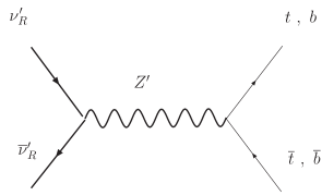
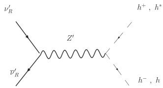
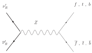
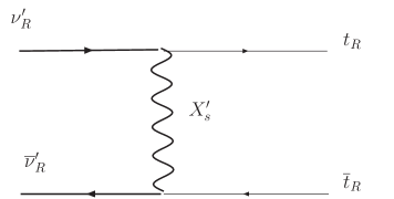
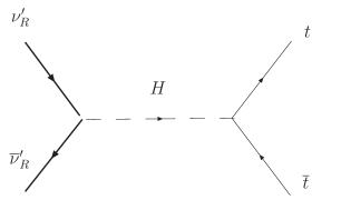
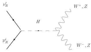
Figure 2: LZP annihilation channels. $f$ denotes all SM fermions other than top and bottom.

Let us begin by estimating the couplings of the LZP. The $\nu^{\prime}_{R}X_{s}t_{R}^{(0)}$ coupling, appearing in the $t$-channel annihilation, is given by the overlap of the three wavefunctions (see Eq. 100). The coupling of $\nu^{\prime}_{R}$ to $Z^{\prime}$ KK modes, used in the s-channel $Z^{\prime}$ annihilation, is given by Eq. 99. Using the wavefunctions in Eqs. 78, 79 and 90, we can show that $t_{R}^{0}$, $Z^{\prime}$ and $X_{s}$ KK modes and $(-+)$ helicity of the LZP are all localized near the TeV brane. So, we expect the above couplings of the LZP (for $(-+)$ helicity) to have the same size as the coupling of, say, gauge KK modes to the Higgs on the TeV brane. Evaluating the wavefunction of the gauge KK mode (see Eq. 79) at the TeV brane, we can show that the coupling of the gauge KK mode to the Higgs is enhanced compared to that of zero-mode gauge bosons by $\approx\sqrt{2k\pi r_{c}}$ so that we expect the above two couplings to be also $\sim\sqrt{k\pi r_{c}}\times$ $4D$/zero-mode gauge coupling. A numerical evaluation of the overlaps Eqs. (100) and (99) indeed confirms this expectation. This is also expected from the CFT interpretation as explained in section F.4. For $c\lesssim-1/2$, the coupling of the other $(+-)$ helicity of the LZP to $X_{s}$ and $Z^{\prime}$ is suppressed since it is localized near the Planck brane (see appendix A.2).

As mentioned above, the coupling of $Z^{\prime}$ to the Higgs is enhanced compared to SM couplings (see also Eq. 89). Similarly, the coupling of $t_{R}$ to $Z^{\prime}$ is also enhanced by $\sqrt{k\pi r_{c}}$ compared to $4D$ (“would-be” zero-mode) gauge coupling since both $t_{R}$ zero-mode and $Z^{\prime}$ are localized near the TeV brane. On the other hand, the coupling of light fermions to $Z^{\prime}$ is negligible since they are localized near the Planck brane where $Z^{\prime}$ wavefunction vanishes. Thus, annihilation of the LZP via $Z^{\prime}$ exchange is dominantly into $t_{R}$ and Higgs (or longitudinal $W$ and $Z$).

The crucial point is that while the gauge KK modes have a mass of a few ($3-4$) TeV, their coupling is larger than that of gauge SM couplings by a factor $\sqrt{k\pi r_{c}}\sim 5-6$: effectively the size of the interaction is like the exchange of $\sim 500-600$ GeV particles with SM couplings. Also, as mentioned above, $\nu^{\prime}_{R}$ can be naturally much lighter than gauge KK modes, with a mass of a few hundreds of GeV. Thus, the LZP can naturally have “weak-scale” annihilation cross-sections.

We now explain what is the origin of the coupling of the LZP to the $Z$.

9.2 Coupling to $Z$ induced by $Z-Z^{\prime}$ mixing

To identify the SM electroweak gauge bosons $W$ and $Z$, we work in the insertion approximation for the Higgs vev as follows. We first set the Higgs vev to zero and decompose the 5D $W$ and $Z$ into their zero and KK modes (i.e. the mass eigenstates from the effective $4D$ point of view). Then, we treat the Higgs vev as a perturbation: the Higgs vev not only gives mass to zero-modes of $W$ and $Z$, but also mixes the zero-mode of $Z$ with KK mode of $Z$ and $Z^{\prime}$. This mixing is allowed due to the fact that the Higgs is localized on the TeV brane. It means that the physical $Z$ (and $W$) is dominantly the zero-mode of $Z$, but has an admixture of KK modes of $Z$ and $Z^{\prime}$. We will consider the effect of this mixing at the lowest order, i.e., only up to ${\cal O}(v^{2})$. The higher order effects are suppressed by $\sim v^{2}g^{2}k\pi r_{c}/M_{KK}^{2}$ in this case since the coupling of the Higgs to KK modes of $W,Z$ is enhanced. Even with this enhancement, the error in our approximation is at most $\sim{\cal O}\left(0.1\right)$ for the KK masses we will consider ($\gtrsim 3$ TeV). On the other hand, the physical photons and gluons are just identified with the zero modes.

The LZP being $\nu^{\prime}_{R}$ does not have any direct coupling to zero nor KK modes of $Z$. However, a coupling of $\nu^{\prime}_{R}$ to the physical $Z$ is induced via its coupling to the $\big{[}\hbox{KK mode of}\;Z^{\prime}\big{]}$-component of the physical $Z$:

$$g_{Z\;I}^{\nu^{\prime}_{R}} = -\sum_{n}\frac{g_{Z}Q^{H}_{Z}v^{2}}{m_{n}^{2}}g_{Z^{\prime\;(n)}}^{\nu^{\prime}_{R}}g_{Z^{\prime\;(n)}}^{H}=-\sum_{n}\frac{m_{Z}^{2}}{m_{n}^{2}}\frac{g_{Z^{\prime\;(n)}}^{\nu^{\prime}_{R}}g_{Z^{\prime\;(n)}}^{H}}{g_{Z}Q^{H}_{Z}},$$ (28)

where $m_{n}$ is the mass of the $n^{th}$ KK mode of $Z^{\prime}$ and $g_{Z^{\prime\;(n)}}^{\nu^{\prime}_{R}}$ and $g_{Z^{\prime\;(n)}}^{H}$ are the couplings of the $n^{\hbox{th}}$ KK mode of $Z^{\prime}$ to the lightest $\nu^{\prime}_{R}$ KK mode and the Higgs, respectively (see Eqs. 99 and 89). Also, the charge under $Z$ is $Q_{Z}=\tau^{3}_{L}-Q\sin^{2}\theta_{W}$ so that $Q^{H}_{Z}=\pm 1/2$ and in the second line, we have used $m_{Z}^{2}=g_{Z}^{2}v^{2}\left(Q^{H}_{Z}\right)^{2}$. As mentioned above $g^{\nu^{\prime}_{R},\;H}_{Z^{\prime\;(1)}}/g_{Z^{\prime}}\sim\sqrt{k\pi r_{c}}$, where $g_{Z^{\prime}}\equiv g_{5D\;Z^{\prime}}/\sqrt{\pi r_{c}}$ is the coupling of the “would-be” zero-mode of $Z^{\prime}$ just as $g_{Z}=e/\left(\sin\theta_{W}\cos\theta_{W}\right)$ is the coupling of the zero-mode of $Z$. This results in a coupling of $\nu^{\prime}_{R}$ to $Z$ $\sim g_{Z}\;k\pi r_{c}\;\frac{g^{2}_{Z^{\prime}}}{g^{2}_{Z}}\times\frac{m_{Z}^{2}}{M_{KK}^{2}}$. Equation (89) for $g_{Z^{\prime\;(n)}}^{H}$ assumes that the Higgs is localized on the TeV brane and will be modified in models where the Higgs has a profile in the bulk (see appendix B).

As mentioned above, the coupling of the $(+-)$ helicity of the LZP to $Z^{\prime}$ is suppressed so that, in turn, its coupling to $Z$ induced by $Z-Z^{\prime}$ mixing is very small.

9.3 Coupling to $Z$ induced via $\nu^{\prime}_{R}-\nu^{\prime}_{L}$ mixing

There is another source of coupling of the LZP to $Z$ as follows. We denote $5D$ Dirac KK partners of $\nu^{\prime}_{R}$ (from $t_{R}$ multiplet) and $\nu^{\prime}_{L}$ (from $\left(t,b\right)_{L}$ multiplet) by $\hat{\nu}^{\prime}_{R}$ and $\hat{\nu}^{\prime}_{L}$. These have LH and RH Lorentz chiralities, respectively – the subscript R and L denotes the fact that these are doublets of $SU(2)_{R}$ and $SU(2)_{L}$. There is a Yukawa coupling of $\nu^{\prime}_{R}$ and $\nu^{\prime}_{L}$ to the Higgs which is the GUT counterpart of the top Yukawa: $\lambda_{t\;5}H\nu^{\prime}_{L}\nu^{\prime}_{R}$ (see Eq. 20). Note that only $\nu^{\prime}_{R}$ and $\nu^{\prime}_{L}$, i.e. $(-+)$ chiralities, couple to the Higgs since $\hat{\nu^{\prime}_{R}}$ and $\hat{\nu^{\prime}_{L}}$ ($(+-)$ helicities) vanish on the TeV brane. This results in a $\nu^{\prime}_{R}-\nu^{\prime}_{L}$ mass term, denoted by $m_{\nu^{\prime}_{L}\nu^{\prime}_{R}}$. Using wavefunctions of KK fermions at the TeV brane (see Eqs. 95 and 96), it is given by

$$m_{\nu^{\prime}_{L}\nu^{\prime}_{R}}\approx\left\{\begin{array}[]{ll}2\lambda_{t\;5}k\frac{v}{\sqrt{2}}\;\hbox{for}\;c_{\nu^{\prime}_{R}}>-1/2+\epsilon,\;\hbox{where}\;\epsilon\sim 0.1\\ \frac{2\lambda_{t\;5}k}{f\left(c_{\nu^{\prime}_{R}}\right)}\frac{v}{\sqrt{2}}\;\hbox{for}\;c_{\nu^{\prime}_{R}}<-1/2-\epsilon\\ \end{array}\right.$$ (29)

The $5D$ Yukawa coupling, $\lambda_{t\;5}$, is related to $m_{t}$ as follows. Using the wavefunction of the fermionic zero-mode (Eq. 78), we get, with $c_{L,R}$ for top quark $<1/2-\epsilon$,

$$\lambda_{t} \approx \frac{2\lambda_{t\;5}k}{f\left(c_{t_{L}}\right)f\left(c_{t_{R}}\right)},$$ (30)

where

$$f(c) \approx \sqrt{\frac{2}{1-2c}}$$ (31)

Therefore

$$m_{\nu^{\prime}_{L}\nu^{\prime}_{R}}\approx\left\{\begin{array}[]{ll}m_{t}f\left(c_{t_{L}}\right)f\left(c_{t_{R}}\right)\;\hbox{for}\;c_{\nu^{\prime}_{R}}>-1/2+\epsilon\\ m_{t}\frac{f\left(c_{t_{L}}\right)f\left(c_{t_{R}}\right)}{f\left(c_{\nu^{\prime}_{R}}\right)}\;\hbox{for}\;c_{\nu^{\prime}_{R}}<-1/2-\epsilon\\ \end{array}\right.$$ (32)

In the following numerical estimates, we will use $c_{t_{L}}\sim 0.4$, $c_{t_{R}}\sim-1/2$ leading to $2\lambda_{5D}k\sim 3$ and also $c_{\nu^{\prime}_{R}}\gtrsim-1/2$ (in the Pati-Salam symmetric limit, $c_{\nu^{\prime}_{R}}=c_{t_{R}}$) so that $m_{\nu^{\prime}_{L}\nu^{\prime}_{R}}\sim 500$ GeV. We get the following mass matrix:

$$\left(\bar{\nu^{\prime}}_{R}\ \ \hat{\nu}^{\prime}_{L}\right)M\left(\begin{array}[]{c}\tilde{\nu}^{\prime}_{R}\\ \nu^{\prime}_{L}\end{array}\right)\ \ \mbox{with}\ \ M = \left(\begin{array}[]{cc}m_{\nu^{\prime}_{R}}&m_{\nu^{\prime}_{R}\nu^{\prime}_{L}}\\ 0&m_{\nu^{\prime}_{L}}\end{array}\right)$$ (37)

The mixing angles for $\hat{\nu}^{\prime}_{R}-\nu^{\prime}_{L}$ and $\nu^{\prime}_{R}-\hat{\nu}^{\prime}_{L}$, obtained by diagonalizing $M^{\dagger}M$ and $MM^{\dagger}$ are denoted $\theta_{L}$ and $\theta_{R}$, respectively. In the limit $m_{\nu^{\prime}_{L}}\gg m_{\nu^{\prime}_{R}}$, $m_{\nu^{\prime}_{R}\nu^{\prime}_{L}}$, we get

$$\theta_{L}\approx\frac{m_{\nu^{\prime}_{R}}m_{\nu^{\prime}_{R}\nu^{\prime}_{L}}}{m_{\nu^{\prime}_{L}}^{2}}\ \ \mbox{and}\ \ \theta_{R}\approx\frac{m_{\nu^{\prime}_{R}\nu^{\prime}_{L}}}{m_{\nu^{\prime}_{L}}}$$ (38)

Explicitly,

$$\left(\nu^{\prime}_{1}\right)_{L} = \cos\theta_{L}\tilde{\nu}^{\prime}_{R}+\sin\theta_{L}\nu^{\prime}_{L}$$

$$\left(\nu^{\prime}_{1}\right)_{R} = \cos\theta_{R}\nu^{\prime}_{R}+\sin\theta_{R}\tilde{\nu}^{\prime}_{L}$$ (39)

where $\nu^{\prime}_{1}$ is the lightest mass eigenstate (i.e. the LZP). Since $\nu^{\prime}_{R}$ and $\tilde{\nu}^{\prime}_{R}$ do not couple to the $Z$, it is clear that the coupling to $Z$ induced by the above mixing is given by

$$g_{Z\;II}^{\nu^{\prime}_{1\;L,R}} \approx \frac{g_{Z}}{2}\sin^{2}\theta_{L,R}$$ (40)

where $\frac{g_{Z}}{2}$ is the coupling of $\nu^{\prime}_{L}$ and $\tilde{\nu}^{\prime}_{L}$ to $Z$. Since $\theta_{R}\gg\theta_{L}$ (for $m_{\nu^{\prime}_{R}}\ll m_{\nu^{\prime}_{L}}$ which is valid for the ranges of $c$’s we consider), we will consider only the induced coupling of $\left(\nu^{\prime}_{1}\right)_{R}$ to $Z$ and neglect the coupling of $\left(\nu^{\prime}_{1}\right)_{L}$. In the Pati-Salam symmetric limit, $c_{\nu^{\prime}_{L}}=c_{t_{L}}\sim 0.4$ so that $m_{\nu^{\prime\;(1)}_{L}}\sim 3/4\pi z_{v}^{-1}$ (same as mass of gauge KK mode: see Eqs. (7) and (8)). So, this coupling is roughly comparable in size to the coupling of $\nu^{\prime}_{R}$ to $Z$ induced by $Z-Z^{\prime}$ mixing.

Due to bulk GUT breaking, $c$ for $\nu^{\prime}_{L}$ can be $>$ or $<1/2$ even though it is in the same multiplet as $(t,b)_{L}$. Hence, $\nu^{\prime}_{L}$ can be heavier or lighter than $3/4\pi z_{v}^{-1}$, resulting in a variation in the LZP coupling to the $Z$.

We see that both induced $Z$ couplings to the $(+-)$ helicity of the LZP are small. We will consider only the resultant $Z$ coupling to the $(-+)$ helicity of the LZP. We denote this coupling by $g_{Z}^{\nu^{\prime}_{R}}$:

$$g_{Z}^{\nu^{\prime}_{R}} \equiv g_{Z\;I}^{\nu^{\prime}_{R}}+g_{Z\;II}^{\nu^{\prime}_{1R}}$$ (41)

Given this LZP -$Z$ coupling, we can estimate the cross-section for LZP annihilation via $Z$ exchange into a given pair of SM fermions as $\sigma\sim\left(k\pi r_{c}\;g^{2}_{Z^{\prime}}m_{Z}^{2}/M_{KK}^{2}\right)^{2}\times m_{LZP}^{2}/\left(m_{LZP}^{2}-m_{Z}^{2}\right)^{2}$, where momentum in the $Z$ propagator is $\sim m_{LZP}$. Clearly, for $m_{LZP}\gg m_{Z}$, this cross-section is suppressed by $\sim m_{Z}^{4}/m_{LZP}^{4}$ compared to $X_{s}$ or $Z^{\prime}$ exchange, but for $m_{LZP}\ll m_{Z}$, it is the dominant annihilation channel, especially once we sum over all the SM fermions in the final state.

We can also estimate its cross-section for scattering off quarks in nuclei by $t$-channel exchange of $Z$: $\sigma_{Z}\sim\left(k\pi r_{c}\;g^{2}_{Z^{\prime}}/M_{KK}^{2}\right)^{2}\times m_{LZP}^{2}$ (here $Z$ propagator gives $1/m_{Z}^{2}$ since the exchanged momentum is $\ll m_{LZP}$). Since $m_{LZP}\sim$ few $100$ GeV, we see that direct detection cross-sections for the LZP are of weak-scale size.

There is also a coupling of the two chiralities of the LZP to the Higgs which will be used in appendix E to estimate annihilation via Higgs exchange:

$$g_{H} = 2\lambda_{5D}k\;\sin\theta_{L}\cos\theta_{R}\;\hbox{for}\;c_{\nu^{\prime}_{R}}>-1/2+\epsilon$$ (42)

$$\approx \frac{2\lambda_{5D}km_{\nu^{\prime}_{R}\nu^{\prime}_{L}}m_{\nu^{\prime}_{R}}}{m_{\nu^{\prime}_{L}}^{2}}\;\hbox{in the limit}\;m_{\nu^{\prime}_{L}}\gg m_{\nu^{\prime}_{R}},\;m_{\nu^{\prime}_{R}\nu^{\prime}_{L}}$$

$$\sim \frac{1.5\;\hbox{TeV}m_{\nu^{\prime}_{R}}}{m_{\nu^{\prime}_{L}}^{2}},$$

whereas for $c_{\nu^{\prime}_{R}}<-1/2-\epsilon$, we get $g_{H}=2\lambda_{5D}k/f\left(c_{\nu^{\prime}_{R}}\right)\;\sin\theta_{L}\cos\theta_{R}$.

Clearly, both $g_{H}$ and $g^{\nu^{\prime}_{R}}_{Z,\;II}$ depend sensitively on the Higgs profile and will be modified in models where the Higgs is the fifth component of a gauge boson $A_{5}$ (see appendix B) or in Higgsless models. Our numerical analysis will actually be done assuming that the Higgs is $A_{5}$.

10 Effect of NLZP’s and coannihilation

In SUSY dark matter, the effect of NLSPs can be dramatic. For instance, the annihilation cross section of the neutralino being helicity suppressed, if the NLSP is a scalar, the coannihilation cross section can control the relic density of the LSP. The situation is different for the lightest KK particle (LKP) in universal extra dimensions [30] and will be similarly different for the LZP since we are not dealing with a Majorana particle. However, even if coannihilation does not play a major role, the effect of NLZPs on the relic density should still be considered. Indeed, the quantity $x_{F}=m/T_{F}\sim 25$, where $T_{F}$ is the freeze-out temperature, of a weakly interacting particle is almost a constant since it depends only logarithmically on the mass and annihilation cross section. Therefore, the freeze-out temperature of a particle grows linearly with its mass. The NLZPs will freeze-out earlier but the question is whether they will decay before or after the LZP freezes. If they decay before, we do not have to consider their effect since their decay products will thermalize and the final relic density of the LZP will only depend on the annihilation cross section of the LZP, $\sigma_{\mbox{\tiny LZP}}$. On the other hand, if they decay after, they will contribute to the final relic density of the LZP by a factor given by $\sigma_{\mbox{\tiny LZP}}/\sigma_{\mbox{\tiny NLZP}}$ (since $\Omega_{relic}\propto 1/\sigma_{relic}$). In SUSY, the annihilation cross sections of squarks and sleptons are enhanced relative to those of the neutralino and, unless they are degenerate with the neutralino, they decay fast into it. Consequently, if they are heavier by say 20 percent (so that coannihilation does not play any role), their effect can be omitted. Let us check now what happens with NLZPs.

10.1 Relic density of other $Z_{3}$-charged fermions

The other light KK GUT partners of $t_{R}$ have SM gauge interactions unlike the LZP. We estimate the cross-sections due to zero-mode $Z$ or gluon exchange as follows (up to factors of $2\pi$ from phase space):

$$\sigma_{Z\rightarrow f\bar{f}}\sim\frac{g_{SM}^{4}N}{m_{NLZP}^{2}}$$ (43)

These cross-sections are enhanced by a factor $N\sim 20$ for $Z$ exchange and gluon exchange due to multiplicity of final states. In addition, NLZP’s also annihilate via $s$-channel $Z^{\prime}$ and KK $Z$ or gluon exchange similarly to LZP:

$$\sigma_{KKZ,gluon,Z^{\prime}} \sim \frac{g_{SM}^{4}\left(k\pi r_{c}\right)^{2}m_{NLZP}^{2}}{M_{KK}^{4}}$$ (44)

where it is assumed that $m_{NLZP}<M_{KK}$. Since the total LZP annihilation cross-section for LZP is of this size, it is clear that the total annihilation cross-section of the NLZP is larger that that for LZP. For $m_{NLZP}\lesssim N^{1/4}M_{KK}/\sqrt{k\pi r_{c}}$, the cross-section from exchange of zero-mode $Z$ or gluon dominates. The smallest ratio of annihilation cross-sections of NLZP and LZP occurs for this “critical” mass and is $\sim\sqrt{N}\left(M_{KK}/\sqrt{k\pi r_{c}}/m_{LZP}\right)^{2}$ which is $\gtrsim\sqrt{N}$ since typically $m_{LZP}\lesssim M_{KK}/\sqrt{k\pi r_{c}}$ – the latter also implies that this critical mass $\gtrsim N^{1/4}m_{LZP}$.

Depending on the mass and couplings of the NLZP, its decay into the LZP occurs before or after the LZP freezes out (but the decay can easily occur before BBN in the latter case: see section 7.4). Let us consider the important case when the NLZP decays after the LZP freezes out. It is clear that for a wide range of NLZP masses, the NLZP annihilation cross-section is $\gtrsim 10$ times that of LZP so our relic density predictions will receive corrections $\lesssim 10\%$. The exception is when $m_{NLZP}$ is close to the critical mass and $m_{LZP}\sim M_{KK}/\sqrt{k\pi r_{c}}$ in which case the relic density can be as large as $\sim 1/\sqrt{N}\sim 1/4$ of the LZP and a more careful study is required.

$Z_{3}$-charged fermions from other multiplets are heavier ($\sim M_{KK}$) so that KK $Z^{\prime}$, $Z$, gluon exchange dominates the annihilation with cross-sections much larger than LZP. This results in a very small relic density (before their decay into the LZP). Also, we do not have to consider $n=2$ level KK states since they decay into $n=1$ very fast.

10.2 Coannihilation

The only important coannihilation channel is with $\tau^{\prime}_{R}$, the $SU(2)_{R}$ partner of the LZP (from $t_{R}$ multiplet) via $s$-channel exchange of $W_{R}^{\pm}$ followed by mixing of $W_{R}^{\pm}$ with $W_{L}^{\pm}$. Indeed, the only direct LZP coupling to zero-mode fermion is LZP-$X_{s}-t_{R}^{(0)}$. Thus, coannihilation with, say, KK $Q^{\prime}$ from $t_{R}$ multiplet into $t_{R}$ pairs has to go through $X-X_{s}$ mixing hence is suppressed (since the only coupling of KK $Q^{\prime}$ to zero-mode fermion is $Q^{\prime}-t_{R}^{(0)}-X$). Whereas, coannihilation with, say, KK $L^{\prime}_{L}$ from $(t,b)_{L}$ multiplet can proceed via $X_{s}$ exchange since there is a KK $L^{\prime}_{L}-(t,b)_{L}^{(0)}-X_{s}$ coupling. However, this co-annihilation is small because $(t,b)_{L}^{(0)}$ has an almost flat profile thus has small overlap and coupling with KK $L^{\prime}_{L}$ and $X_{s}$. In any case, KK $L^{\prime}_{L}$ has mass $\sim M_{KK}$ so that its relic density (before it decays into the LZP) is much smaller than that of the LZP. Recall that $\tilde{b}_{R}$ is heavy ($\gtrsim 1.5$ TeV ) as well as the KK mode of $t_{R}$ ($\gtrsim 3$ TeV). Moreover, they are not charged under $Z_{3}$ hence decay fast into SM states so that coannihilation with those states can also be ignored.

The coupling above results in a prompt $2$-body decay of $\tau^{\prime}_{R}$ into LZP and $W^{\pm}$. Therefore, unless $\tau^{\prime}_{R}$ and LZP are degenerate, $\tau^{\prime}_{R}$ decays into the LZP before the LZP freezes out so that we do not need to consider coannihilation. If $\tau^{\prime}_{R}$ is nearly degenerate with the LZP, coannihilation could occur. However, this co-annihilation cross-section is of the same size as that for LZP self-annihilation via $Z$ exchange, hence it is smaller than the total LZP self-annihilation. Also, if $\tau^{\prime}_{R}$ and LZP are degenerate, the number density of $\tau^{\prime}_{R}$ is much smaller than that of the LZP since its mass is less than the critical mass mentioned above. For these two reasons, it makes sense to neglect co-annihilation in this first study.

Figure 3: Potentially non-negligible coannihilation channel.

11 Values of gauge couplings

In order to calculate the relic density and direct detection prospects of the LZP, we need to determine the couplings of KK modes in terms of the observed SM gauge couplings. This relation is somewhat non-trivial as we will show in this section. The brief summary is that couplings of KK modes (up to overlap of wavefunctions) vary from $g_{s}$ to $g^{\prime}$ which are the QCD and the hypercharge gauge couplings, respectively.

11.1 Gauge couplings in $SO(10)$

In the case of $SO(10)$ gauge symmetry in the bulk, the three 5D Pati-Salam gauge couplings are unified, $g_{5\;c}=g_{5\;L}=g_{5\;R}\equiv g_{5}$. However, loop corrections are crucial in relating these bulk couplings to couplings of KK and zero-modes of gauge fields as we show in what follows.

11.1.1 No bulk breaking of GUT

Let us begin with the case of no bulk breaking. At tree-level, all zero-mode SM gauge couplings are given by $g_{5}/\sqrt{\pi r_{c}}$ due to 4D gauge invariance. Couplings of KK gauge modes are also given by $g_{5}$ up to factors of overlap of wavefunctions. We now study how loop corrections change this picture.

Loop corrections to couplings of gauge zero-mode and KK modes are linearly divergent. Since divergences are short distance dominated, they can be absorbed into renormalization of local terms, i.e., bulk gauge coupling and brane-localized couplings. Hence, the divergences appear in couplings of gauge zero and KK modes in the same way. Bulk and TeV brane-localized divergences are $SO(10)$ symmetric (since $SO(10)$ is unbroken there), whereas Planck-brane localized divergence is not. Recall that brane-localized terms are neglected in our analysis.

The finite part of one-loop corrections to couplings of lightest KK modes are mostly universal since KK modes are localized near the TeV brane where GUT is unbroken. We absorb all of these finite universal corrections into renormalized $g_{5}$, denoted by $g_{5\;ren.}$ (which is therefore also universal) so that one-loop corrected couplings of gauge KK modes are given (up to wavefunction overlaps) by $g_{10}\equiv g_{5\;ren.}/\sqrt{\pi r_{c}}$.

In contrast, the finite one-loop corrections to zero-mode gauge couplings are log-enhanced (loops are sensitive to Planckian cut-off’s since zero-modes span the entire extra dimension) and non-universal (since GUT is broken on the Planck brane). These corrections will explain why low-energy measured SM gauge couplings are non-universal as follows.

Given this, let us see if we can extract the couplings of gauge KK modes (i.e. $g_{10}$) from measured zero-mode gauge couplings which have the following form [11, 12]:

$$\frac{1}{g_{4\;i}^{2}}=\frac{1}{g_{10}^{2}}+\frac{C}{8\pi^{2}}k\pi r_{c}+\frac{b^{RS}_{i}}{8\pi^{2}}\log\frac{k}{m_{Z}}+\Delta_{i}.$$ (45)

The non-universal correction with $b^{RS}_{i}$ is IR dominated and therefore calculable and is roughly the running due to loops of SM gauge zero-modes, i.e., $b^{RS}=$ gauge contribution to SM $\beta$-function coefficients. This differential running is almost the same as in the SM (up to the contribution of the Higgs in the SM which is small: running due to fermions in the SM is mostly universal). The term with $C$ (which can be an $O(1)$ contribution in $g_{4}^{-2}$), where $C$ is given by, for example, $\frac{2}{3}\times$ the Dynkin index for bulk fermions, corresponds to finite, universal contributions (roughly from loops of KK modes) which cannot be absorbed in $g_{5\;ren.}$ (i.e., in $g_{10}$). The point is that the finite parts of one-loop corrections to couplings of zero-mode and KK mode are non-local (and hence are not constrained by $5D$ gauge invariance) and so do not have to be identical (unlike divergent parts which have to be the same by locality and $5D$ gauge invariance). The $C$-term is calculable in this case since bulk particle content is known (cf. next section).

In $SU(5)$ or $SO(10)$, calculable one loop non-universal corrections (from $b_{RS}$) give unification of gauge couplings to within $\sim 10\%$, just as in the SM: $\Delta_{i}$’s denote threshold-type non-universal corrections (tree-level or loop) which can correct this discrepancy. In this case, $\Delta_{i}$ can be due to finite non-universal loop corrections from localizing zero-mode fermions in the bulk as follows. The contribution to running of zero-mode gauge coupling from loops with zero-mode fermions is universal (as in SM) since even though quark and lepton zero-modes come from different bulk multiplets, they can be assembled into complete $SU(5)$ multiplets. However, KK fermions within a multiplet are split in mass due to different BC on the Planck brane: this splitting is negligible for $c>1/2$ (light fermions with zero-modes localized near Planck brane) and $O(1)$ for $c\ll 1/2$ (for $t_{R}$ multiplet with zero-mode near TeV brane) Thus, there are non-universal threshold-type corrections to zero-mode gauge couplings from loop contribution of these KK modes with split masses [31, 32, 33]. These effects depend on the various $c$ parameters. Such non-universal effects from fermion loops do not contribute to the couplings of KK modes since, for the loops to be non-universal, they have to sense the Planck brane where GUT is broken, whereas KK modes are localized near the TeV brane.

Due to the dependency on the choice of $c$ parameters, these $\Delta_{i}$’s could result in a $\sim 10\%$ uncertainty in extracting the renormalized $5D$ gauge coupling, i.e., $g_{10}$, from the measured $4D$ gauge coupling (see Eq. 45).

11.1.2 Bulk breaking of GUT

The breaking of GUT by bulk scalars in complete $SO(10)$ representations modifies the expression for $4D$ gauge couplings as follows.

First, let us assume $M_{GUT}/k\rightarrow 0$, which means that we neglect for the moment the GUT-scale splitting in masses of bulk fields (splitting of $X$, $Y$ from SM gauge fields and also between various components of bulk scalars which break $SO(10)$). We see that the contribution from loops of KK modes of bulk scalars to the universal $C$-term in Eq. 45 depends on the unknown representation of bulk scalar which breaks $SO(10)$ while the part of the $C$-term from bulk gauge and fermion fields is calculable. Due to this UV-sensitivity in $C$, there is an $O(1)$ uncertainty in extracting $g_{10}$ from measured couplings. This is why we allow $g_{10}$ to vary between, say, $g^{\prime}$ and $g_{s}$.

Now, consider the effects of finite (small) $M_{GUT}$. In [12], $\Delta_{i}$’s from local higher-dimensional operators (with bulk breaking of GUT), i.e., $a$-term in Eq. 10, were invoked to achieve unification. These are UV-sensitive and uncalculable since the representation of the bulk scalar and the coefficient of the higher-dimensional operator are unknown. However, they are local effects which can be absorbed into the renormalized bulk coupling, i.e., in the 1st term in Eq. 45. This is clearly seen from Eq. 10. The point is that these effects enter identically in couplings of zero and KK modes so that they do not affect the extraction of $g_{10}$ from measured gauge couplings.

As mentioned in section 7.5, there are also finite non-universal loop corrections of size $\sim\frac{Ck\pi r_{c}}{8\pi^{2}}\frac{M_{GUT}^{2}}{k^{2}}$ in zero-mode gauge coupling due to GUT-scale splitting in $5D$ masses. For example, $X,Y$ have 5D mass $M_{GUT}$ so that KK modes are not exactly degenerate with SM KK modes. Similarly, there are $O\left(M_{GUT}\right)$ splittings in 5D masses for the various components of the bulk scalar which breaks GUT. As usual, these lead to UV-sensitive corrections. For $M_{GUT}<k$, these loop corrections are smaller than the $b^{RS}$ terms and can be incorporated in $\Delta_{i}$’s in Eq. 45.

Bulk GUT breaking being present near the TeV brane as well, these effects are also present in the couplings of KK modes. However, they are non-local and so do not enter in the same way in the corrections to couplings of zero-modes and KK modes. Just like the universal $C$ term in Eq. 45, these loop corrections (and this contribution to $\Delta_{i}$’s) cannot be completely absorbed into $g_{5\;ren.}$ (i.e., into $g_{10}$). Thus, recalling that these $\Delta_{i}$’s are UV-sensitive, they result in an additional $\sim 10\%$ uncertainty in extracting $g_{10}$ from the measured $4D$ gauge coupling.

11.2 Gauge couplings in Pati-Salam

In Pati-Salam, the $5D$ $SU(4)_{c}$ (and hence the $X_{s}$) gauge coupling is independent of the $SU(2)_{R}$ (and hence the $Z^{\prime}$) bulk gauge coupling. Annihilation of the LZP depends on both gauge couplings, whereas its direct detection (via its induced coupling to $Z$) depends only on the latter and on the mass of $\nu^{\prime}_{L}$ from $\left(t,b\right)_{L}$ multiplet as explained in section 9.3.

It is clear that at tree-level, the three bulk gauge couplings ($g_{5\;c}$, $g_{5L}$ and $g_{5\;R}$) are fixed by the three measured SM gauge couplings. The analysis of loop corrections can be done in a way similar to the $SO(10)$ case. We start with the case of no bulk breaking. As before, divergences in loop corrections to couplings of KK and zero-modes of gauge fields are identical and can be absorbed into renormalized bulk and brane couplings, but these divergences, both bulk and brane-localized, are non-universal, unlike in $SO(10)$. The finite loop corrections to couplings of KK modes are also non-universal for the same reason. As before, we absorb divergences and finite loop corrections to couplings of KK modes into the three $g_{5\;ren.}^{i}$. As far as zero-mode gauge couplings are concerned, the $b^{RS}$ contribution (roughly from SM gauge zero-modes) is like in $SO(10)$. However, the finite $O(1)$ correction in $4D$ gauge couplings which cannot be completely absorbed into $g_{5\;ren.}$, i.e., the $C$-term in Eq. 45 is also non universal since gauge KK modes are not in complete $SO(10)$ or $SU(5)$ multiplets, but this contribution is calculable as before since the bulk gauge and fermionic content is known.

With bulk breaking of Pati-Salam, like in the case of $SO(10)$, the $O(1)$ contribution to $C$-term from bulk scalars which break Pati-Salam depends on their unknown representations, but the crucial difference is that this contribution is non universal since the bulk scalars need not be in complete $SO(10)$ multiplets. As before, due to this $O(1)$ UV-sensitivity of $C$-term, there is $O(1)$ uncertainty in extracting $g_{5\;ren.}$ from measured gauge couplings. The difference from $SO(10)$ is that this uncertainty is not a uniform effect in all $g_{5\;ren}^{i}$. Thus, we independently vary each of the three analogs of $g_{10}$ between $g^{\prime}$ and $g_{s}$ (just as we varied $g_{10}$ in the case of $SO(10)$).

11.3 5D strong coupling scale

So far, we discussed the size of finite one-loop effects. We found that finite universal effects, namely the $C$ term (which is roughly the contribution from KK modes in the loop) can be comparable to the tree-level effect in $g_{4}^{2}$ (see Eq. 45). This implies that we need the $5D$ cut-off $\Lambda$ to be not much larger than $k$. Otherwise, the linearly divergent loop effect which is larger than the finite effect (again, this effect is mainly from KK modes and was absorbed into $g_{5\;ren.}$) will be larger than the tree-level contribution and perturbation theory breaks down completely. The problem with $\Lambda\sim k$ is that the 5D effective field theory (or KK) description is no longer valid.

Let us consider this issue in more detail by estimating the 5D strong coupling scale, $\Lambda_{strong}$, i.e., the scale at which the size of the divergent loop contribution becomes as large as the tree level one. Of course, the maximal allowed cut-off scale is also $\Lambda_{strong}$. To obtain $\Lambda_{strong}$, we equate the tree-level $1/g^{2}_{5D}$ to its one-loop correction (see, for example, [34]):

$$\frac{1}{g^{2}_{5D}}\sim 2\times 2\times 2/3\times 10\frac{\Lambda_{strong}}{24\pi^{3}}$$

where we have considered the contribution of bulk fermions since, due to the large number of bulk matter multiplets, we expect the fermion effect to be large. Here, we have included factors of 2/3 for fermions, 2 for 5D or Dirac fermions, another 2 for the Dynkin index of the 16 and finally $24\pi^{3}$ for the 5D loop factor. We assumed a total number of ten bulk 16’s.

Using $k\ g^{2}_{5D}\sim g^{2}_{4D}\times\log(M_{Pl}/TeV)$, we get $\Lambda_{strong}\sim 1.5\ k$, which is close to, but a bit larger than $k$. The contribution from gauge fields in the loop is also of the same order and tends to cancel the fermion contribution. Also, there are $O(1)$ uncertainties in the value of $\Lambda_{s}$ (the above is just an estimate). Thus, the strong coupling scale and the cut-off scale can be a factor of 2 or so larger (but not more) than $k$ so that the 5D effective field theory description is valid (see [33] for more details). The point is that, in order to be able to neglect the effect of the exchange of new states at the cut-off scale in our cross section calculations (compared to KK exchange), it is clear that the cut-off states should be heavier than KK scale, i.e. there should be a gap between $k$ and the $5D$ cut-off. Since the cross-sections are typically $\propto 1/M^{4}$, where $M$ is the mass of the exchanged heavy particle, the effect of cut-off states is suppressed by $O(10)$ even for a small gap of $\sim 2$.

12 Dark matter relic density

We now have all ingredients at hand to make a detailed calculation of annihilation cross sections. We are going to present our predictions assuming the following:

$\bullet$ The LZP indeed comes from the multiplet with $t_{R}$. There is still a possibility that it comes from the multiplet with $(b,t)_{L}$. The reason is that the $c$ for $\left(t,b\right)_{L}$ is $\sim 0.3-0.4$ while, at the same time, it is not excluded that $c$ for $t_{R}$ is $\sim 0$ rather than $-1/2$ . So, if we allow for splitting $\Delta c$ up to 0.5, it may happen that the KK RH neutrino in the $(t,b)_{L}$ multiplet has a (negative) $c$ which is smaller than the $c$’s of the $(-+)$ fermions in the $t_{R}$ multiplet. This is a possibility we do not investigate here.

$\bullet$ We ignore coannihilation effects as well as the NLZP’s contribution to the final relic density as argued in section 10.

$\bullet$ We assume there is no asymmetry between LZPs and anti-LZPs, at least before freeze-out. The total dark matter energy density is given by $\Omega h^{2}=(n_{\mbox{\tiny LZP}}+n_{\overline{\mbox{\tiny LZP}}})m_{\mbox{\tiny LZP}}/\rho_{c}$ so that the effective annihilation cross section $\sigma$ in Eq. 26 corresponds to $\frac{1}{2}{\sigma_{\nu^{\prime}_{R}\overline{\nu}^{\prime}_{R}\rightarrow SM}}$.

We evaluated all diagrams presented in Fig. 2. Expressions for the cross sections are given in appendix D. We fixed the Higgs mass to $m_{h}=$500 GeV but our results do not depend sensitively on $m_{h}$. We looked at the two cases $M_{KK}=3$, $6$ TeV. For each case, a range of values for the LZP–$Z$ coupling is obtained by varying $c$ of ${\nu^{\prime}_{L}}$ from $(t,b)_{L}$ multiplet (see section 9.3). We allow $g_{10}$ to be a free parameter which we vary between $g^{\prime}$ and $g_{s}$. The origin of the uncertainty on $g_{10}$ is explained in 11.1.2. For $m_{\mbox{\tiny LZP}}<M_{Z}/2$, the LZP-$Z$ coupling is in principle constrained by the invisible partial width of the $Z$:

$$\Gamma_{Z\rightarrow\nu^{\prime}_{R}\overline{\nu}^{\prime}_{R}}^{\mbox{inv}}=\frac{{{g_{Z}^{\nu^{\prime}_{R}}}}^{2}\,{\sqrt{1-\frac{4\,m_{\mbox{\tiny LZP}}^{2}}{{{M_{Z}}}^{2}}}}\,\left(-2\,m_{\mbox{\tiny LZP}}^{2}+{{M_{Z}}}^{2}\right)}{24\,\pi{M_{Z}}}\lesssim 1.5\mbox{ MeV}$$ (46)

Such a bound is almost always satisfied. It is only in the very narrow region with $g_{10}=g_{s}$ and $M_{KK}=3$ TeV that this constrains $c_{\nu^{\prime}_{L}}$ to be $\gtrsim 0.3$.

Figure 4 shows the relative sizes of the various contributions to the total annihilation cross section for a typical choice of parameters.

To summarize, we obtain the correct relic density for the LZP for a wide range of masses from $10$ GeV to $1$ TeV.

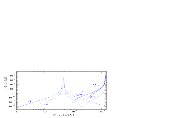
Figure 4: The different annihilation channels evaluated at the freeze out temperature, for a typical choice of parameters, namely, $m_{KK}=3$ TeV, $c_{t_{R}}=-1/2$. “f” denotes all SM fermions except top and bottom.

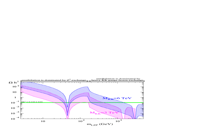
Figure 5: Predictions for $\Omega_{\mbox{\tiny LZP}}\ h^{2}$ for two values of the gauge KK mass $M_{KK}$. Both regions are obtained by varying $g_{10}$ and $c_{\nu_{L}^{\prime}}$. The kink at $m_{LZP}=m_{t}$ corresponds to the opening of the annihilation channel into top quarks.

13 Direct detection

WIMP dark matter can be probed directly via its elastic scattering off nuclei in underground detectors. Several groups are presently carrying out direct searches for galactic halo WIMPs through their elastic scattering off target nuclei. In the absence of positive signal, these experiments set limits on the properties of WIMP dark matter (given some assumptions on halo properties and the local dark matter distribution). Experiments such as CDMS or Edelweiss are now able to probe WIMP-nucleon cross sections of order $10^{-7}$ pb and therefore put constraints on the parameter spaces of various DM candidates. The most stringent constraints come from spin-independent interactions. In particular, any WIMP with a large coupling to the $Z$ gauge boson is severely constrained.

In a significant region of parameter space, our LZP has a large coupling to the Z as detailed in subsections 9.2 and 9.3. Consequently, as is shown in Fig. 7, its entire parameter space should be tested in near future experiments. The elastic scattering cross section is an important quantity as it also controls the rate at which particles accrete into the Earth and the Sun and so determines the signal in the indirect detection experiments as we will see in section 14.

13.1 Elastic scattering cross section

There are actually three potential diagrams contributing to elastic scattering: t-channel $Z$, $Z^{\prime}$ or Higgs exchanges as illustrated in Fig. 6.

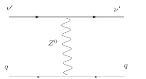
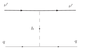
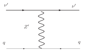
Figure 6: Three diagrams potentially contributing to the elastic scattering cross section between the LZP and a quark. Effectively, only the $Z^{0}$ exchange contributes significantly.

The $Z^{\prime}$ exchange is smaller than the $Z$ exchange since the coupling of light quarks to $Z^{\prime}$ KK modes is small and the mass of $Z^{\prime}$ is at least 3 TeV. Finally, the Higgs-exchange is suppressed by the small ‘Yukawa’ coupling of nucleons. We checked numerically that the last two contributions are indeed negligible. In the following, we will focus on the Z exchange. Note that it leads to a spin-independent (SI) interaction in contrast with supersymmetric dark matter where the Majorana nature of the neutralino makes the $Z$-exchange contribute only in the much less constrained spin-dependent interactions. Given the “weak” but “not so weak” coupling of the LZP to the $Z$, we obtain an elastic scattering cross section for the LZP which is larger than that of the typical LSP in supersymmetry or of the LKP in models with universal extra dimensions [25]. We detail below the calculation.

The 2-body cross section ($1+2\rightarrow 3+4$) may be written as (${\bf p}_{1cm}$ is the momentum of particle 1 in the center of mass frame)

$$\frac{d\sigma}{dq^{2}}=\frac{1}{64\pi s}\frac{1}{|{\bf p}_{1cm}|^{2}}|\langle{\cal M}\rangle|^{2}\ \ \mbox{with}\ \ {p}_{1cm}=\frac{{p}_{1lab}\ m_{2}}{\sqrt{s}}$$ (47)

$|\langle{\cal M}\rangle|^{2}$ is the matrix element squared in a nuclear state, summed over final states and averaged over initial states. Assuming particle 1 is the LZP and particle 2 is the nucleus, we get

$$|{\bf p}_{1cm}|^{2}s={p}_{1lab}^{2}\ m_{2}^{2}=m_{\mbox{\tiny{LZP}}}^{2}v^{2}m_{N}^{2}\ \ \mbox{and}\ \ \frac{d\sigma}{dq^{2}}=\frac{|\langle{\cal M}\rangle|^{2}}{64\pi v^{2}m_{\mbox{\tiny{LZP}}}^{2}m_{N}^{2}}$$ (48)

The elastic scattering cross section at zero momentum transfer, $\sigma_{0}$, is defined as

$$\frac{d\sigma}{dq^{2}}\equiv\frac{\sigma_{0}}{4\mu^{2}v^{2}}F^{2}(q^{2})\ \ \ \ \ \ \ \mbox{where}\ \ F^{2}(q^{2}=0)=1\ \ \ \ \ \ \mbox{and}\ \ \mu=\frac{m_{\mbox{\tiny{LZP}}}m_{N}}{m_{\mbox{\tiny{LZP}}}+m_{N}}$$ (49)

$F^{2}(q^{2})$ is the nuclear form factor and $\mu$ the reduced mass. Thus,

$$\sigma_{0}\equiv\frac{|{\cal\langle M\rangle}|^{2}_{q^{2}=0}}{16\pi(m_{\mbox{\tiny{LZP}}}+m_{N})^{2}}$$ (50)

In the calculation of $|{\cal\langle M\rangle}|^{2}$, we only keep the dominant contribution due to t-channel $Z$ exchange. In the non-relativistic limit, $q^{2}\ll m_{Z}^{2}$, the corresponding effective lagrangian at the quark level reads:

$$\frac{g_{Z}^{\nu^{\prime}_{R}}}{4m_{Z}^{2}}\ \left[\overline{u}_{\mbox{\tiny{LZP}}}\gamma^{\mu}u_{\mbox{\tiny{LZP}}}+\overline{u}_{\mbox{\tiny{LZP}}}\gamma^{\mu}\gamma^{5}u_{\mbox{\tiny{LZP}}}\right]\times\left[(g^{q}_{L}+g^{q}_{R})\overline{u}_{q}\gamma_{\mu}u_{q}+(g^{q}_{R}-g^{q}_{L})\overline{u}_{q}\gamma_{\mu}\gamma^{5}u_{q}\right]$$ (51)

where

$$g_{L}^{u}=\frac{(\frac{1}{2}-\frac{2}{3}\sin^{2}\theta_{W})e}{\sin\theta_{W}\cos\theta_{W}}\ \ \ \ \ g_{R}^{u}=\frac{(-\frac{2}{3}\sin^{2}\theta_{W})e}{\sin\theta_{W}\cos\theta_{W}}\ \ \ \ g_{L}^{d}=\frac{(-\frac{1}{2}+\frac{1}{3}\sin^{2}\theta_{W})e}{\sin\theta_{W}\cos\theta_{W}}\ \ \ \ \ g_{R}^{d}=\frac{(\frac{1}{3}\sin^{2}\theta_{W})e}{\sin\theta_{W}\cos\theta_{W}}$$

The next step is to evaluate matrix elements in a nucleon state. Given the fact that $\langle\overline{u}_{q}\gamma^{i}u_{q}\rangle\approx 0$ and $\langle\overline{u}_{q}\gamma^{0}\gamma^{5}u_{q}\rangle\approx 0$, the effective four-fermion interaction reduces to :

$$\frac{g_{Z}^{\nu^{\prime}_{R}}}{4m_{Z}^{2}}\ \left(\left[\overline{u}_{\mbox{\tiny{LZP}}}\gamma^{0}u_{\mbox{\tiny{LZP}}}\right]\left[(g^{q}_{L}+g^{q}_{R})\overline{u}_{q}\gamma_{0}u_{q}\right]+\left[\overline{u}_{\mbox{\tiny{LZP}}}\gamma^{i}\gamma^{5}u_{\mbox{\tiny{LZP}}}\right]\left[(g^{q}_{R}-g^{q}_{L})\overline{u}_{q}\gamma_{i}\gamma^{5}u_{q}\right]\right)$$ (52)

The first term will contain the operator $\langle\overline{u}_{q}\gamma_{0}u_{q}\rangle=\langle u^{\dagger}_{q}u_{q}\rangle$ which simply counts valence quarks in the nucleon. This part of the vector interaction is coherent. We then sum over nucleons in the nucleus. The second term leads to a spin-dependent (SD) interaction. We obtain:

$$|\langle{\cal M}\rangle|^{2}_{SI}=\frac{8\ m_{\mbox{\tiny{LZP}}}^{2}\times 4\ m_{N}^{2}S_{\mbox{\tiny SI}}(q)\ 4\pi\times b_{N}^{2}}{2\ (2J+1)}$$ (53)

$$|\langle{\cal M}\rangle|^{2}_{SD}=\frac{4\ m_{\mbox{\tiny{LZP}}}^{2}\times 4\ m_{N}^{2}S_{\mbox{\tiny SD}}(q)\ 8\pi}{2\ (2J+1)}$$ (54)

$$b_{N}=Zb_{p}+(A-Z)b_{n}\ \ ,\ \ b_{p}=\frac{g_{Z}^{\nu^{\prime}_{R}}\ e\ (1-4\sin\theta_{W})}{8M_{Z}^{2}\sin\theta_{W}\cos\theta_{W}}\ \ \ \mbox{and}\ \ \ b_{n}=-\frac{g_{Z}^{\nu^{\prime}_{R}}\ e}{8M_{Z}^{2}\sin\theta_{W}\cos\theta_{W}}$$ (55)

$S_{\mbox{\tiny SI}}(q)$ and $S_{\mbox{\tiny SD}}(q)$ are the nuclear form factors defined as $S_{\mbox{\tiny SI}}(q)=(2J+1)F^{2}(q)/(4\pi)$ and $S_{\mbox{\tiny SD}}(q)=(2J+1)\Lambda^{2}J(J+1)F^{2}(q)/\pi$ [35]. The coefficient $\Lambda$ depends on the spin $J$ of the nucleus, $\langle S_{p}\rangle$ and $\langle S_{n}\rangle$ the parts of the nucleus’ spin carried by protons and neutrons.

$$\Lambda=\frac{a_{p}\langle S_{p}\rangle+a_{n}\langle S_{n}\rangle}{J}\ \ \ ,\ \ \ a_{p,n}=\sum_{u,d,s}b^{\prime}_{q}\Delta^{(p,n)}q\ \ \ ,\ \ \ b^{\prime}_{q}=\frac{g_{Z}^{\nu^{\prime}_{R}}(g_{R}^{q}-g_{L}^{q})}{4M_{Z}^{2}}$$ (56)

As a result:

$$\sigma_{0}^{SI}=\frac{\mu^{2}b_{N}^{2}}{\pi}=\frac{\left(g_{Z}^{\nu^{\prime}_{R}}\right)^{2}\mu^{2}e^{2}}{64\pi m_{Z}^{4}\sin^{2}\theta_{w}\cos^{2}\theta_{w}}\left[Z(1-4\sin^{2}\theta_{w})-(A-Z)\right]^{2}$$ (57)

$$\sigma_{0}^{SD}=\frac{4\mu^{2}\Lambda^{2}J(J+1)}{\pi}$$ (58)

From now, given the fact that experiments are carried on heavy nuclei such as germanium for instance, we will ignore the SD contribution which is smaller than the SI one by a factor $1/(A-Z)^{2}$.

13.2 WIMP-nucleon cross section

The SI cross-section data is commonly normalised to a single nucleon to compare results from different experiments (which use different target nuclei). For sufficiently low momentum transfer, and assuming that the WIMP has the same interaction for protons and neutrons, the $A$ scattering amplitudes add up to give a coherent cross section $\propto A^{2}$. Therefore, experimentalists express their bound in terms of the WIMP-nucleon cross sections, using this $A^{2}$ scaling. We follow this convention in our Fig. 7. However, the WIMP has typically diffferent interactions between protons and neutrons and the experimental bound has to be interpreted with a bit of care. This is the case of Dirac neutrinos (like our LZP), where the interactions to protons is suppressed by $(1-4\sin^{2}\theta_{W})^{2}$ and the interaction is essentially due to neutrons. So, in order to obtain the WIMP-nucleon cross section, one should rather use the scaling $(A-Z)^{2}$. To interpret data, one should also keep in mind that experimental limits use the prevailing convention of assuming that the local halo density of dark matter is 0.3 GeV/cm³, and that the characteristic halo velocity $v_{0}$, is 220 km s^-1 and the mean earth velocity $v_{E}$ is 232 km s^-1. Some uncertainties are associated with these numbers.

The nucleon-WIMP cross section is defined as

$$\sigma_{p,n}=\sigma_{0}\frac{\mu_{p,n}^{2}}{\mu^{2}_{A}}\frac{C_{p,n}}{C_{A}}\ \ ,\ \ \mu_{A}=\frac{m_{\chi}m_{A}}{m_{\chi}+m_{A}}\ \ ,\ \ \sigma_{0}\propto\mu^{2}_{A}C_{A}$$ (59)

$$\mu_{p,n}=\frac{m_{\chi}m_{p,n}}{m_{\chi}+m_{p,n}}\approx m_{p,n}$$ (60)

For a scalar interaction involving a $Z$ exchange, $C_{A}=(Z(1-4\sin^{2}\theta_{W})-(A-Z))^{2}$. Then, using $\sin^{2}\theta_{W}=0.23120$

$$C_{p}=(1-4\sin^{2}\theta_{W})=0.0752\ll 1\ \mbox{and}\ C_{n}=1$$ (61)

which leads to

$$\sigma_{n}=\sigma_{0}\frac{m_{p}^{2}}{\mu^{2}}\frac{(1-4\sin^{2}\theta_{W})^{2}}{(Z(1-4\sin^{2}\theta_{W})-(A-Z))^{2}}$$ (62)

$$\sigma_{p}=\sigma_{0}\frac{m_{p}^{2}}{\mu^{2}}\frac{(1-4\sin^{2}\theta_{W})^{2}}{(Z(1-4\sin^{2}\theta_{W})-(A-Z))^{2}}\approx 5.65\times 10^{-3}\sigma_{n}$$ (63)

As can be seen in Fig. 7, the LZP-nucleon cross section is large ($\gtrsim 10^{-10}$ pb) so that our models will be tested in the near future.

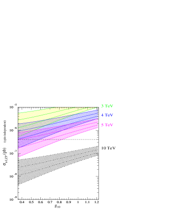
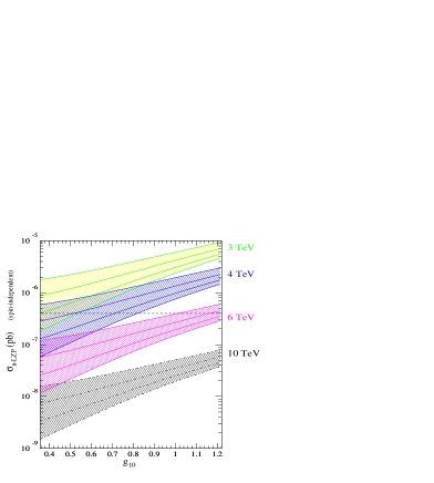
Figure 7: Predictions for $\sigma_{n,LZP}$. The left plot has been derived assuming that the Higgs is localized exactly on the TeV brane and for $m_{KK}=$3, 4, 5, 10 TeV. The right plot corresponds to the case where the Higgs is the fifth component of a gauge boson (i.e., a PGB) with a profile in the bulk given by Eq. (101). Those two cases lead to significantly different LZP–Z couplings. Indeed, both the Yukawa coupling of the Higgs to $\nu^{\prime}_{L}$ and $\nu^{\prime}_{R}$ and the $Z-Z^{\prime}$ mixings are modified by the profile (see sections 9.2 and 9.3). We see that the precise value of the LZP–Z coupling (which will vary from one model of EW symmetry breaking to another) is crucial for event rates at direct detection experiments. At least, models with the Higgs localized on the TeV brane are quite constrained here. The horizontal line indicates the experimental limit [36] which only applies to a range of WIMP masses.

14 Indirect detection

Indirect dark matter searches consist in looking for products of dark matter annihilation including gamma-rays, positrons, anti-protons and neutrinos. Such signal would come from regions where the dark matter density is large, like in the center of the galaxy. One difficulty is that the expected flux depends very sensitively on the dark matter profile at the galactic center, something which is still poorly known. We also expect that WIMPs annihilate in the Sun and the Earth, in which case, uncertainties in their distribution are much more under control. We focus on this signal in the following.

When equilibrium is reached between the rate $C^{\odot}$ at which WIMPs are captured in the Sun (determined by the WIMP-nucleus elastic scattering cross section) and the annihilation rate $A^{\odot}$, the annihilation rate in the Sun is maximized and given by [37]

$$\Gamma=\frac{1}{2}\,C^{\odot}\,\tanh^{2}\left(\sqrt{C^{\odot}A^{\odot}}\,t_{\odot}\right)\;$$ (64)

where $t_{\odot}\simeq 4.5$ billion years. The equilibrium condition is $\sqrt{C^{\odot}A^{\odot}}t_{\odot}\gg 1$. $A^{\odot}$ is given by

$$A^{\odot}=\frac{\langle\sigma v\rangle}{V_{eff}}\ \ \ \ \mbox{where}\ \ V_{eff}=5.7\times 10^{27}\mbox{cm}^{3}\left(\frac{100\mbox{GeV}}{m_{WIMP}}\right)^{3/2}$$ (65)

Since we have a large elastic scattering cross section (much larger than the LSP in SUSY and LKP in UED) we anticipate interesting signals. However, remember that the Sun is mainly made of protons and scattering of the LZP with protons is suppressed. Fortunately, interactions with helium should provide observable signal. The capture rates for spin-dependent and spin-independent interactions are given by [37]

$$C_{\mathrm{SD}}^{\odot}\simeq 3.35\times 10^{20}\,\mathrm{s}^{-1}\left(\frac{\rho_{\mathrm{local}}}{0.3\,\mathrm{GeV}/\mathrm{cm}^{3}}\right)\left(\frac{270\,\mathrm{km/s}}{\bar{v}_{\mathrm{local}}}\right)^{3}\left(\frac{\sigma_{\mathrm{H,SD}}}{10^{-6}\,\mathrm{pb}}\right)\left(\frac{100\,\mathrm{GeV}}{m_{\rm{LZP}}}\right)^{2}$$ (66)

$$C_{\mathrm{SI}}^{\odot}\simeq 1.24\times 10^{20}\,\mathrm{s}^{-1}\left(\frac{\rho_{\mathrm{local}}}{0.3\,\mathrm{GeV}/\mathrm{cm}^{3}}\right)\left(\frac{270\,\mathrm{km/s}}{\bar{v}_{\mathrm{local}}}\right)^{3}\left(\frac{2.6\,\sigma_{\mathrm{H,SI}}+0.175\,\sigma_{\mathrm{He,SI}}}{10^{-6}\,\mathrm{pb}}\right)\left(\frac{100\,\mathrm{GeV}}{m_{\rm{LZP}}}\right)^{2}$$ (67)

$\rho_{\mathrm{local}}$ is the local DM density. $\bar{v}_{\mathrm{local}}$ is the local rms velocity of halo DM particles. $\sigma_{\mathrm{H,SD}}$ and $\sigma_{\mathrm{H,SI}}$ are the spin-dependent and spin-independent, LZP-on-proton (hydrogen) elastic scattering cross sections, $\sigma_{\mathrm{He,SI}}$ is the spin-independent, LZP-on-helium elastic scattering cross section. The SI cross sections are trivially obtained from Eq. 57:

$$\sigma_{H,SI}=\frac{\left(g_{Z}^{\nu^{\prime}_{R}}\right)^{2}e^{2}\mu^{2}_{H}(1-4\sin^{2}\theta)^{2}}{64\pi M_{Z}^{4}\sin^{2}\theta\cos^{2}\theta}\ \ \ ,\ \ \ \sigma_{He,SI}=\frac{\left(g_{Z}^{\nu^{\prime}_{R}}\right)^{2}e^{2}\mu^{2}_{He}\left(2(1-4\sin^{2}\theta)-2\right)^{2}}{64\pi M_{Z}^{4}\sin^{2}\theta\cos^{2}\theta}$$ (68)

where $\mu_{H,He}=m_{\mbox{\tiny LZP}}m_{H,He}/(m_{\mbox{\tiny LZP}}+m_{H,He})$. It is clear that $\sigma_{He,SI}$ dominates by a factor $10^{4}$. The SD interaction (see Eq. 58) is given by

$$\sigma_{H,SD}=\frac{3\ \mu^{2}_{H}\Lambda^{2}}{\pi}\ \ \ ,\ \ \ \Lambda=a_{p}\ \ \ ,\ \ \ a_{p}=\frac{e\ g_{Z}^{\nu^{\prime}_{R}}}{8M_{Z}^{2}\cos\theta\sin\theta}\left[-\Delta u+\Delta d+\Delta s\right]$$ (69)

where $\Delta u=0.78\pm 0.02$, $\Delta d=-0.48\pm 0.02$ and $\Delta s=-0.15\pm 0.02$ [38] are the spins carried by the quarks u, d, s respectively in the proton. In fig. 8, we have plotted $\sigma_{He,SI}$, $\sigma_{H,SD}$. In fig. 9, we plotted $\sqrt{C^{\odot}A^{\odot}}t_{\odot}$ evaluated at $\langle\sigma_{anni}\ v\rangle\approx 1$ pb, the value of the annihilation cross section leading to the correct relic density. This shows that throughout the parameter region leading to the ideal relic density, the Sun always reaches equilibrium between the LZP capture and annihilation. The event rate and prospects for indirect detection will be provided elsewhere [39].

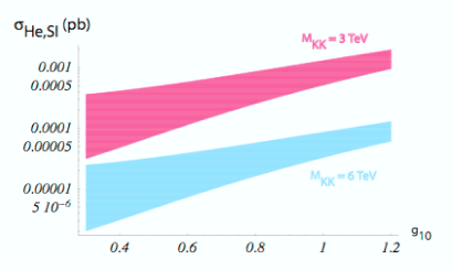
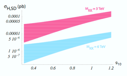
Figure 8: Values of $\sigma_{He,SI}$ $\sigma_{H,SD}$ for $m_{KK}=3$ TeV (red) and $m_{KK}=6$ TeV (blue). Each region is obtained by varying $c_{\nu^{\prime}_{L}}$ in the range $[c_{t_{R}}-0.5,c_{t_{R}}+0.5]$.

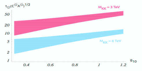
Figure 9: $\sqrt{C^{\odot}A^{\odot}}t_{\odot}$ evaluated at $\langle\sigma_{anni}\ v\rangle=1$ pb. We see that it is always larger than 1, meaning that equilibrium between capture and annihilation is reached in the Sun.

15 Collider phenomenology

A very exciting aspect of these models is the potential for discovery of KK modes at colliders. This is to be contrasted with previous studies carried out in Randall-Sundrum background, where the emphasis has been on $(++)$ type of boundary conditions, in which case it might be difficult to produce KK modes at the LHC since the KK masses have to be larger than 3 TeV. In our $SO(10)$ model, as we already emphasized in section 4, all KK modes in the multiplet with $t_{R}^{(0)}$ (except KK modes for $t_{R}$ itself) are expected to be light because they have ($-+$) BC as well as $c$ close to $-1/2$. Since the splittings in $c$ are unknown, we will take these masses to be free parameters. Another interesting aspect is that most of the $Z_{3}$-charged fermions from the $t_{R}$ multiplet cannot decay very easily. The reason is that they have to eventually decay into the LZP (and SM particles, i.e., zero-modes) and, in this multiplet, only $t_{R}$ has zero mode. As a result, these decays have to go through a certain number of virtual states. This leads to very distinctive signatures which we will present in this section.

We repeat that KK modes of ($-+$) gauge bosons might be too heavy to be significantly produced at the LHC ($M_{KK}\gtrsim 3$ TeV). Similarly, ($-+$) KK fermions coming from other multiplets (with $c\gtrsim 0$) and ($++$) KK fermions are considered too heavy. For instance, $t_{R}^{(1)}$ in the multiplet we are interested in is heavy. Actually, a detailed calculation would be required to determine whether the strong coupling of heavy KK modes can compensate for the large mass suppression in the production cross-section. In contrast, colored light KK modes from $t_{R}$ multiplet (with a mass $\lesssim 1$ TeV) will be copiously produced at the LHC.

Before discussing collider signatures, let us mention that we do not expect any experimental constraint coming from the additional $U(1)_{B}$ gauge boson. As said earlier, we couple it to a Planckian vev on the UV brane. This mimics $(-+)$ BC to a good approximation. The coupling of light fermions to KK modes of $U(1)_{B}$ is negligible compared to the $4D$ would-be’ zero-mode $U(1)_{B}$ gauge coupling since light fermions are localized near the Planck brane where $U(1)_{B}$ KK modes effectively vanish. Whereas, the coupling of $t_{R}$ to $U(1)_{B}$ KK modes is enhanced by $\sqrt{k\pi r_{c}}$ compared to $4D$ gauge coupling since both $t_{R}$ zero-mode and $U(1)_{B}$ KK modes are localized near the TeV brane. Also, the $U(1)_{B}$ KK modes do not mix with zero-mode of $Z$ (unlike $Z^{\prime}$ KK modes) since the Higgs does not carry $B$. Thus, we see that KK masses of $\sim$ few TeV for $U(1)_{B}$ gauge boson are not constrained by current data.

It is clear that in the absence of GUT bulk breaking, $SU(2)_{L}$-charged KK modes in the $t_{R}$ multiplet such as $b_{L}^{\prime}$, $t_{L}^{\prime}$, $\nu_{\tau,L}^{\prime}$ and $\tau_{L}^{\prime}$ decay very slowly (see section 7.3). Thus, they will cross the detector and those which carry an electric charge will easily be detected due to their CHAMP (stable charged massive particles)-like signatures. Colored particles hadronize and what is detected is some charged KK meson made of a light quark and a KK $b_{L}^{\prime}$ or $t_{L}^{\prime}$. In the presence of GUT bulk breaking of the unified gauge symmetry, $SU(2)_{L}$-charged KK modes can decay due to $X^{\prime}-X_{S}$ mixing (see Fig. 12). The size of this mixing will depend on the profile of the GUT breaking scalar $\Sigma$ in the bulk. If this mixing is too small then decay will take place outside the detector. On the other hand, if $\Sigma$ has a flat profile, the mixing is large and the decay easily takes place in the detector, although the lifetime is quite sensitive to the mass splitting (as shown in section 7.4). This situation leads to very interesting signatures.

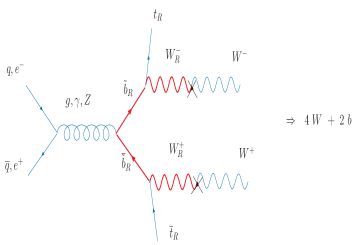
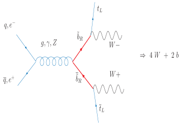
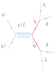
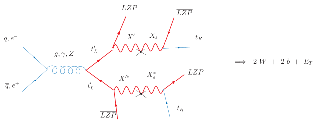
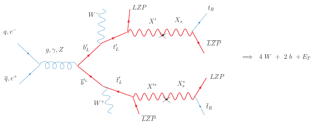
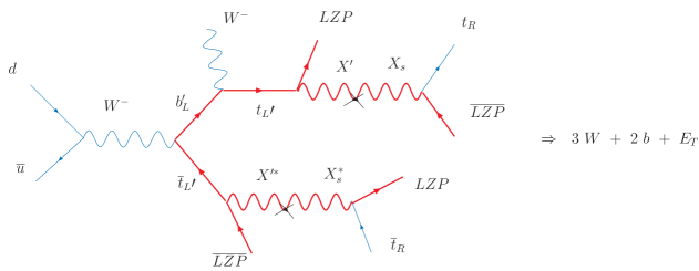
Figure 10: Production of KK quarks

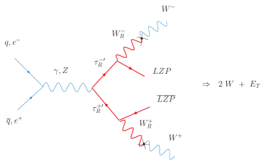
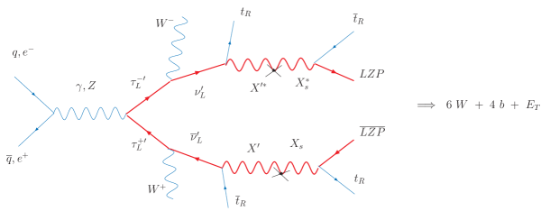
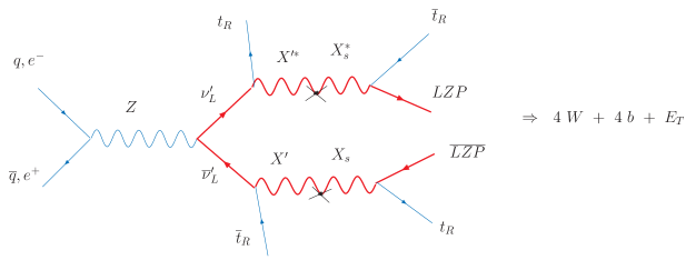
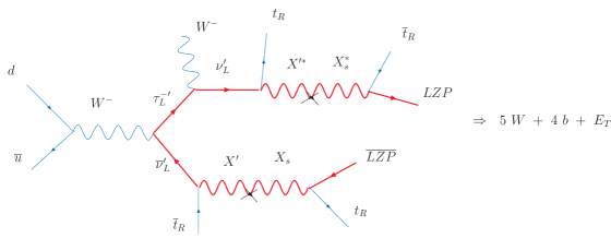
Figure 11: Production of KK leptons. $\nu^{\prime}_{L}$ refers to $\nu^{\prime}_{\tau,L}$.

We now list all the decays which are illustrated in Fig.10 and 11:

$$\tilde{b}_{R}\rightarrow b_{L}H,\;t_{L}W_{long.}$$

$$\tilde{b}_{R}\rightarrow t_{R}\,W^{-}\ \ \ \mbox{via}\ W_{R}\mbox{-}W_{L}\ \ \mbox{mixing}$$

$$t^{\prime}_{L}\rightarrow t_{R}\,\nu_{R}^{\prime}\,\overline{\nu}_{R}^{\prime}\ \ \ \mbox{via}\ X^{\prime}\mbox{-}X_{s}\ \ \mbox{mixing}$$

$$b^{\prime}_{L}\rightarrow t_{R}\,\nu_{R}^{\prime}\,\overline{\nu}_{R}^{\prime}\,W^{-}\ \ \ \mbox{via}\ X^{\prime}\mbox{-}X_{s}\ \ \mbox{mixing}$$

$$\tau^{\prime-}_{R}\rightarrow\nu^{\prime}_{R}\,W^{-}\ \ \ \mbox{via}\ W_{R}\mbox{-}W_{L}\ \ \mbox{mixing}$$

$$\tau^{\prime-}_{L}\rightarrow\nu^{\prime}_{R}\,t_{R}\,\overline{t}_{R}\,W^{-}\ \ \ \mbox{via}\ X^{\prime}\mbox{-}X_{s}\ \ \mbox{mixing}$$

$$\nu^{\prime}_{\tau,L}\rightarrow\nu^{\prime}_{R}\,t_{R}\,\overline{t}_{R}\ \ \ \mbox{via}\ X^{\prime}\mbox{-}X_{s}\ \ \mbox{mixing}$$

The effective couplings of $t_{L}^{\prime}$ to $\nu_{R}^{\prime}$ and $\nu_{L}^{\prime}$ to $t_{R}$ due to $X^{\prime}-X_{s}$ mixing are

$$g_{\nu^{\prime}_{R},t_{L}^{\prime},X_{s}} = \frac{g_{10}}{\sqrt{2}}\sqrt{k\pi r_{c}}\times{\cal F}_{\nu^{\prime}_{R},t_{L}^{\prime}}\times P_{R}\times{\cal M}_{X^{\prime}-X_{s}}$$ (70)

$$g_{\nu^{\prime}_{\tau,L},t_{R},X_{s}} = g_{\nu^{\prime}_{R},t_{L}^{\prime},X_{s}}\times\frac{{\cal F}_{\nu^{\prime}_{\tau,L},t_{R}}}{{\cal F}_{\nu^{\prime}_{R},t_{L}^{\prime}}}$$ (71)

$${\cal M}_{X^{\prime}-X_{s}} \sim \frac{M_{GUT}^{2}}{M_{KK}^{2}}\,k\lambda_{5}\frac{v}{\Lambda}$$ (72)

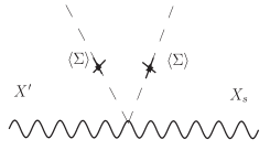
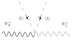
Figure 12: Diagrams leading to $X^{\prime}-Xs$ and $W_{R}^{\pm}-W_{L}^{\pm}$ mixings.

The ${\cal F}\sim 1$ are the form factors reflecting the overlap between the wave functions. $P_{R}$ is the projector to remind that we focus on only one chirality, i.e., $(-+)$ of the LZP (the other chirality is localized near the Planck brane and its coupling to $X_{s}$ is suppressed). ${\cal M}_{X^{\prime}-X_{s}}$ is the mixing factor due to the GUT breaking vev of the bulk scalar field $\Sigma$. $M_{GUT}/M_{KK}\lesssim 1/5$ is a measure of bulk GUT breaking. $k\lambda_{5}\sim{\cal O}(1)$, $v$ is the Higgs vev and $\Lambda\sim$ 10 TeV is the cut off on the IR brane.

The coupling of $\tilde{b}_{R}$ to the Higgs and $(t,b)_{L}$ is $\lambda_{t\;4D}f\left(c_{R}\right)$ (see section 7.1). The effective couplings of $\tau^{\prime-}_{R}$ to $W^{-}$ and $\tilde{b}_{R}$ to $W^{-}$ due to $W_{R}-W_{L}$ mixing resulting from EW symmetry breaking are:

$$g_{\nu^{\prime}_{R},\tau_{R}^{\prime-},W^{-}} = \frac{g_{10}}{\sqrt{2}}\sqrt{k\pi r_{c}}\times{\cal F}_{\nu^{\prime}_{R},\tau_{R}^{\prime}}\times P_{R}\times{\cal M}_{W_{R}-W_{L}}$$ (73)

$$g_{\tilde{b}_{R},t_{R},W^{-}} = g_{\nu^{\prime}_{R},\tau^{\prime-}_{R},W^{-}}\times\frac{{\cal F}_{\tilde{b}_{R},t_{R}}}{{\cal F}_{\nu^{\prime}_{R},\tau^{\prime-}_{R}}}$$ (74)

$${\cal M}_{W_{R}-W_{L}} = \frac{g_{10}}{g}\sqrt{2k\pi r_{c}}\frac{M_{W}^{2}}{M_{KK}^{2}}$$ (75)

Again, the projector expresses the fact that only one chirality of the LZP has a non-suppressed coupling to $W_{R}$. Note that, in contrast, the direct interactions of our $(-+)$ KK fermions to zero-mode gauge bosons, as shown in the production process in the figures, are vector-like. This is because zero-mode gauge bosons have a flat profile (unlike KK modes) and couple identically to both chiralities of KK fermions.

16 Baryogenesis

16.1 Relating dark matter to the baryon asymmetry

Since our colorless dark matter particle carries baryon number, it is very tempting to investigate whether the origin of the apparent matter-antimatter asymmetry of the universe is that antimatter is stored in dark matter. In other words, in a universe where baryon number is a good symmetry, the negative baryonic charge would be carried by DM, while the equal and opposite baryonic charge would be carried by ordinary SM quarks. This would provide a beautiful common explanation for these two major cosmological puzzles.

Imagine that an asymmetry between $\nu^{\prime}_{R}$ and $\overline{\nu^{\prime}}_{R}$ is created due to the CP-violating out of equilibrium decay of KK gauge boson $X^{\prime}$: $X^{\prime}$ does not carry baryon number but decays into the LZP and an anti-top quark. The resulting asymmetry between the LZP and $\overline{LZP}$ (chosen to be negative) is equal to the asymmetry between the quark and antiquark. Consequently, dark matter would store the overall negative baryonic charge which is missing in the visible quark sector. The calculation of the relic density of dark matter is now quite different. It does not depend directly on the calculation of the annihilation cross section of the LZP but rather on the abundance of $X^{\prime}$ at the time of its decay. Indeed, in the out-of equilibrium decay scenario, $Y_{asym}\sim\epsilon\ Y_{X^{\prime}}/g_{*}$ where $Y_{asym}$ is $(\overline{n}_{LZP}-{n}_{LZP})/s$, $Y_{X^{\prime}}=n_{X^{\prime}}/s$ is the relic abundance $X^{\prime}$ would have today if it had not decayed, $s$ is the entropy density, $g_{*}$ is the number of relativistic degrees of freedom at the time of the decay and $\epsilon$ denotes CP-violation in the decay of $X^{\prime}$.

It is well-known that to explain the baryon asymmetry of the universe from an out of equilibrium decay, it is necessary that the decaying particle be overabundant. That is for instance what is required in leptogenesis where one needs the RH neutrino to be out of thermal equilibrium so that its number density can be large. The problem with the $X^{\prime}$ particle is that it has large gauge interactions and therefore large annihilation cross sections (via the s-channel gluon exchange) and, if we assume that it was at thermal equilibrium initially, then it will not be overabundant after freeze-out.

Remember that $X^{\prime}$ would freeze out at a temperature $T_{F}\sim m_{X^{\prime}}/x_{F}$ where $x_{F}\sim 25$ so for $m_{X^{\prime}}\gtrsim$3 TeV, $T_{F}\gtrsim 120$ GeV. Then, the only situation we can consider is that the reheat temperature of the universe is below the “would-be” freeze-out temperature of $X^{\prime}$ and assume that $X^{\prime}$ is produced non thermally and abundantly at the end of inflation. The thermal history is poorly known in RS1 geometries [41] and we are unable at this point to make any more precise statement. However, assuming that $X^{\prime}$ is indeed overabundant, there is a potentially interesting mechanism for relating dark matter and the baryon asymmetry as follows.

Baryon number conservation leads to $\frac{1}{3}(n_{\mbox{\tiny LZP}}-\overline{n}_{\mbox{\tiny LZP}})=\overline{n}_{b}-n_{b}$. Therefore,

$$\frac{1}{3}\ Y_{asym}\approx\frac{{n}_{b}}{s}\sim 10^{-10}$$ (76)

where in the last step we have assumed that annihilation of baryons with antibaryons after the production of the asymmetry is efficient enough so that the left over $\overline{n}_{b}$ are negligible compared to the excess of baryons. What we have to ensure is that $X^{\prime}$ decays out of equilibrium, but before the baryons stop annihilating so that the relic density of baryons is indeed given by the asymmetry. $X^{\prime}$ can decay because of the mixing with $X_{s}$ (see Fig. 12) and the size of this mixing depends on the size and profile along the extra dimension of the vev of the scalar $\Sigma$ which breaks $SO(10)$ in the bulk. Thus, it is possible that the above condition on the decay of $X^{\prime}$ is satisfied.

If the LZP and anti-LZP can annihilate sufficiently after the $X^{\prime}$-decay, then the only dark matter left is given by the asymmetry, i.e., $Y_{DM}=Y_{asym}$. Clearly, we need a large LZP annihilation cross section for this to happen. This will occur when the LZP annihilation takes place near the resonances (see Figs. 4 and 5). In the case that only the excess of anti-LZPs remain, since $\rho_{\mbox{\tiny DM}}\approx 6\ \rho_{b}$ and $\rho_{\mbox{\tiny DM}}=m_{\mbox{\tiny LZP}}Y_{asym}s=3m_{\mbox{\tiny LZP}}{Y_{b}}s$, we obtain that

$$m_{\mbox{\tiny LZP}}\approx 2\ \mbox{GeV}.$$ (77)

This mass is not near a resonance so that, within our strict framework, we cannot guarantee that DM is just given by the LZP asymmetry. Increasing the LZP-$Z$ coupling is a way to increase the annihilation cross section. Note that such a low mass is not constrained at all by direct detection experiments. However, there are constraints from the $Z$ width. It is quite clear from Fig. 5 that even for the largest allowed LZP-Z coupling, the relic density of a 2 GeV LZP is still too large by two orders of magnitude.

So, one has to modify the model in such a way to increase the annihilation cross section at LZP masses $\approx 2$ GeV. There could be additional annihilation channels playing a role even for small LZP masses. It might be possible to open the annihilation channel via the Higgs exchange. An alternative would be to assume that the reheat temperature is quite low $\lesssim{\cal O}$(1 GeV) so that the LZP never reaches thermal equilibrium and its initial abundance is suppressed. This solves the problem of overclosure of the universe by LZPs. We still have to guarantee a large enough annihilation cross section of the LZP for the validity of Eq. 77.

Away from the regions where the annihilation cross section is large ($>$ 1 pb), we can neglect the effect of the asymmetry on the relic density of dark matter and the relation between $\Omega_{DM}$ and $\Omega_{b}$ is less straightforward.

Note that we did not consider the decay of $X_{s}$ because it has too large couplings to $t_{R}$ and the LZP so that it would not decay out of equilibrium.

Finally, because of $Z_{3}$ conservation, the LZP cannot annihilate with itself into a SM final state (it can annihilate only with the anti-LZP). Thus, there is no annihilation diagram of the simple form LZP LZP $\rightarrow A+B$ where $A$ and $B$ are SM particles leading to the transfer of baryon number from the dark sector to the visible sector (hence washout of the baryon asymmetry). Processes such as LZP LZP $\rightarrow$ anti-LZP $+$ SM are allowed by the $Z_{3}$ symmetry: a detailed study would be required to see if they can lead to significant washout of the baryon asymmetry or not.

16.2 GUT baryogenesis at the TeV scale

We now turn to a very different idea. In this paper, we mainly talked about the model with gauged baryon number. However, we stressed in subsection 6.2 the fact that proton stability can be guaranteed by assuming lepton number symmetry instead of baryon number. This is actually an economical solution since it also forbids dangerous lepton number violation due to Majorana masses on the TeV brane. Unfortunately, there is no DM particle in this case. An intriguing feature of this model though is the possibility to observe baryon number violation at colliders, for instance via the production of (perhaps off-shell) KK $X$ gauge boson which then decays into $u$ and $d$ quarks, violating $B$.

We now want to expose some potentially interesting baryogenesis idea, even if at first sight it seems difficult to achieve in our particular framework. In traditional GUT baryogenesis, one uses the out of equilibrium $B$-violating decay of GUT scale mass $X/Y$ gauge bosons. However, if the $X/Y$ gauge bosons have a mass at the TeV scale, for their decay to be out-of equilibrium, the gauge coupling has to be smaller than about $10^{-8}$. This comes from equating the decay rate to the expansion rate: $g^{2}M_{X}/(8\pi)\sim T^{2}/M_{Pl}$. In our model, the decays which violate $B$ (without violating $L$) are $X^{\prime}\rightarrow dd$, $Y^{\prime}\rightarrow ud$ and $X\rightarrow uu$.

As mentioned in section 8.4, quarks of the third generation originate in different multiplets to account for their different $c$’s. Whereas, quarks of the 1st and 2nd generations can come from the same multiplet. So, $X$-type gauge bosons can decay into two quarks from the 1st or 2nd generation only. However, even though the 1st and 2nd generation quarks are localized near the Planck brane (while the $X$-type gauge bosons are near the TeV brane), their coupling to $X$-type gauge boson is typically $g\sim 10^{-5}$ for 1st generation (and larger for 2nd generation) to be compatible with their Yukawa couplings. Thus, it is likely that the decays will not be out of equilibrium.

In any case, assuming some mechanism to further suppress the couplings of $X$-type gauge bosons, one would also have to check that the new CP violating sources required for baryogenesis in the X/Y sector are not in conflict with current experimental constraints. And again, we would need a reheat temperature below, say, $120$ GeV to insure that $X,Y$ can be overabundant when they decay.

17 Conclusion

In this paper, we have studied the issue of baryon-number violation in a GUT in a non supersymmetric warped extra dimension. One way to suppress proton decay is to impose gauged baryon-number symmetry. We showed how this solution to the proton stability problem leads to a stable KK particle, the stability being guaranteed by a combination of baryon-number and color, named $Z_{3}$. $Z_{3}$ is already present in the Standard Model at the renormalizable level, though SM particles are not charged under it. This is similar to $R$-parity leading to a stable particle in SUSY models.

Our firm prediction is that the lightest $Z_{3}$-charged particle (LZP) is a GUT partner of the top quark and that its lightness is related to the top quark’s heaviness. At this stage, we are not able to predict which particle in the top multiplet is the LZP, but as far as dark matter is concerned, the LZP must have gauge quantum numbers of a RH neutrino. We can ensure that this is the case due to the breaking of the GUT in the bulk. We showed in detail how this exotic RH neutrino acts as a WIMP and why its relic density is of the right value for masses in the 10 GeV – a few TeV range. We also explained why the entire parameter space of this DM candidate will be tested at near future direct detection experiments.

The breaking of the GUT has direct observable effects at the TeV scale. The other KK modes in the top quark multiplet are also light. Because of their strong (QCD) coupling, the quark-like states can easily be produced at colliders and be detected via their distinctive decay into the LZP. The production of these other exotic, light partners of the top quark at high-energy colliders is an interesting manifestation of unification in AdS.

We studied both models with the Higgs localized on the TeV brane and with a profile for the Higgs in the bulk (but still localized near the TeV brane). Our qualitative results apply to any warped extra-dimensional GUT with electroweak symmetry breaking localized near the TeV brane. For example, our models can be seen as a GUT embedding of the recently studied Higgsless models in warped space [16]. The choice of Pati-Salam or $SO(10)$ gauge group over $SU(5)$ is dictated by the need to incorporate custodial isospin symmetry, $SU(2)_{R}$, to satisfy electroweak precision constraints. Actually, up to factors of $O(1)$, we expect that our quantitative results also apply to Higgsless models. Of course, in these models, the KK scale is no longer a free parameter since it is related to the $W$ and $Z$ masses.

There are many issues one could investigate further. It would be interesting to consider variations of the model we presented. For instance, as far as bulk GUT breaking is concerned, it would be instructive to see what happens when the bulk scalar field $\Sigma$ has a profile. One could also consider the case with no bulk breaking of GUT (with some alternative source for threshold corrections required for unification). In this case, the mass splitting between different partners of the top quark will arise from radiative corrections. One-loop corrections to the lightest KK masses would be a useful calculation to determine the identity of the LZP and NLZPs. Can we obtain a weak-scale mass for the RH neutrino and simultaneously a realistic phenomenology for other light partners? Inclusion of brane kinetic terms [15] could modify our results for dark matter relic density and detection. Lastly, it would be interesting to study signatures for indirect detection, due to annihilation of the LZP in the Sun or in the galactic center.

Other models are also of interest. For instance, as briefly mentioned, if $SO(10)$ is broken on the TeV brane rather than on the Planck brane, there is also a light stable KK fermion, in this case coming from one of the light fermion multiplets. A detailed study of this possibility could be interesting. We also reiterate that there is the alternative option of imposing lepton number instead of baryon number. Although there is no stable particle in this case, there could still be some other interesting phenomenology to study, like the possibility of observing baryon number violating decays at high energy colliders. Finally, the issue of baryogenesis certainly deserves more attention.

Appendix

Appendix A Couplings of KK modes

In this part, the reader is referred to [4, 5, 10] for more details. We assume $SO(10)$ as a gauge group so that there is only one $5D$ gauge coupling. It is easy to extend these formulae for the three different bulk gauge couplings in the case of Pati-Salam.

A.1 Coupling of two zero-mode fermions to a gauge KK mode

The couplings of KK/zero modes are given by overlap of their wavefunctions. Decomposing the $5D$ fermion as $\Psi(x,z)=\sum_{n}\psi^{(n)}(x)\chi_{n}(c,z)$, the wavefunction of the zero-mode fermion is

$$\chi_{0}(c,z)=\sqrt{\frac{1-2c}{z_{h}\left(e^{k\pi r_{c}(1-2c)}-1\right)}}\left(\frac{z}{z_{h}}\right)^{2-c}$$ (78)

Similarly, decomposing the $5D$ gauge fields as $A_{\mu}(x,z)=\sum_{n}A^{(n)}(x)f_{n}(z)$, the wavefunction of gauge KK mode is given by

$$f_{n}(z)=\sqrt{\frac{1}{z_{h}}}\frac{z}{N_{n}}\left[J_{1}\left(m_{n}z\right)+b_{n}Y_{1}\left(m_{n}z\right)\right]$$ (79)

For KK modes of $Z^{\prime}$ (i.e., $(-+)$ boundary condition for gauge field), the normalization factor is given by

$$N_{n}^{2} = \frac{1}{2}\left[z_{v}^{2}\big{[}J_{1}\left(m_{n}z_{v}\right)+b_{n}Y_{1}\left(m_{n}z_{v}\right)\big{]}^{2}-z_{h}^{2}\big{[}J_{0}\left(m_{n}z_{h}\right)+b_{n}Y_{0}\left(m_{n}z_{h}\right)\big{]}^{2}\right]$$

and the masses of gauge KK modes and $b_{n}$ are given by

$$\frac{J_{1}\left(m_{n}z_{h}\right)}{Y_{1}\left(m_{n}z_{h}\right)} = \frac{J_{0}\left(m_{n}z_{v}\right)}{Y_{0}\left(m_{n}z_{v}\right)}\equiv-b_{n}$$ (81)

so that, for $m_{n}z_{h}\ll 1$, we get $m_{n}z_{v}\approx$ zeroes of $J_{0}$. In particular, as mentioned in the main text, we define the KK scale of the model, $M_{KK}$ to be the mass of the lightest gauge KK mode:

$$M_{KK}\equiv m_{1}\approx 2.4\ z_{v}^{-1}.$$ (82)

For $m_{n}z_{v}\;(\approx\;\hbox{zeroes of}\;J_{0})\gg 1$, i.e., $m_{n}z_{v}\approx\pi\left(n-1/4\right)$, we can show that

$$N_{n}^{2} \approx \frac{z_{v}}{\pi m_{n}}$$ (83)

As discussed in subsection 11.1, we define $g_{10}$ as:

$$g_{10}\equiv\frac{g_{5\;ren.}}{\sqrt{\pi r_{c}}},$$ (84)

where $g_{5\;ren.}$ is the renormalized $SO(10)$ $5D$ gauge coupling. The coupling of zero-mode of fermion $f$ to $n^{th}$ gauge KK mode of $Z^{\prime}$ is then given by (group theory factors can easily be generalized to the case of other $(-+)$ or $(++)$ KK gauge fields)

$$\frac{g_{Z^{\prime\;(n)}}^{f^{(0)}}(c)}{Q^{f}_{Z^{\prime}}\sqrt{5/2}\;g_{10}} = \sqrt{\pi r_{c}}\int dz\sqrt{-G}\;\frac{z}{z_{h}}\;\chi_{0}^{2}(c,z)f_{n}(z),$$ (85)

where $z/z_{h}$ is the funfbein factor, $-G=\left(z/z_{h}\right)^{-5}$ is the determinant of the metric.

We have used the fact that, in $SO(10)$, the coupling of the “would-be” zero-mode of $Z^{\prime}$ is given by

$$g_{Z^{\prime}}=\sqrt{5/2}\;g_{10}$$ (86)

Also, the mixing angle (analogous to $\sin^{2}\theta_{W}$), $\sin^{2}\theta^{\prime}\equiv g_{5\;B-L}^{2}/g_{5\;Z^{\prime}}^{2}=3/5$ in $SO(10)$, where $g_{5\;B-L}$ is the coupling of the gauge boson which couples to the charge $1/2(B-L)$. Thus, the charge of the fermion under $Z^{\prime}$, $Q_{Z^{\prime}}=\tau_{R}^{3}-\sin^{2}\theta^{\prime}\;Y=\tau_{R}^{3}-3/5\;Y$, where the last relation is for $SO(10)$ (this is similar to the charge under $Z$ is $Q_{Z}=\tau_{L}^{3}-Q\sin^{2}\theta_{W}$).

For completeness, the wavefunction of a KK mode of a $(++)$ gauge boson is as in Eq. 79, except the normalization factor which is given by

$$N_{n}^{2} = \frac{1}{2}\left[z_{v}^{2}\big{[}J_{1}\left(m_{n}z_{v}\right)+b_{n}Y_{1}\left(m_{n}z_{v}\right)\big{]}^{2}-z_{h}^{2}\big{[}J_{1}\left(m_{n}z_{h}\right)+b_{n}Y_{1}\left(m_{n}z_{h}\right)\big{]}^{2}\right]$$

and the masses of gauge KK modes and $b_{n}$ are given by

$$\frac{J_{0}\left(m_{n}z_{h}\right)}{Y_{0}\left(m_{n}z_{h}\right)} = \frac{J_{0}\left(m_{n}z_{v}\right)}{Y_{0}\left(m_{n}z_{v}\right)}\equiv-b_{n}$$ (88)

so that, for $m_{n}z_{h}\ll 1$, we get $m_{n}z_{v}\approx$ zeroes of $J_{0}+O\left(1/\big{[}\log m_{n}z_{h}\big{]}\right)$. For $m_{n}z_{v}\;(\approx\;\hbox{zeroes of}\;J_{0})\gg 1$, i.e., $m_{n}z_{v}\approx\pi\left(n-1/4\right)$, we can show that $N_{n}^{2}\approx z_{v}/\left(\pi m_{n}\right)$ as before.

The coupling of gauge KK modes to the Higgs is obtained by evaluating the wavefunction on the TeV brane. We can show that gauge KK modes with both $(++)$ and $(-+)$ BC approximately have the same wavefunction on the TeV brane. For example, coupling of the Higgs to the $n^{th}$ $Z^{\prime}$ KK mode is given by:

$$\frac{g_{Z^{\prime\;(n)}}^{H}}{Q^{H}_{Z^{\prime}}\;\sqrt{5/2}\;g_{10}} \approx (-1)^{(n-1)}\sqrt{2k\pi r_{c}}$$ (89)

Here, $Q^{H}_{Z^{\prime}}=\pm 1/2\left(1-\sin^{2}\theta^{\prime}\right)=\pm 1/5$ (where the last relation is for $SO(10)$).

A.2 Coupling of two KK fermions to a gauge KK mode

The $(-+)$ helicity of the fermion KK mode (of mass $m_{n}$) has wave function

$$\chi_{n}(c,z)=\frac{\left(\frac{z}{z_{h}}\right)^{5/2}}{N_{n}\sqrt{\pi r_{c}}}\big{[}J_{\alpha}\left(m_{n}z\right)+b_{\alpha}(m_{n})Y_{\alpha}\left(m_{n}z\right)\big{]},$$ (90)

where $\alpha=|c+1/2|$, $m_{n}$ and $b_{\alpha}$ are given by

$$\frac{J_{\alpha}\left(m_{n}z_{h}\right)}{Y_{\alpha}\left(m_{n}z_{h}\right)} = \frac{J_{\alpha\mp 1}\left(m_{n}z_{v}\right)}{Y_{\alpha\mp 1}\left(m_{n}z_{v}\right)}\equiv-b_{\alpha}(m_{n}),$$ (91)

with upper (lower) signs for $c>-1/2$ ($c<-1/2$) and

$$N_{n}^{2} = \frac{1}{2\pi r_{c}z_{h}}\left[z_{v}^{2}\big{[}J_{\alpha}\left(m_{n}z_{v}\right)+b_{\alpha}(m_{n})Y_{\alpha}\left(m_{n}z_{v}\right)\big{]}^{2}-z_{h}^{2}\big{[}J_{\alpha\mp 1}\left(m_{n}z_{h}\right)+b_{\alpha}(m_{n})Y_{\alpha\mp 1}\left(m_{n}z_{h}\right)\big{]}^{2}\right].$$

We will always assume that $m_{n}z_{h}\ll 1$. Then, for $c>-1/2+\epsilon$ (where $\epsilon\sim 0.1$), we get $m_{n}z_{v}\approx$ zeroes of $J_{c-1/2}$ (since $J_{\alpha}(0)\rightarrow 0$ and $Y_{\alpha}(0)\rightarrow\infty$ so that LHS of 91 $\sim 0$).

In particular, for $c>-1/4$, we can show that zeroes of $J_{c-1/2}>1$ so that we use a large argument approximation for $J_{c-1/2}$ which is $J_{\nu}(x)\propto\cos\left(x-\pi/2\nu-\pi/4\right)$. This gives $m_{n}z_{v}\approx\pi(n-1/2+c/2)$ so that the lightest KK mode has mass $\approx z_{v}^{-1}\pi(1+c)/2$. Whereas, for $-1/2+\epsilon<c<-1/4$, the smallest zero of $J_{c-1/2}<1$ so that we use a small argument approximation for $J_{c-1/2}$ which is $J_{\nu}(x)\approx x^{\nu}\big{[}1/\left(2^{\nu}\Gamma(\nu+1)\right)-x^{2}/\left(2^{2+\nu}\Gamma(\nu+2)\right)\Big{]}$ leading to $m_{1}z_{v}\approx 2\sqrt{c+1/2}$.

For $c=-1/2$, the above equation gives $J_{0}\left(m_{n}z_{h}\right)/Y_{0}\left(m_{n}z_{h}\right)=J_{1}\left(m_{n}z_{v}\right)/Y_{1}\left(m_{n}z_{v}\right)$. We can show that there is a mode much lighter than $1/z_{v}$ when arguments of both LHS and RHS of Eq. 91 are small with mass $m\approx z_{v}^{-1}\times\sqrt{2/\left(k\pi r_{c}\right)}$. The masses of other modes are given by $m_{n}z_{v}\approx$ zeroes of $J_{1}\approx\pi\left(n+1/4\right)$.

Finally, for $c<-1/2-\epsilon$, we get $m_{n}z_{v}\approx$ zeroes of $J_{-c+1/2}\approx\pi\left(n-c/2\right)$ . In addition, there is a mode much lighter than $1/z_{v}$ when arguments of both LHS and RHS of 91 are small, given by $mz_{v}\approx 2\sqrt{\alpha(\alpha+1)}\left(z_{h}/z_{v}\right)^{\alpha}$. The $(-+)$ helicity of this light mode is localized near the TeV brane.

For $m_{n}z_{v}\gg 1$ (and for all $c$),

$$N_{n}^{2} \approx \frac{z_{v}}{z_{h}}\frac{1}{\pi^{2}m_{n}r_{c}}$$ (93)

Whereas, for light mode with $c<-1/2-\epsilon$, we get

$$N_{n}^{2} \approx \frac{z_{v}}{z_{h}}\frac{1}{\pi^{2}m_{n}r_{c}}\frac{2}{1-2c}$$ (94)

Using these wavefunctions, we can show that (for other than light mode)

$$\hbox{wavefunction of KK fermion}|_{\hbox{TeV brane}} \approx \frac{\sqrt{2}z_{v}^{\frac{3}{2}}}{z_{h}^{2}}$$ (95)

and for light mode for $c\lesssim-1/2-\epsilon$,

$$\hbox{wavefunction of KK fermion}|_{\hbox{TeV brane}} \approx \frac{1}{f(c)}\frac{\sqrt{2}z_{v}^{\frac{3}{2}}}{z_{h}^{2}},$$ (96)

where $f(c)\approx\sqrt{\Big{[}2/\left(1-2c\right)\Big{]}}$.

The wavefunction of the other $(+-)$ helicity of KK fermion is as above, except that its “effective” $c$ is opposite to that of the $(-+)$ helicity. So, we get $\alpha=|-c+1/2|$ and since its boundary condition is $(+-)$, $m_{n}$ and $b_{\alpha}$ are given by

$$\frac{J_{\alpha\pm 1}\left(m_{n}z_{h}\right)}{Y_{\alpha\pm 1}\left(m_{n}z_{h}\right)} = \frac{J_{\alpha}\left(m_{n}z_{v}\right)}{Y_{\alpha}\left(m_{n}z_{v}\right)}\equiv-b_{\alpha}(m_{n}),$$ (97)

with upper (lower) signs for $c>(<)1/2$ and

$$N_{n}^{2} = \frac{1}{2\pi r_{c}z_{h}}\left[z_{v}^{2}\big{[}J_{\alpha\pm 1}\left(m_{n}z_{v}\right)+b_{\alpha}(m_{n})Y_{\alpha\pm 1}\left(m_{n}z_{v}\right)\big{]}^{2}-z_{h}^{2}\big{[}J_{\alpha}\left(m_{n}z_{h}\right)+b_{\alpha}(m_{n})Y_{\alpha}\left(m_{n}z_{h}\right)\big{]}^{2}\right].$$

Of course, $m_{n}$ obtained from above is the same as for the $(-+)$ helicity. For $c\lesssim-1/2$, this helicity of the light mode is localized near the Planck brane. Of course, for all $c$’s, the wavefunction of this helicity vanishes at the TeV brane.

The coupling of a $(-+)$ or $(+-)$ $n^{th}$ KK mode of fermion $f$ to $m^{th}$ KK mode of $Z^{\prime}$ is given by (this formula, including group theory factors, can be generalized to the coupling of $2$ different KK fermions to KK mode of other gauge fields with $(-+)$ or $(++)$ boundary condition):

$$\frac{g_{Z^{\prime\;(m)}}^{f^{(n)}}(c)}{Q^{f}_{Z^{\prime}}\sqrt{5/2}g_{10}} = \sqrt{\pi r_{c}}\int dz\sqrt{-G}\;\frac{z}{z_{h}}\;\chi^{2}_{n}(c,z)f_{m}(z),$$ (99)

where $Q_{Z^{\prime}}=1/2$ for $\nu^{\prime}_{R}$.

A.3 Coupling of a zero-mode fermion and KK fermion to a gauge KK mode

Similarly, the coupling of $m^{th}$ KK mode of $X_{s}$ and zero-mode of $t_{R}$ to $n^{th}$ mode of LZP is given by (again, group theory factors can be generalized to the coupling of the zero-mode fermion and KK fermion to the KK mode of other $(-+)$ or $(++)$ gauge fields):

$$\frac{g_{X_{s}^{(m)}}^{\nu^{\prime\;(n)}_{R}}(c)}{\sqrt{\frac{1}{2}}} = \sqrt{\pi r_{c}}\int dz\sqrt{-G}\;\frac{z}{z_{h}}\;\chi_{0}(c,z)\chi_{n}(c,z)f_{m}(z).$$ (100)

Appendix B Profile for the Higgs

In the model with the Higgs on the TeV brane, the Higgs mass gets a divergent contribution from loops of gauge and top quark KK modes in addition to loops of zero-modes. The KK contribution dominates due to the large multiplicity of KK modes and also due to the couplings of KK modes to the Higgs being enhanced compared to those of zero-modes. This results in a fine-tuning at the $1\%$ level [14] (as expected, the effect of the top quark modes is larger than that of gauge modes). In the CFT picture, the Higgs is a “regular” composite state. The natural size for its mass is the same as other composites (i.e., few TeV) so that a light Higgs (as required to fit electroweak data) is fine-tuned.

We can introduce a symmetry protection for the Higgs mass from loops of KK modes (as opposed to zero-modes which are inescapable) as follows. In the CFT picture, the Higgs can be a pseudo-Goldstone boson of a spontaneously broken global symmetry. It is naturally lighter than other bound states just like the pion in QCD. The $5D$ dual of this CFT picture is an extended bulk gauge symmetry with $(--)$ BC for $A_{\mu}$ of a non-SM gauge field and $(++)$ for the corresponding $A_{5}$, i.e., there is a massless scalar (at tree-level) in the spectrum [42]. The pseudo-Goldstone boson acquires a finite mass at the loop level (i.e., the quadratic divergence in Higgs mass is cut-off at the KK scale instead of the $5D$ cut-off scale) and thus is naturally lighter than other KK states, improving the fine-tuning to $\sim 10\%$ [43].

For our purpose, the only resulting modifcation is in the Higgs couplings as follows. The Higgs (which is the zero-mode of $A_{5}$) has the following profile [42]: $A_{5}(x,z)\ni Hf_{H}(z)$ where

$$f_{H}(z) = \frac{2\left(\frac{z}{z_{h}}\right)^{2}}{\left(1-\frac{z_{h}^{2}}{z_{v}^{2}}\right)}$$ (101)

In this case, the $4D$ Yukawa coupling is modified to

$$\lambda_{5D}\int dz\sqrt{-G}\frac{z}{z_{h}}f_{H}(z)\chi(z)\chi^{\prime}(z)$$ (102)

where $\lambda_{5D}$ has now dimensions of (mass)^-1/2 just like the $5D$ gauge coupling, $\chi(z)$’s are wavefunctions of zero and KK mode fermions and $\frac{z}{z_{h}}$ is funfbein. The funfbein factor appears since the Higgs is a component of a gauge field so that the coupling of fermions to the Higgs is similar to the coupling of fermions to gauge modes.

The Higgs coupling to gauge KK modes, for example, to $Z^{\prime}$ is also modified to

$$\frac{g_{Z^{\prime\;(n)}}^{H}}{Q^{H}_{Z^{\prime}}\;\sqrt{5/2}g_{10}} = \sqrt{\pi r_{c}}\int dz\sqrt{-G}\left(\frac{z}{z_{h}}\right)^{4}f_{n}(z)f^{2}_{H}(z)$$ (103)

where factors of $z/z_{h}$ come from the inverse metric.

Appendix C Contributions to the $S$ and $T$ parameters from light KK states

The presence of light KK states in the $t_{R}$ multiplet raises the question of enhanced contributions to $S$ and $T$ parameters. Consider first the contribution to the $S$ parameter which is the kinetic mixing between $Y$ and $W_{3}^{L}$ ($S=16\pi\Pi^{\prime}_{3Y}$) and requires EWSB. We have to use the mass term $\sim\left(2\lambda_{5D}k\right)v$ to flip from light KK states from $t_{R}$ multiplet to heavier KK states from $\left(t,b\right)_{L}$ multiplet. For example, the contribution of $L_{R}^{\prime}$ KK states from $t_{R}$ multiplet and $L^{\prime}_{L}$ KK states from $t_{L}$ multiplet is estimated to be:

$$\Pi^{\prime}_{3Y} \sim \frac{\left(2\lambda_{5D}kv\right)^{2}}{16\pi^{2}m_{L^{\prime}_{L}}^{2}}\log\left(\frac{m_{L^{\prime}_{R}}}{m_{L^{\prime}_{L}}}\right)\log\left(\frac{\Lambda}{m_{KK}}\right)$$ (104)

where $\log\left(m_{e^{\prime}_{R}}/m_{L^{\prime}_{L}}\right)$ comes from the IR divergence in the loop integral (which is UV finite for each pair of KK modes) and $\log\left(\Lambda/m_{KK}\right)$ comes from the sum over $2$ KK towers. Crucially, the loop diagram is not significantly enhanced due to the presence of light KK states (the logarithms are $O(1)$). This loop contribution is smaller by a loop factor $\sim\left(2\lambda_{5D}k\right)^{2}/\left(16\pi^{2}\right)$ than the tree-level contribution to the $S$ parameter from gauge KK modes $\sim 16\pi v^{2}/m_{KK}^{2}$ [14].

Next, consider, the contribution to the $T$ parameter. With no bulk breaking of $SO(10)$ (hence of custodial isospin), $c$ for $e^{\prime}_{R}$ and $\nu^{\prime}_{R}$ are the same. They both have $(-+)$ BC and the same spectrum. Thus, there is no loop contribution to $T$ from these states. In contrast, $t_{R}$ and $\tilde{b}_{R}$ (which have the same $c$) have different BC and hence different spectra so that they do give a loop contribution to $T$ [14].

With bulk breaking of custodial isospin, $c$’s for $e^{\prime}_{R}$ and $\nu^{\prime}_{R}$ are different so that there is a loop contribution to $T$ from these KK states also. However, just like for $S$, contribution to $T$ requires EWSB. We have to use $\left(2\lambda_{5D}k\right)v$ to flip to heavier $L^{\prime}_{L}$ states so that there is no enhancement due to light KK states in the loop. This contribution to $T$ is smaller than the tree level one from splitting in $W^{\pm}_{R}$-$W^{3}_{R}$ spectrum due to breaking of custodial isospin in the bulk (in addition to the mass splitting due to different BC’s for $W^{\pm}_{R}$ and $W^{3}_{R}$) [14].

Appendix D Annihilation cross sections

We consider annihilation due to the exchange of the lightest gauge KK modes only since the effects decouple very fast with increasing KK masses. As for fermions, we restrict ourselves to zero-modes (SM fermions) and the lightest KK modes of other fermions. Hence, in what follows, we omit the superscript $(n)$ on all the modes. Let us denote the annihilation cross section for LZP and anti-LZP into $t_{R}$ through the $t$-channel exchange of $X_{s}$ by $\sigma_{1}$, the annihilation into any fermion through the $s$-channel exchange of $Z$ by $\sigma_{2}$ and the annihilation into top and bottom via the s-channel exchange of $Z^{\prime}$ by $\sigma_{3}$. Also, $\sigma_{12}$ ($\sigma_{13}$) denotes the interference between the $s$-channel $Z$ ($Z^{\prime}$) exchange and $t$-channel exchange of $X_{s}$ for the annihilation into RH top quark. $\sigma_{23}$ is the interference between the $Z$ and $Z^{\prime}$ exchanges for the annihilation into top and bottom. Their exact expressions are given below. Here, $m$, $m_{t}$ and $M_{s}$ denote the LZP, top and $X_{s}$ masses respectively. $N_{c}$ is the number of QCD colors. $g^{\nu^{\prime}_{R}}_{X_{s}}$ is the effective $X_{s}\nu^{\prime}_{R}t_{R}$ coupling given in Eq. 100. Basically, it is the effective 4D $SO(10)$ coupling times a factor reflecting the overlap of wave functions of $X_{s}$, $t_{R}$, and $\nu^{\prime}_{R}$. We get

$$\sigma_{1}=\frac{\left(g^{\nu^{\prime}_{R}}_{X_{s}}\right)^{4}\ N_{c}\ (\ \beta\ \beta_{t}\ s\ {\cal E}\ -\ {\cal F}\ L\ )}{256\ \pi\ M_{s}^{4}\ \beta^{2}\ s^{2}\ {\cal G}}$$ (105)

$$\mbox{where}\ \ \beta=\sqrt{1-\frac{4m^{2}}{s}}\ \ \ ,\ \ \ \beta_{t}=\sqrt{1-\frac{4m_{t}^{2}}{s}}$$ (106)

$$\mbox{and}\ \ L=\ln\left[\frac{1+\gamma}{1-\gamma}\right]\ \ \ ,\ \ \ \gamma=\frac{s\ \beta\ \beta_{t}}{2\ (m^{2}+m_{t}^{2}-M_{s}^{2})-s}.$$ (107)

Also,

$${\cal E} = 2\,m^{8}+8\,{{M_{s}}}^{8}+2\,{{m_{t}}}^{8}-4\,m^{6}\,\left({{M_{s}}}^{2}+{{m_{t}}}^{2}\right)-4\,{{M_{s}}}^{6}\,\left(4\,{{m_{t}}}^{2}-3\,s\right)+{{M_{s}}}^{2}\,\left(-4\,{{m_{t}}}^{6}+5\,{{m_{t}}}^{4}\,s\right)$$ (108)

$$+2\,{{M_{s}}}^{4}\,\left(5\,{{m_{t}}}^{4}-4\,{{m_{t}}}^{2}\,s+2\,s^{2}\right)+m^{4}\,\left(10\,{{M_{s}}}^{4}+4\,{{m_{t}}}^{4}+{{M_{s}}}^{2}\,\left(-4\,{{m_{t}}}^{2}+5\,s\right)\right)$$

$$-2\,m^{2}\,\left(8\,{{M_{s}}}^{6}+2\,{{m_{t}}}^{6}+2\,{{M_{s}}}^{4}\,\left({{m_{t}}}^{2}+2\,s\right)+{{M_{s}}}^{2}\,\left(2\,{{m_{t}}}^{4}+3\,{{m_{t}}}^{2}\,s\right)\right),$$

$$\frac{{\cal F}}{2} = m^{10}-4\,{{M_{s}}}^{10}+{{m_{t}}}^{10}-3\,m^{8}\,\left({{M_{s}}}^{2}+{{m_{t}}}^{2}\right)+4\,{{M_{s}}}^{8}\,\left(3\,{{m_{t}}}^{2}-2\,s\right)+{{M_{s}}}^{4}\,\left(7\,{{m_{t}}}^{6}-5\,{{m_{t}}}^{4}\,s\right)$$

$$+ {{M_{s}}}^{2}\,\left(-3\,{{m_{t}}}^{8}+{{m_{t}}}^{6}\,s\right)+{{M_{s}}}^{6}\,\left(-13\,{{m_{t}}}^{4}+12\,{{m_{t}}}^{2}\,s-4\,s^{2}\right)$$

$$+ m^{6}\,\left(7\,{{M_{s}}}^{4}+2\,{{m_{t}}}^{4}+{{M_{s}}}^{2}\,\left(4\,{{m_{t}}}^{2}+s\right)\right)$$

$$- m^{4}\,\left(13\,{{M_{s}}}^{6}-2\,{{m_{t}}}^{6}+{{M_{s}}}^{2}\,{{m_{t}}}^{2}\,\left(2\,{{m_{t}}}^{2}+s\right)+{{M_{s}}}^{4}\,\left(7\,{{m_{t}}}^{2}+5\,s\right)\right)$$

$$+ m^{2}\,\left(12\,{{M_{s}}}^{8}-3\,{{m_{t}}}^{8}-6\,{{M_{s}}}^{6}\,\left({{m_{t}}}^{2}-2\,s\right)+{{M_{s}}}^{4}\,\left(-7\,{{m_{t}}}^{4}+10\,{{m_{t}}}^{2}\,s\right)+{{M_{s}}}^{2}\,\left(4\,{{m_{t}}}^{6}-{{m_{t}}}^{4}\,s\right)\right)$$

and finally

$${\cal G} = m^{4}+M_{s}^{4}+m_{t}^{4}-2m^{2}(M_{s}^{2}+m_{t}^{2})+M_{s}^{2}(-2m_{t}^{2}+s)$$ (110)

The s-channel exchange of $Z$ is given by

$$\sigma_{2}(g^{\nu^{\prime}_{R}}_{Z},g_{Z}^{t},M_{Z},\Gamma_{Z})=\frac{{g^{\nu^{\prime}_{R}}_{Z}}^{2}{g_{Z}^{t}}^{2}{N_{c}}\beta_{t}\left({{M_{Z}}}^{4}s\left(-{{m_{t}}}^{2}+s\right)+m^{2}\left(-{{M_{Z}}}^{4}s+{{m_{t}}}^{2}\left(4{{M_{Z}}}^{4}-6{{M_{Z}}}^{2}s+3s^{2}\right)\right)\right)}{48\,{{M_{Z}}}^{4}\,\pi\beta s\left(({{M_{Z}}}^{2}-s)^{2}+{{M_{Z}}}^{2}{{\Gamma_{Z}}}^{2}\right)}$$ (111)

and the s-channel exchange of $Z^{\prime}$ is obtained by the substitution $Z\rightarrow Z^{\prime}$ in the formula for $\sigma_{2}$. Here, $g^{\nu^{\prime}_{R}}_{Z}$ is the LZP-$Z$ coupling defined in Eq. 41, $g^{\nu^{\prime}_{R}}_{Z^{\prime}}$ is the LZP-$Z^{\prime}$ coupling (obtained from Eq.99), $g_{Z}^{t}$ is the usual top-$Z$ coupling and $g_{Z^{\prime}}^{t}$ is the top-$Z^{\prime}$ coupling obtained from Eq. 85.

The interference terms between the $t$ and $s$-channel exchanges read

$$\sigma_{12}(g^{\nu^{\prime}_{R}}_{Z},g_{Z}^{t},M_{Z},\Gamma_{Z})=\frac{\left(g^{\nu^{\prime}_{R}}_{X_{s}}\right)^{2}\,\,g_{Z}^{\nu^{\prime}_{R}}\,\,g_{Z}^{t}\,\,N_{c}\,\,\beta_{t}\,(M_{Z}^{2}-s)(\frac{2\,L\,}{\beta\beta_{t}s}\,{\cal I}+{\cal J})}{64\,\pi\,M_{s}^{2}\,M_{Z}^{2}\,\beta\,s\,(\,\Gamma_{Z}^{2}\,M_{Z}^{2}\,+\,(\,M_{Z}^{2}-s\,)^{2})}$$ (112)

and $\sigma_{13}$ is obtained by the substitution $Z\rightarrow Z^{\prime}$ in the above formula. Here,

$${\cal I}(M_{Z}) = -\left(m^{4}\,{{M_{Z}}}^{2}\,\left(2\,{{M_{s}}}^{2}+s\right)\right)-{{M_{Z}}}^{2}\,\left(2\,{{M_{s}}}^{6}-4\,{{M_{s}}}^{4}\,\left({{m_{t}}}^{2}-s\right)+2\,{{M_{s}}}^{2}\,{\left({{m_{t}}}^{2}-s\right)}^{2}+{{m_{t}}}^{4}\,s\right)$$ (113)

$$+ m^{2}\,\left(4\,{{M_{s}}}^{4}\,{{M_{Z}}}^{2}+2\,{{m_{t}}}^{2}\,{{M_{Z}}}^{2}\,s+{{M_{s}}}^{2}\,\left(4\,{{M_{Z}}}^{2}\,s+{{m_{t}}}^{2}\,\left(-2\,{{M_{Z}}}^{2}+s\right)\right)\right)$$

and

$${\cal J}(M_{Z})=m^{2}\,\left(4\,{{M_{s}}}^{2}\,{{M_{Z}}}^{2}+2\,{{m_{t}}}^{2}\,\left(2\,{{M_{Z}}}^{2}-s\right)\right)-2\,{{M_{s}}}^{2}\,{{M_{Z}}}^{2}\,\left(2\,{{M_{s}}}^{2}-2\,{{m_{t}}}^{2}+3\,s\right)$$ (114)

We end with the interference between the $Z$ and $Z^{\prime}$ exchange

$$\sigma_{23}\left(g_{Z^{\prime}}^{t},g_{Z}^{t}\right)=\frac{{\beta_{t}}\,{g^{\nu^{\prime}_{R}}_{Z}}\,{g_{Z^{\prime}}^{\nu^{\prime}_{R}}}\,{g_{Z^{\prime}}^{t}}\,{g_{Z}^{t}}\,{Nc}\,\left({\Gamma_{Z^{\prime}}}\,{\Gamma_{Z}}\,{M_{Z}}\,{M_{Z^{\prime}}}+\left({{M_{Z}}}^{2}-s\right)\,\left({{M_{Z^{\prime}}}}^{2}-s\right)\right)\,{\cal P}}{24\,\beta\,{{M_{Z}}}^{2}\,{{M_{Z^{\prime}}}}^{2}\,\pi\,s\,\left({{\Gamma_{Z}}}^{2}\,{{M_{Z}}}^{2}+{\left(-{{M_{Z}}}^{2}+s\right)}^{2}\right)\,\left({{\Gamma_{Z^{\prime}}}}^{2}\,{{M_{Z^{\prime}}}}^{2}+{\left(-{{M_{Z^{\prime}}}}^{2}+s\right)}^{2}\right)}$$

$${\cal P}={{M_{Z}}}^{2}\,{{M_{Z^{\prime}}}}^{2}\,s\,\left(-{{m_{t}}}^{2}+s\right)+m^{2}\,\left(-\left({{M_{Z}}}^{2}\,{{M_{Z^{\prime}}}}^{2}\,s\right)+{{m_{t}}}^{2}\,\left({{M_{Z}}}^{2}\,\left(4\,{{M_{Z^{\prime}}}}^{2}-3\,s\right)+3\,s\,\left(-{{M_{Z^{\prime}}}}^{2}+s\right)\right)\right)$$

We can now list the cross-sections for the annihilation processes into different final states, in terms of the cross sections defined above:

D.1 Annihilation into $t_{R}$

$$\sigma_{\nu_{R}^{\prime}\overline{\nu}_{R}^{\prime}\rightarrow t_{R}\overline{t}_{R}} = \sigma_{1}+\sigma_{2}(g_{Z}^{t}=g_{Z}^{t_{\mbox{\tiny R}}})+\sigma_{3}(g_{Z^{\prime}}^{t}=g_{Z^{\prime}}^{t_{\mbox{\tiny R}}})+\sigma_{12}\left(g_{Z}^{t}=g_{Z}^{t_{\mbox{\tiny R}}}\right)+\sigma_{13}\left(g_{Z^{\prime}}^{t}=g_{Z^{\prime}}^{t_{\mbox{\tiny R}}}\right)+$$ (117)

$$\sigma_{23}\left(g_{Z}^{t}=g_{Z}^{t_{\mbox{\tiny R}}},g_{Z^{\prime}}^{t}=g_{Z^{\prime}}^{t_{\mbox{\tiny R}}}\right)$$

D.2 Annihilation into $t_{L}$

$$\sigma_{\nu_{R}^{\prime}\overline{\nu}_{R}^{\prime}\rightarrow t_{L}\overline{t}_{L}}=\sigma_{2}(g_{Z}^{t}=g_{Z}^{t_{\mbox{\tiny L}}})+\sigma_{3}(g_{Z^{\prime}}^{t}=g_{Z^{\prime}}^{t_{\mbox{\tiny L}}})+\sigma_{23}\left(g_{Z}^{t}=g_{Z}^{t_{\mbox{\tiny L}}},g_{Z^{\prime}}^{t}=g_{Z^{\prime}}^{t_{\mbox{\tiny L}}}\right)$$ (118)

D.3 Annihilation into light fermions

As mentioned in the main text, we neglect the coupling of $Z^{\prime}$ to all the SM fermions (denoted by $f$) other than the top or left-handed bottom so that:

$$\sigma_{\nu_{R}^{\prime}\overline{\nu}_{R}^{\prime}\rightarrow f\overline{f}}=\sigma_{2}(g_{Z}^{t}=g_{Z}^{f_{\mbox{\tiny L}}})+\sigma_{2}(g_{Z}^{t}=g_{Z}^{f_{\mbox{\tiny R}}})$$ (119)

D.4 Annihilation into bottom

$$\sigma_{\nu_{R}^{\prime}\overline{\nu}_{R}^{\prime}\rightarrow b\overline{b}}=\sigma_{2}(g_{Z}^{t}=g_{Z}^{b_{\mbox{\tiny L}}})+\sigma_{2}(g_{Z}^{t}=g_{Z}^{b_{\mbox{\tiny R}}})+\sigma_{3}(g_{Z^{\prime}}^{t}=g_{Z^{\prime}}^{b_{\mbox{\tiny L}}})+\sigma_{23}\left(g_{Z}^{t}=g_{Z}^{b_{\mbox{\tiny L}}},g_{Z^{\prime}}^{t}=g_{Z^{\prime}}^{b_{\mbox{\tiny L}}}\right)$$

D.5 Annihilation into $W^{+}$ $W^{-}$ and $Z$ $H$

$$\sigma_{\nu_{R}^{\prime}\overline{\nu}_{R}^{\prime}\rightarrow WW}=\frac{\left(g_{Z^{\prime}}^{H}\right)^{2}\,\left(g^{\nu^{\prime}_{R}}_{Z^{\prime}}\right)^{2}\,\beta_{W}\,\left(-m^{2}+s\right)\,\left(-4\,{{m_{W}}}^{2}+s\right)}{96\,\pi\,\beta\,{\left({{M_{Z^{\prime}}}}^{2}-s\right)}^{2}\,s}$$ (121)

and

$$\sigma_{\nu_{R}^{\prime}\overline{\nu}_{R}^{\prime}\rightarrow ZH}=\frac{\left(g_{Z^{\prime}}^{H}\right)^{2}\,\left(g^{\nu^{\prime}_{R}}_{Z^{\prime}}\right)^{2}\,{\sqrt{\frac{{{m_{H}}}^{4}+{\left({{M_{Z}}}^{2}-s\right)}^{2}-2\,{{m_{H}}}^{2}\,\left({{M_{Z}}}^{2}+s\right)}{s^{2}}}}\,{\cal K}}{96\,{{M_{Z^{\prime}}}}^{4}\,\pi\,\beta\,{\left({{M_{Z^{\prime}}}}^{2}-s\right)}^{2}\,s^{2}},$$ (122)

where

$${\cal K} = {{M_{Z^{\prime}}}}^{4}\,s\,\left({{m_{H}}}^{4}+{\left({{M_{Z}}}^{2}-s\right)}^{2}-2\,{{m_{H}}}^{2}\,\left({{M_{Z}}}^{2}+s\right)\right)$$

$$+ m^{2}\,\left(2\,{{M_{Z}}}^{2}\,{{M_{Z^{\prime}}}}^{4}\,s-{{M_{Z^{\prime}}}}^{4}\,s^{2}+{{m_{H}}}^{4}\,\left(2\,{{M_{Z^{\prime}}}}^{4}-6\,{{M_{Z^{\prime}}}}^{2}\,s+3\,s^{2}\right)\right)$$

$$+ m^{2}\,\left({{M_{Z}}}^{4}\,\left(2\,{{M_{Z^{\prime}}}}^{4}-6\,{{M_{Z^{\prime}}}}^{2}\,s+3\,s^{2}\right)+{{m_{H}}}^{2}\,\left(2\,{{M_{Z^{\prime}}}}^{4}\,s-2\,{{M_{Z}}}^{2}\,\left(2\,{{M_{Z^{\prime}}}}^{4}-6\,{{M_{Z^{\prime}}}}^{2}\,s+3\,s^{2}\right)\right)\right)$$

Appendix E Annihilation via Higgs exchange

The LZP can annihilate through Higgs exchange into (i) top pair via the top Yukawa coupling, $Ht_{L}t_{R}\lambda_{t}$, (ii) two transverse $W$’s via the coupling $m^{2}_{W}/v\;HW_{trans.}W_{trans.}$ (from $|H|^{2}W^{2}$), (iii) one transverse $W$ and one longitudinal $W$ via the coupling $g\partial_{\mu}HW_{trans.}^{\mu}W_{long.}$ (from $\partial_{\mu}HW^{\mu}H$) and (iv) two longitudinal $W/Z$’s via the coupling $m_{H}^{2}/v\;HW_{long.}W_{long.}$ (from Higgs quartic). It is easy to check that (ii) is sub-dominant to (iv) while (iii) is subdominant to (i). We can estimate the cross-sections as follows (up to factors of $2\pi$ from phase space)

$$\sigma_{H\rightarrow t\bar{t}}\sim N_{c}g_{H}^{2}\lambda_{t}^{2}\frac{m_{LZP}^{2}}{\left(m_{H}^{2}+m_{LZP}^{2}\right)^{2}}\ \ \ ,\ \ \ \sigma_{H\rightarrow W^{+}_{long.}W^{-}_{long.}}\sim g_{H}^{2}\left(\frac{m_{H}^{2}}{v}\right)^{2}\frac{1}{\left(m_{H}^{2}+m_{LZP}^{2}\right)^{2}},$$ (124)

where $g_{H}$ is coupling of the two chiralities of LZP to Higgs defined in section 9.3. The ratio of these two cross-sections is $\sim 3m_{t}^{2}m_{LZP}^{2}/m_{H}^{4}$ so that the Higgs exchange into longitudinal $W$’s dominates over top pairs for $m_{LZP}\lesssim m_{H}^{2}/m_{t}$. For $m_{LZP}\lesssim m_{Z}$, the Higgs exchange is very small since the top or $W/Z$ channel is not open. For $m_{Z}\lesssim m_{LZP}\lesssim m_{t}$, the Higgs exchange is dominantly into longitudinal $W/Z$’s. The annihilation via $Z^{\prime}$ exchange is small since $Z^{\prime}\rightarrow t\bar{t}$ is not open. So, we compare Higgs exchange to $Z$ exchange into light fermions which is enhanced by multiplicity factor $N\sim 20$ (counting color and generation factors):

$$\sigma_{Z\rightarrow f\bar{f}}\sim N\left(g^{\nu^{\prime}_{R}}_{Z}\right)^{2}g_{Z}^{2}\frac{1}{m_{LZP}^{2}}\sim Ng_{Z^{\prime}}^{4}\left(k\pi r_{c}\right)^{2}\frac{m_{Z}^{4}}{m_{LZP}^{2}m_{Z^{\prime}}^{4}}$$ (125)

where for the LZP coupling to $Z$, i.e., $g^{\nu^{\prime}_{R}}_{Z}$ we have used the coupling induced by $Z-Z^{\prime}$ mixing $\sim\frac{g^{2}_{Z^{\prime}}}{g_{Z}}\;k\pi r_{c}\;\frac{m_{Z}^{2}}{m_{Z^{\prime}}^{2}}$. Here, $g_{Z}$ and $g_{Z^{\prime}}$ are the zero-mode (“would-be” in case of $Z^{\prime}$) gauge couplings. Assuming $m_{\nu^{\prime}_{L}}\sim m_{Z^{\prime}}$ and $k\pi r_{c}\sim 30$, we get from Eqs. 124 and 125

$$\frac{\sigma_{H\rightarrow W^{+}_{long.}W^{-}_{long.}}}{\sigma_{Z\rightarrow f\bar{f}}} \sim \left(\frac{2\lambda_{5D}k\;m_{\nu^{\prime}_{L}\nu^{\prime}_{R}}/30}{m_{Z}}\right)^{2}\left(\frac{m_{LZP}}{m_{Z}}\right)^{4}\frac{g_{Z}^{2}}{g_{Z^{\prime}}^{4}N}$$ (126)

so that Higgs exchange is $\sim 1/4$ for $m_{LZP}\sim m_{t}$ and much smaller for $m_{LZP}<m_{t}$.

For $m_{LZP}\gtrsim m_{t}$, $Z^{\prime}$ exchange into top pair is open and dominates over $Z$ exchange since

$$\sigma_{Z^{\prime}\rightarrow t\bar{t}}\sim 3{g_{Z}^{\prime}}^{4}\left(k\pi r_{c}\right)^{2}\frac{m_{LZP}^{2}}{m_{Z^{\prime}}^{4}}\ \ \ \rightarrow\ \ \ \frac{\sigma_{Z\rightarrow f\bar{f}}}{\sigma_{Z^{\prime}\rightarrow t\bar{t}}}\sim\frac{N}{3}\left(\frac{m_{Z}}{m_{LZP}}\right)^{4}$$ (127)

and

$$\frac{\sigma_{H\rightarrow W^{+}_{long.}W^{-}_{long.}}}{\sigma_{Z^{\prime}\rightarrow\bar{t}t}} \sim \frac{g^{2}_{Z}}{3\;g^{4}_{Z^{\prime}}}\left(\frac{2\lambda_{5D}k\;m_{\nu^{\prime}_{L}\nu^{\prime}_{R}}/30}{m_{Z}}\right)^{2}(\hbox{for}\;m_{LZP}\lesssim m_{H})$$

$$\sim \frac{g^{2}_{Z}}{3\;g^{4}_{Z^{\prime}}}\left(\frac{2\lambda_{5D}k\;m_{\nu^{\prime}_{L}\nu^{\prime}_{R}}/30}{m_{Z}}\right)^{2}\left(\frac{m_{H}}{m_{LZP}}\right)^{4}\;(\hbox{for}\;m_{LZP}>m_{H})$$

So, cross section for Higgs exchange is $\sim 1/10$ of that for $Z^{\prime}$ exchange for $m_{t}\lesssim m_{LZP}\lesssim m_{H}$ and much smaller for $m_{LZP}>m_{H}$.

Finally, for $m_{LZP}\gtrsim m^{2}_{H}/m_{t}$, we should compare Higgs exchange into top pairs (since it dominates exchange into longitudinal $W/Z$’s) with $Z^{\prime}$ exchange:

$$\frac{\sigma_{H\rightarrow t\bar{t}}}{\sigma_{Z^{\prime}\rightarrow\bar{t}t}} \sim \frac{1}{g^{4}_{Z^{\prime}}\left(k\pi r_{c}\right)^{2}}\left(\frac{2\lambda_{5D}k\;m_{\nu^{\prime}_{L}\nu^{\prime}_{R}}}{m_{LZP}}\right)^{2}$$ (129)

so that Higgs exchange into top pairs is smaller by $\sim 1/30$ (assuming $m_{LZP}\gtrsim 300$ GeV).

To summarize, the cross-section for annihilation via Higgs exchange strongly depends on the Higgs mass. It is significant (but less than $\sim 1/5$ of $Z$/$Z^{\prime}$ exchange) only for $m_{t}\lesssim m_{LZP}\lesssim m_{H}$. An exception is when $m_{LZP}\approx m_{H}/2$, where there is an enhancement from Higgs resonance resulting in suppressed relic density. As a result, for a first study of this DM candidate, we neglect the Higgs exchange.

Appendix F CFT interpretation

As per AdS/CFT correspondence [44], the RS1 model is dual [45] to a strongly coupled CFT of which the minimal Higgs is a composite arising after conformal invariance is broken at $\sim$ TeV. Since gauge and fermion fields are in the bulk, in the dual $4D$ picture, the SM gauge and fermions fields originate as fundamental fields, external to CFT, but coupled to the CFT/Higgs sector. Due to this coupling, these external fields mix with CFT composites, the resultant massless states corresponds to the SM gauge and fermion fields (which are dual to zero-modes on the RS1 side). The degree of this mixing depends on the anomalous/scaling dimension of the CFT operator to which the fundamental fields couple. The coupling of SM gauge bosons and fermions to the Higgs goes via their composite component since the Higgs is a composite of the CFT. Thus, the above coupling of fundamental gauge and fermion fields to CFT operators is essential for gauge boson and fermion masses to arise at the weak scale.

In the following sections, we will give details of the CFT interpretation of the grand unified model. Some of the discussion appears in the literature (see, for example, references [9, 11, 12, 46, 14, 47] in addition to [45]), but we review it for completeness.

F.1 Duality at qualitative level

The dual interpretation of gauge fields in the bulk is that the $4D$ CFT has a conserved global symmetry current (which is a marginal operator, i.e., with zero anomalous dimension). In our case, there is a $SO(10)$ or Pati-Salam gauge symmetry in the bulk so that the dual CFT has global $SO(10)$ or Pati-Salam symmetry.

Since only SM gauge fields are $(+)$ (i.e. do not vanish) on the Planck brane ($X_{s}$, $W^{\pm}_{R}$, $X$, $Y$, $X^{\prime}$ and $Y^{\prime}$ vanish on the Planck brane), only the SM subgroup of the $SO(10)$ global symmetry of the CFT is gauged, i.e., only $J^{\mu}_{SM}$ is coupled to $4D$ SM gauge fields: $A^{SM}_{\mu}J^{\mu}_{SM}$. This gauging is similar to the gauging of $U(1)_{em}$ global symmetry of real QCD by coupling $J_{em}^{\mu}$ to $\gamma$. The operator $J^{\mu}$ interpolates/creates out of the vacuum spin-$1$ hadrons/composites of CFT, including states with quantum numbers of $X_{s}$ etc. These are similar to $\rho$-mesons in real QCD and are dual to gauge KK modes, including those of $X_{s}$ etc., on the RS1 side.

The dual interpretation of a bulk fermion, for example $F^{q}_{L}$ (using the Pati-Salam notation), is that the CFT has a fermionic operator (in conjugate representation), denoted by ${\cal O}_{F^{q}_{L}}$, and similarly for other bulk fermions. Since $Q_{L}$ is $(+)$ on the Planck brane, whereas $L^{\prime}_{L}$ is $(-)$ (i.e., vanishes on the Planck brane), in the dual CFT picture, we add a fundamental fermion, also denoted by $Q_{L}$ and couple it to the color triplet part of ${\cal O}_{F^{q}_{L}}$, whereas there is no fundamental $L_{L}^{\prime}$ coupled to this operator. A fundamental $L_{L}$ couples to the color singlet part of a different operator, ${\cal O}_{F^{l}_{L}}$. We see that fundamental fermions do not have to be in complete $SO(10)$ multiplets since the full $SO(10)$ global symmetry of the CFT is not gauged, but they do have to be parts of $SO(10)$ multiplets (providing understanding of their quantum numbers) since they couple to CFT operators which are in complete $SO(10)$ multiplets. The operator ${\cal O}$ creates out of the vacuum spin-$1/2$ composites (just like $J^{\mu}$ creates spin-$1$ composites). These hadrons are dual to fermion KK modes on RS1 side (again, in complete $SO(10)$ multiplets). Thus, fundamental gauge and fermion fields are exactly (and no more) as in the SM (with the addition of the right-handed neutrinos). Up to mixing with CFT composites, these are the SM fields and are dual to zero-modes of fermions and gauge fields on the RS1 side.

The scaling dimension of ${\cal O}$ determines the mixing between fundamental fermions ($\psi$) and CFT composites and is dual to the bulk fermion mass parameter $c$ as follows. The choice $c>1/2$ for light fermions is dual to the irrelevant coupling between fundamental fermions and CFT operators so that the mixing between $\psi$ and CFT composites is small. Thus, SM fermion is mostly fundamental and its coupling to composite $\rho$-mesons (which goes through this mixing) is small. Whereas, $c\lesssim 0$ for $t_{R}$ is dual to a relevant coupling of fundamental $t_{R}$ to CFT operator corresponding to a large mixing between fundamental $t_{R}$ and CFT composites. This implies that SM $t_{R}$ contains a sizable admixture of composites and that its coupling to $\rho$-mesons is large. We see that this CFT picture agrees qualitatively with the couplings to gauge KK modes obtained on the $5D$ side as presented in subsection 9.1: the coupling of $t_{R}$ to $Z^{\prime}$ is enhanced by $\sqrt{k\pi r_{c}}$ because $t_{R}$ and $Z^{\prime}$ are localized near the TeV brane while the coupling of light fermions to $Z^{\prime}$ is suppressed due to the small overlap of their wave functions.

F.2 Lightness of the LZP

Next, we consider the dual interpretation of the lightness of the LZP for $c\sim-1/2$ or smaller. For this purpose, it is more convenient to consider a different CFT description [47] which is equivalent to a dual interpretation of the other chirality of the LZP (not shown in Eq. 19), denoted $\hat{\nu^{\prime}}_{R}$.

As before, since $\hat{\nu^{\prime}}_{R}$ is $(+-)$, whereas $\hat{t}_{R}$ is $(--)$, we add a fundamental $\hat{\nu^{\prime}}_{R}$ (but not $\hat{t}_{R}$) in the dual CFT and couple it to the color singlet part of $\hat{{\cal O}}_{F^{q}_{R\;1}}$. Also, on the $5D$ side, both $\hat{\nu^{\prime}}_{R}$ and $\hat{t}_{R}$ have $(-)$ boundary condition on the TeV brane – this results in a zero-mode for $t_{R}$, but not for $\nu^{\prime}_{R}$. The dual interpretation is that the CFT operator $\hat{{\cal O}}_{F^{q}_{R\;1}}$ interpolates massless composites with quantum numbers of $\nu^{\prime}_{R}$ and $t_{R}$. The former gets a Dirac mass with the fundamental $\hat{\nu^{\prime}}_{R}$, whereas the latter (with no fundamental fermion to marry) is the SM $t_{R}$.

Recall that, on the $5D$ side, the effective $c$ for $(+-)$ helicity is opposite to that of $(-+)$ helicity, i.e. $c$ for $\hat{\nu^{\prime}}_{R}$ is $\sim+1/2$ or larger meaning that the coupling of the fundamental $\hat{\nu^{\prime}}_{R}$ to the CFT operator is close to marginal and the mixing of the fundamental fermion with composites is mild. The Dirac mass for the fundamental $\hat{\nu^{\prime}}_{R}$ with the CFT composite must go through this mild mixing. Thus, this mass is smaller than the mass of other composites (like $\rho$-meson, i.e., gauge KK mass). In the CFT picture, the $(+-)$ helicity of LZP is mostly the fundamental $\hat{\nu^{\prime}}_{R}$ and the $(-+)$ helicity is mostly the massless composite interpolated by the CFT operator. This provides a dual interpretation for the fact that the $(-+)$ helicity couples strongly to gauge KK modes (i.e., $\rho$-mesons in the CFT picture), whereas the $(+-)$ couples weakly.

We see that particles localized near the TeV brane such as $t_{R}$ zero-mode, Higgs, KK modes (most of them, except, for example, $(+-)$ helicity of LZP) are mostly composites in the CFT picture. This is expected since the TeV brane corresponds to the IR of the CFT so that particles localized there correspond to IR degrees of freedom (i.e. composites) of the CFT. Similarly, particles localized near the Planck brane (light fermion zero-modes, $(+-)$ helicity of LZP) are mostly fundamental/external in the CFT picture. Again, this is expected since the Planck brane corresponds to the UV in the $4D$ picture. Particles localized there correspond to UV degrees of freedom in the CFT picture, in contrast with composite states.

F.3 Baryon number

The dual interpretation of baryon-number symmetry is as follows. First, note that the composite $X_{s}$ cannot couple SM $Q_{L}$ to SM $L_{L}$ since these fermions have their origin in fundamental fields (and in CFT operators since SM fermions have an admixture of CFT composites) which are not related by the unified symmetry. So, proton decay from exchange of $X_{s}$ states is absent.

Recall that to suppress $B$ violation from higher-dimensional operators, $U(1)_{B}$ is gauged in the bulk by adding spectators on the Planck brane. The dual interpretation is that the CFT and the fundamental fermions coupled to it have exact global $U(1)_{B}$ symmetry (i.e. $SO(10)\times U(1)_{B}$ symmetry) which is gauged by a $4D$ vector field. The operator ${\cal O}_{F^{q}_{L}}$ has $B=-1/3$ since its color triplet part is coupled to fundamental $Q_{L}$ to which we assign $B=1/3$. We cannot couple fundamental $L_{L}$ (assigned $B=0$) to color singlet part of ${\cal O}_{F^{q}_{L}}$ since it also has $B=-1/3$. Thus, composite fermions interpolated by color singlet part of ${\cal O}_{F^{q}_{L}}$ (which are dual to $L_{L}^{\prime}$ KK modes) have $Z_{3}$-charge. As mentioned before, a fundamental $L_{L}$ couples instead to a different operator ${\cal O}_{F^{l}_{L}}$ which has $B=0$. Similarly, $J^{\mu}_{X_{s}}$ has color, but $B=0$ and hence composite $X_{s}$ have $Z_{3}$ charge.

On the $5D$ side, the $U(1)_{B}$ gauge symmetry is broken by the Planckian vev of a SM singlet scalar living on the Planck brane. In the $4D$ picture, the $U(1)_{B}$ gauge theory is also Higgsed near the Planck scale. The gauge boson coupled to $U(1)_{B}$ current and spectators get a Planckian mass. At this scale, operators involving fundamental fields and/or CFT operators violating $U(1)_{B}$ are allowed. For example, the coupling of fundamental $L_{L}$ to the color singlet part of ${\cal O}_{F^{q}_{L}}$ would now be allowed. This will result in mixing of $L_{L}$ with composite fermions interpolated by ${\cal O}_{F^{q}_{L}}$. Recall that the SM $Q_{L}$ has an admixture of composites interpolated by the color triplet part of the same operator. Thus, there will be a coupling of composite $X_{s}$ to SM $L_{L}$ and SM $Q_{L}$ and other similar couplings. These couplings, in turn, will lead to too fast proton decay.

So, just as on the $5D$ side, we impose the $Z_{3}$ symmetry in the CFT picture so that $\Delta B\neq 1/3,2/3$ in order to forbid the above coupling of $L_{L}$ to ${\cal O}_{F^{q}_{L}}$. However, operators such as $Q_{L}^{3}L_{L}$ are still allowed. The central point is that these operators are suppressed by the Planck scale, i.e., such violations of $U(1)_{B}$ are strongly irrelevant in the IR of the CFT coupled to fundamental fermions and light gauge fields. In other words, at sub-Planckian energies, $U(1)_{B}$ is an accidental and anomalous global symmetry very much like in the SM. This is the dual of the fact that $U(1)_{B}$ is unbroken on the RS1 side throughout the bulk and on the TeV brane so that baryon-number violating operators are allowed only on the Planck brane (hence the ones which have $\Delta B\neq 1/3,2/3$ are suppressed by $M_{Pl}$).

Finally, the bulk breaking of $SO(10)$ and the resulting splitting in $c$’s within a $SO(10)$ multiplet means that the CFT has only approximate global $SO(10)$ symmetry so that different parts of fermionic operator (for example, color singlet and triplet parts of ${\cal O}_{F^{q}_{L}}$) can have slightly different scaling dimensions.

F.4 Duality at semi-quantitative level

So far, our CFT description was qualitative. If we assume that the CFT is like a large-$N$ “QCD” theory, i.e., $SU(N)$ gauge theory (with some “quarks”), we can perform a semi-quantitative check of the duality and even obtain estimates for couplings of KK modes using the CFT picture. We begin with the coupling of the Higgs to gauge KK mode (see, for example, [46]). On the $5D$ side, this coupling is $\approx g\sqrt{2k\pi r_{c}}\approx\sqrt{2g^{2}_{5D}k}$ (see Eq. 89). All three particles in this coupling are localized near the TeV brane. In the CFT picture, this is a coupling of $3$ composites. We use the naive dimensional analysis (NDA) of large-$N$ QCD to estimate the size of this coupling (see, for example, ref. [48]):

$$\hbox{coupling of}\;3\;\hbox{composites}\sim\frac{4\pi}{\sqrt{N}}$$ (130)

With a coupling of this size, loops are suppressed by $\sim 1/N$ compared to tree-level. Assuming the duality, we equate the above two couplings to obtain the following relation between $N$, number of colors of the CFT, and the parameters of the $5D$ theory

$$\sqrt{g_{5D}^{2}k}\sim\frac{4\pi}{\sqrt{N}}$$ (131)

A consistency check of this relation can be obtained by comparing the low-energy gauge coupling on the two sides (see 6th reference of [45]). On the CFT side, we get

$$1/g_{4}^{2}\sim\frac{N}{16\pi^{2}}\log\left(\frac{k}{\hbox{TeV}}\right)$$ (132)

This is due to contributions of CFT quarks to the running of external gauge couplings from the Planck scale down to the TeV scale (just like the contribution of SM quarks to the running of $\alpha_{QED}$). Whereas, using $\log\left(k/\hbox{TeV}\right)\sim k\pi r_{c}$, we can rewrite the zero-mode low energy gauge coupling on the $5D$ side (see Eq. 84) as

$$1/g_{4}^{2}=\log\left(k/\hbox{TeV}\right)/\left(g_{5D}^{2}k\right)$$ (133)

These two gauge couplings agree using the relation in Eq. 131. In particular, we see that $N\sim 5-10$ is required to get $O(1)$ low-energy gauge coupling.

Next, consider the coupling of a gauge KK mode to two KK fermions, for example, the coupling of two LZP’s to $Z^{\prime}$. Again, all three particles are localized near the TeV brane. Using the CFT picture, this coupling is $\sim 4\pi/\sqrt{N}$ since it is a coupling of three composites. As mentioned above (relating $N$ to $g_{5D}$), this is $\sim g_{4}\sqrt{k\pi r_{c}}$ . As expected, this is similar to gauge KK coupling to the Higgs.

A similar argument and estimate hold for the coupling of $t_{R}$ zero-mode to a gauge KK mode and a KK fermion (for example, coupling to LZP and $X_{s}$ KK mode, see Eq. 100) or coupling of two $t_{R}$ zero-modes to gauge KK mode (for example, $Z^{\prime}$, see Eq. 85). The reason is that $t_{R}$ zero-mode is localized near the TeV brane, i.e., in the CFT picture, SM $t_{R}$ is mostly composite.

References

- [1] L. Randall and R. Sundrum, hep-ph/9905221, Phys. Rev. Lett. 83, 3370 (1999) and hep-th/9906064, Phys. Rev. Lett. 83, 4690 (1999).
- [2] H. Davoudiasl, J. L. Hewett and T. G. Rizzo, hep-ph/9911262, Phys. Lett. B 473, 43 (2000).
- [3] A. Pomarol, hep-ph/9911294, Phys. Lett. B 486, 153 (2000).
- [4] Y. Grossman and M. Neubert, hep-ph/9912408, Phys. Lett. B 474, 361 (2000).
- [5] T. Gherghetta and A. Pomarol, hep-ph/0003129, Nucl. Phys. B 586, 141 (2000).
- [6] S. J. Huber and Q. Shafi, hep-ph/0010195, Phys. Lett. B 498, 256 (2001); S. J. Huber, hep-ph/0303183, Nucl. Phys. B 666, 269 (2003).
- [7] A. Pomarol, hep-ph/0005293, Phys. Rev. Lett. 85, 4004 (2000);
- [8] L. Randall and M. Schwartz, hep-th/0108114, JHEP 0111, 003 (2001) and hep-th/0108115, Phys. Rev. Lett. 88, 081801 (2002) W. Goldberger and I. Rothstein, hep-th/0204160, Phys. Rev. Lett. 89, 131601 (2002) and hep-th/0208060 K. Agashe, A. Delgado and R. Sundrum, hep-ph/0206099, Nucl. Phys. B 643, 172 (2002).
- [9] R. Contino, P. Creminelli and E. Trincherini, hep-th/0208002, JHEP 0210, 029 (2002).
- [10] K. Choi and I-W. Kim, hep-th/0208071, Phys. Rev. D 67, 045005 (2003).
- [11] W. D. Goldberger, Y. Nomura and D. R. Smith, hep-ph/0209158, Phys. Rev. D 67, 075021 (2003).
- [12] K. Agashe, A. Delgado and R. Sundrum, hep-ph/0212028, Annals Phys. 304, 145 (2003).
- [13] S. Chang et al., hep-ph/9912498, Phys. Rev. D 62, 084025 (2000); S. J. Huber and Q. Shafi, Phys. Rev. D 63, 045010 (2001) [arXiv:hep-ph/0005286]; H. Davoudiasl, J. L. Hewett, T. G. Rizzo, hep-ph/0006041, Phys. Rev. D 63, 075004 (2001); S. J. Huber, C. A. Lee and Q. Shafi, Phys. Lett. B 531, 112 (2002) [arXiv:hep-ph/0111465]; C. Csaki, J. Erlich and J. Terning, Phys. Rev. D 66, 064021 (2002) [arXiv:hep-ph/0203034]; J. L. Hewett, F. J. Petriello and T. G. Rizzo, JHEP 0209, 030 (2002) [arXiv:hep-ph/0203091]; G. Burdman, hep-ph/0205329, Phys. Rev. D 66, 076003 (2002).
- [14] K. Agashe, A. Delgado, M. J. May and R. Sundrum, hep-ph/0308036, JHEP 0308 050 (2003)
- [15] H. Davoudiasl, J. L. Hewett and T. G. Rizzo, hep-ph/0212279, Phys. Rev. D 68, 045002 (2003); M. Carena et al., hep-ph/0212307, Phys. Rev. D 67, 096006 (2003); M. Carena et al. hep-ph/0305188, Phys. Rev. D 68, 035010 (2003); F. del Aguila, M. Perez-Victoria and J. Santiago, hep-th/0302023, JHEP 0302, 051 (2003) and hep-ph/0305119; M. Carena et al., hep-ph/0410344.
- [16] C. Csaki, C. Grojean, L. Pilo and J. Terning, Phys. Rev. Lett. 92, 101802 (2004) [arXiv:hep-ph/0308038].
- [17] Y. Kawamura, hep-ph/0012125, Prog. Theor. Phys. 105, 999 (2001) and hep-ph/0012352, Prog. Theor. Phys. 105, 691 (2001); G Altarelli and F. Feruglio, hep-ph/0102301, Phys. Lett. B 511, 257 (2001).
- [18] L. J. Hall and Y. Nomura, hep-ph/0103125, Phys. Rev. D 64, 055003 (2001); R. Barbieri, L. J. Hall and Y. Nomura, hep-ph/0106190, Phys. Rev. D 66, 045025 (2002).
- [19] A. Hebecker and J. March-Russell, hep-ph/0106166, Nucl. Phys. B 613, 3 (2001).
- [20] K. Agashe and G. Servant, Phys. Rev. Lett. 93, 231805 (2004) [arXiv:hep-ph/0403143].
- [21] K. Agashe, G. Perez and A. Soni, arXiv:hep-ph/0406101 and arXiv:hep-ph/0408134.
- [22] C. Csaki, C. Grojean, J. Hubisz, Y. Shirman and J. Terning, Phys. Rev. D 70, 015012 (2004) [arXiv:hep-ph/0310355].
- [23] S. B. Giddings and E. Katz, J. Math. Phys. 42, 3082 (2001) [arXiv:hep-th/0009176]. S. B. Giddings and S. Thomas, Phys. Rev. D 65, 056010 (2002) [arXiv:hep-ph/0106219].
- [24] C. A. Lee, Q. Shafi and Z. Tavartkiladze, Phys. Rev. D 66, 055010 (2002) [arXiv:hep-ph/0206258].
- [25] G. Servant and T. M. P. Tait, New J. Phys. 4, 99 (2002);
- [26] C. Csaki, C. Grojean, H. Murayama, L. Pilo and J. Terning, Phys. Rev. D 69, 055006 (2004) [arXiv:hep-ph/0305237].
- [27] S. J. Huber and Q. Shafi, hep-ph/0309252, Phys. Lett. B 583, 293 (2004)
- [28] R. H. Cyburt, J. R. Ellis, B. D. Fields and K. A. Olive, Phys. Rev. D 67, 103521 (2003) [arXiv:astro-ph/0211258].
- [29] Y. Nomura, D. Tucker-Smith and B. Tweedie, arXiv:hep-ph/0403170. Y. Nomura and D. Tucker-Smith, arXiv:hep-ph/0403171.
- [30] G. Servant and T. M. P. Tait, Nucl. Phys. B 650, 391 (2003) [arXiv:hep-ph/0206071].
- [31] K. Choi, I. W. Kim and W. Y. Song, Nucl. Phys. B 687, 101 (2004) [arXiv:hep-ph/0307365].
- [32] T. Gherghetta, arXiv:hep-ph/0411090.
- [33] K. Agashe, R. Contino and R. Sundrum, to appear.
- [34] Z. Chacko, M. A. Luty and E. Ponton, JHEP 0007, 036 (2000) [arXiv:hep-ph/9909248].
- [35] J. Engel, S. Pittel and P. Vogel, Int. J. Mod. Phys. E 1 (1992) 1.
- [36] D. S. Akerib et al. [CDMS Collaboration], arXiv:astro-ph/0405033.
- [37] D. Hooper and J. Silk, New J. Phys. 6, 023 (2004) [arXiv:hep-ph/0311367].
- [38] J. R. Ellis, A. Ferstl and K. A. Olive, Phys. Lett. B 481, 304 (2000) [arXiv:hep-ph/0001005].
- [39] D. Hooper and G. Servant, arXiv:hep-ph/0502247.
- [40] R. Kitano and I. Low, arXiv:hep-ph/0411133.
- [41] P. Creminelli, A. Nicolis and R. Rattazzi, JHEP 0203, 051 (2002) [arXiv:hep-th/0107141].
- [42] R. Contino, Y. Nomura and A. Pomarol, hep-ph/0306259, Nucl. Phys. B 671 148 (2003).
- [43] K. Agashe, R. Contino and A. Pomarol, hep-ph/0412089.
- [44] J. Maldacena, hep-th/9711200, Adv. Theor. Math. Phys. 2, 231 (1998); S. Gubser, I. Klebanov and A. Polyakov, hep-th/9802109, Phys. Lett. B 428, 105 (1998); E. Witten, hep-th/9802150, Adv. Theor. Math. Phys. 2, 253 (1998); for a review see O. Aharony, S. Gubser, J. Maldacena, H. Ooguri and Y. Oz, hep-th/9905111, Phys. Rept. 323, 183 (2000).
- [45] H. Verlinde, hep-th/9906182, Nucl. Phys. B 580, 264 (2000); J. Maldacena, unpublished remarks; E. Witten, ITP Santa Barbara conference ‘New Dimensions in Field Theory and String Theory’, http://www.itp.ucsb.edu/online/susy_c99/discussion; S. Gubser, hep-th/9912001, Phys. Rev. D 63, 084017 (2001); E. Verlinde and H. Verlinde, hep-th/9912018, JHEP 0005, 034 (2000); N. Arkani-Hamed, M. Porrati and L. Randall, hep-th/0012148, JHEP 0108, 017 (2001); R. Rattazzi and A. Zaffaroni, hep-th/0012248, JHEP 0104, 021 (2001); M. Perez-Victoria, hep-th/0105048, JHEP 0105, 064 (2001).
- [46] K. Agashe and A. Delgado, hep-th/0209212, Phys. Rev. D 67, 046003 (2003).
- [47] R. Contino and A. Pomarol, arXiv:hep-th/0406257.
- [48] E. Witten, Nucl. Phys. B 160, 57 (1979).