Infrared regularization for spin-1 fields

Abstract

We extend the method of infrared regularization to spin-1 fields. As applications, we discuss the chiral extrapolation of the rho meson mass from lattice QCD data and the pion-rho sigma term.

1 Introduction

Chiral perturbation theory (CHPT) is the effective field theory of the Standard Model at low energy GL1 ; GL2 . It is based on the spontaneously broken approximate chiral symmetry of QCD. The pions, kaons and the eta can be identified with the Goldstone bosons of chiral symmetry breaking. Their interactions are weak and vanish in the chiral limit of zero quark masses when the energy goes to zero. This is a consequence of Goldstone’s theorem and allows for a consistent power counting. Consequently, any amplitude can be written as sum of terms with increasing powers in external momenta and quark masses, symbolically

$${\mathcal{A}}=p^{D}\,f\left(p/\mu,g\right)~{},$$ (1.1)

where $f$ is a function of order one, $p$ collects the small parameters, $D$ is the chiral dimension, $\mu$ a regularization scale (related to the UV divergences in loop graphs) and $g$ a collection of coupling constants, the so-called low-energy constants (LECs). Weinberg Wein first established this power counting, in particular, the expansion in $p$ (the chiral expansion) can be mapped onto an expansion in terms of tree and loop graphs, with $n$ loop graphs being parametrically suppressed by powers of $p^{2n}$ compared to the leading trees. The explicit expression for $D$ reads:

$$D({\mathcal{A}})=\sum_{N}V_{n}(n-2)+2L+2~{},$$ (1.2)

with $L$ the number of Goldstone boson loops and $V_{n}$ a vertex of order ${O}(p^{n})$. In essence, this power counting works because the pion mass vanishes in the chiral limit and thus the only dimensionfull scale in this limit is the pion decay constant $F_{\pi}$ (more precisely, its value in the chiral limit). Utilizing a symmetry preserving regularization scheme like e.g. dimensional regularization leads to homogeneous functions in the small parameters (for more details, see the reviews ulf ; pich ; ecker ; BKMrev ; scherer ). The precise relation between this effective field theory (EFT) and the chiral Ward identities of QCD was firmly established in Refs. Heiri ; SWMIT .

The active degrees of freedom in CHPT are the Goldstone bosons, chirally coupled to external sources. It is, however, known since long that vector and axial-vector mesons also play an important role in low energy hadron physics, as one example we mention the fairly successful description of the pion charge form factor in terms of the (extended) vector dominance approach (for more details, see e.g. the reviews UlfV ; KoichiV ). These heavy degrees of freedom decouple in the chiral limit and at low energy from the Goldstone bosons. Nevertheless, they leave their imprint in the low-energy EFT of QCD by saturating the LECs, which has been termed resonance saturation NuB ; Donoghue ; Eck . We will discuss this issue briefly in Sect. 2. Here, we are interested in an extension of CHPT where these spin-1 fields are accounted for explicitly. While it is straightforward to construct the corresponding chiral effective Lagrangian (as briefly reviewed also in Sect. 2), the computation of loop diagrams is not. This is related to the appearance of a large mass scale in this EFT, namely the non-vanishing chiral limit mass of the spin-1 fields. This scale destroys the one-to-one mapping between the chiral expansion and the loop expansion, as discussed in more detail in Sect. 3. To be able to proceed in a systematic fashion, one has to be able to separate the contributions to loop diagrams originating from this large mass scale in a controllable and symmetry-preserving fashion. This problem also appears in the EFT when nucleons (baryons) are included (in fact, it has been analyzed first in this context GSS ), and various solutions have been suggested, like heavy baryon CHPT JM ; BKKM , subtraction schemes for the hard momenta Tang , infrared regularization BL or extended on-mass shell regularization Mainz1 . For the case of the vector mesons considered here an additional complication arises - these particles can decay into Goldstone bosons and thus appear in loops without appearing in external lines. Here, we will present an extension of infrared regularization that allows to treat such diagrams. In Sect. 4, we briefly review the intuitive approach of Ref.Tang how the contributions from the hard scale can be tamed. The more elegant infrared regularization BL is introduced in Sect. 5. In Sect. 6, we discuss the new contributions to the Goldstone boson self-energy graph when the heavy particle only appears in the loop. The singularity structure of these loop graphs is analyzed in Sect. 7. Based on that, we show how the infrared singular part can be obtained for such type of one-loop diagrams in Sect. 8. The method is then applied to the self-energy graph where the spin-1 field only appears inside the loop, see Sect. 9. The corresponding triangle graph is discussed in Sect. 10. Section 11 contains the analysis of the vector meson self-energy diagram with a pure Goldstone boson loop, which does not only involve soft momenta. As an application, we discuss the chiral extrapolation of lattice QCD data for the rho meson mass and related topics in Sect. 12. A brief summary is given in Sect. 13. Some technicalities are relegated to the appendices. For other works on the problem of vector mesons in chiral EFT, we refer to JM95 ; BM95 ; Urech ; bijnens ; PichV ; Koichi ; MainzV .

2 Prelude: Vector mesons in trees

In this section we show how vector mesons can be treated in chiral perturbation theory when only tree graphs are considered. This material is not new, but is needed to set up the formalism and to set the stage for the discussion of vector mesons in loops. The reader familiar with this material might skip this section. Also, our considerations are more general, they really refer to the coupling of heavy degrees of freedom to the Goldstone boson fields. Furthermore, when talking about vector mesons, we really mean vector and axial-vector mesons (spin-1 fields).

Our aim is to write down an effective Lagrangian containing the vector meson resonances explicitly. The word ’explicitly’ refers to the fact that the vector meson resonances are present implicitly in the Goldstone boson effective Lagrangians through their contributions to (some of) the pertinent low-energy constants, see Refs. NuB ; Donoghue ; Eck . We want to state this on a more formal level. Assume that we have constructed a Lagrangian ${\mathcal{L}}_{Res}(R,U,v,a,s,p)$ where $R$ are some resonance fields which might be the vector mesons for example. $U$ collects the Goldstone bosons and $v,a,s,p$ are vector, axial-vector, pseudoscalar and scalar sources. The latter also include the quark masses, $s(x)={\mathcal{M}}$, with ${\mathcal{M}}={\rm diag}(m_{u},m_{d},m_{s})$ the quark mass matrix. The resonances are all very much heavier than the Goldstone bosons (e.g. $M_{\rho}\sim 770$ MeV), and therefore it is a consistent procedure for a low-energy effective theory to integrate out these heavy degrees of freedom by means of a path integration over $R$:

$$\int[dR]e^{i\int d^{4}x{\mathcal{L}}_{Res}(R,U,v,a,s,p)}=e^{iZ_{ind}(U,v,a,s,p)}.$$ (2.1)

By doing the path integral, a Goldstone boson theory (containing only $U$ and the external fields) is recovered. $Z_{ind}(U,v,a,s,p)$ may be called the generating functional induced by ${\mathcal{L}}_{Res}(R,U,v,a,s,p)$ through the path integration. Such a step may be visualized in a Feynman graph by shrinking the lines symbolizing the $R$-propagators to a point, and attaching contact terms (interactions between the remaining fields) to these points.

What is the physical content of all this? Computing the $R$-induced Goldstone boson field theory means that some interaction terms between the Goldstone (and external) fields are computed by the path integration over $R$ and are therefore expressed through couplings of the resonance to these fields and the resonance mass $M_{R}$, which can be measured in processes where the resonance occurs as an external state. The interactions generated in this way can be compared with the couplings determined by the LECs of the original Goldstone boson field theory. This will show us how important the resonance contributions to the processes under consideration are. We get a microscopic information on these processes which we could not achieve with the theory of the light fields alone.

Numerically, however, one could as well work with the original effective field theory and simply include higher and higher orders. As should be clear by now, the resonance contributions are implicitly present in this theory, influencing the values of the LECs. This can be illustrated by considering a diagram with a resonance line through which a small ($O(p)$) momentum flows. The resonance propagator can be expanded in this case using

$$\frac{1}{p^{2}-M_{R}^{2}}=-\frac{1}{M_{R}^{2}}\biggl{(}1+\frac{p^{2}}{M_{R}^{2}}+\ldots\biggr{)}~{},$$ (2.2)

leading to an infinite series generating terms of an arbitrary high order. Including the resonance field explicitly, one takes care of all terms in this series and not just the first few terms of it. This can be advantageous. A nice example can be found in Kubis , where the inclusion of vector mesons substantially improves the results for the nucleon form factors computed in that work.

With this motivation, let us now concentrate on the vector mesons. Following NuB , we will (first) use an antisymmetric Lorentz tensor-field $W_{\mu\nu}=-W_{\nu\mu}$ to describe the vector meson. This has six degrees of freedom, but we can dispose of three of them in a systematic way, for details see App. A and Ref. NuB . The spin-1 fields transform as any matter field under the non-linearly realized chiral symmetry,

$$W_{\mu\nu}(x)\rightarrow hW_{\mu\nu}(x)h^{\dagger}~{},$$ (2.3)

where the compensator field $h$ is defined via

$$u(x)\rightarrow g_{R}u(x)h^{\dagger}=hu(x)g_{L}^{\dagger}$$ (2.4)

with $g_{I}$ is an element of SU(3)_I, $I=L,R$ and $u^{2}=U$. The kinetic and mass term of the effective Lagrangian for vector mesons has the form

$${\mathcal{L}}_{W}^{kin}=-\frac{1}{2}\langle\nabla^{\mu}W_{\mu\nu}\nabla_{\rho}W^{\rho\nu}\rangle+\frac{1}{4}M_{V}^{2}\langle W_{\mu\nu}W^{\mu\nu}\rangle~{},$$ (2.5)

where

$$W_{\mu\nu}=\frac{1}{\sqrt{2}}W_{\mu\nu}^{a}T^{a}$$ (2.6)

for an octet of vector mesons, and summation over the flavor index $a=1,\ldots,8$ is implied, and $\langle\,\,\rangle$ denotes the trace in flavor space. The pertinent covariant derivative is

$$\nabla^{\mu}R=\partial^{\mu}R+[\Gamma^{\mu},R]~{}.$$ (2.7)

It transforms as $W_{\mu\nu}$ under the chiral group. Here, $\Gamma^{\mu}$ is the connection,

$$\Gamma^{\mu}=\frac{1}{2}(u^{\dagger}[\partial^{\mu}-i(v^{\mu}+a^{\mu})]u+u[\partial^{\mu}-i(v^{\mu}-a^{\mu})]u^{\dagger})\,.$$ (2.8)

For the $SU(3)$ case we consider here, the $T^{a}$ are the usual Gell-Mann-matrices which obey $\langle T^{a}T^{b}\rangle=2\delta^{ab}$ as well as $[T^{a},T^{b}]=2if^{abc}T^{c}$, where $f^{abc}$ are the totally antisymmetric structure constants of $SU(3)$. The mass $M_{V}$ appearing in Eq.(2.5) is strictly speaking the vector meson mass in the chiral limit.

The vector meson octet we consider here may be given in matrix form:

$$\mathbf{W}=\left(\begin{array}[]{ccc}\frac{\rho^{0}}{\sqrt{2}}+\frac{\omega_{8}}{\sqrt{6}}&\rho^{+}&K^{\ast+}\\ \rho^{-}&-\frac{\rho^{0}}{\sqrt{2}}+\frac{\omega_{8}}{\sqrt{6}}&K^{\ast 0}\\ K^{\ast-}&\bar{K}^{\ast 0}&-\frac{2\omega_{8}}{\sqrt{6}}\end{array}\right)~{}.$$ (2.9)

From the above Lagrangian, one can derive the propagator,

$$\langle 0\mid T(W_{\mu\nu}^{a}(x)W_{\rho\sigma}^{b}(y))\mid 0\rangle=\frac{i\delta^{ab}}{M_{V}^{2}}\int\frac{d^{4}k}{(2\pi)^{4}}\frac{e^{ik(x-y)}}{M_{V}^{2}-k^{2}-i\epsilon}$$

$$\times[g_{\mu\rho}g_{\nu\sigma}(M_{V}^{2}-k^{2})+g_{\mu\rho}k_{\nu}k_{\sigma}-g_{\mu\sigma}k_{\nu}k_{\rho}-(\mu\leftrightarrow\nu)]\,.$$

Now we examine the interaction of the vector meson field with the other fields of the theory, especially the Goldstone boson fields. We actually already have interaction terms coming from the covariant derivative, but they are bilinear in $W_{\mu\nu}$. For the simplest diagrams we want to consider, we need vertices with only one vector meson line attached to them, i.e. couplings linear in $W_{\mu\nu}$. Therefore we neglect the ’connection terms’ in the following. From the philosophy of effective field theories, we are required to construct the most general interaction terms consistent with Lorentz invariance, chiral symmetry, parity, charge conjugation and hermiticity. The building blocks with which this can be done are, in principle, at hand: the Goldstone boson fields (collected in $U$ or its square root $u$), the covariant derivative $D^{\mu}$ acting on $U$, the object $\chi$ which contains the scalar and pseudoscalar fields (in particular, the quark mass matrix), the field $W_{\mu\nu}$ (and the pertinent covariant derivative $\nabla_{\mu}$ acting on it) and the field strength tensor $F_{\mu\nu}$ for the external fields $v_{\mu}$ and $a_{\mu}$. For our purposes, it is more convenient to collect these blocks in the combinations

$$u_{\mu} = iu^{\dagger}D_{\mu}Uu^{\dagger}=u_{\mu}^{\dagger}~{},$$

$$u_{\mu\nu} = iu^{\dagger}D_{\mu}D_{\nu}Uu^{\dagger}~{},$$

$$\chi_{\pm} = u^{\dagger}\chi u^{\dagger}\pm u\chi^{\dagger}u~{},$$

$$F^{\pm}_{\mu\nu} = uF^{L}_{\mu\nu}u^{\dagger}\pm u^{\dagger}F^{R}_{\mu\nu}u~{}.$$

This is better from a practical point of view because the so-defined objects all transform like $W_{\mu\nu}$ under chiral transformations. This makes it easy to find chirally invariant expressions: Just take some of the above objects and put them inside a trace $\langle\ldots\rangle$. This will then be invariant by the cyclicity property of the trace. Of course, one can further reduce these possibilities by imposing the other symmetries mentioned above, and using the antisymmetry of $W_{\mu\nu}$.

What concerns power counting, it is clear that $u^{\mu}$ is a quantity of order $O(p)$ due to the covariant derivative $D^{\mu}$ giving one factor of momentum or external (axial-)vector source. Similarly, the other objects in the list are of $O(p^{2})$.

At order $O(1)$, there is no term linear in $W$ because $W_{\alpha\alpha}=0$. The lowest order interaction terms turn out to be of order $O(p^{2})$ and read NuB

$$L^{int}_{W}=\frac{F_{V}}{2\sqrt{2}}\langle F^{+}_{\mu\nu}W^{\mu\nu}\rangle+\frac{iG_{V}}{2\sqrt{2}}\langle[u_{\mu},u_{\nu}]W^{\mu\nu}\rangle.$$ (2.11)

This is more complicated than it looks, because both terms contain interactions with an arbitrary high (even) number of Goldstone boson fields. One must carefully expand the objects $F^{\pm}_{\mu\nu}$ and $u_{\mu}$ to obtain the vertex for a particular amplitude. It is now clear why vector meson singlets can be neglected: The sources to which they would be allowed to couple are $\langle F^{\pm}_{\mu\nu}\rangle$ and $\langle[u_{\mu},u_{\nu}]\rangle$, but both traces are zero.

Note that a discussion of the numerical values of $F_{V}$ and $G_{V}$ is given in Refs. NuB ; Eck . Furthermore, the vector field formulation is summarized in App. B.

3 Vector mesons in loops: Statement of the problem

Difficulties arise when in a Feynman diagram lines representing a heavy matter field are part of a loop. The corresponding amplitude will in general not be of the chiral order expected from power counting. This has been noted many years ago when the nucleon was incorporated in CHPT GSS . We already saw in the last chapter that power counting in CHPT is not as straightforward as in the purely Goldstone bosonic sector, and we already noted the reason for this, namely, the presence of a new large scale: The mass of the heavy matter field. In GSS , it was shown that the parameters of the lowest order pion-nucleon Lagrangian already were (infinitely) renormalized by loop graphs in the chiral limit. There exists a mismatch between the loop expansion in $\hbar$ and the chiral expansion in small parameters of order $O(p)$. The loop graphs in general generate power counting violating terms, confusing the perturbative scheme suggested by CHPT. For example, a graph with dozens of loops might give a contribution as low as $O(p^{2})$. Clearly, we will have to get rid of these power counting violating terms if we want to keep this scheme when including heavy matter fields.

For graphs where the heavy field only shows up in internal tree lines, the problem concerning power counting was not urgent, because the chiral expansion of the amplitude corresponding to such a graph at least started with the correct order. We saw this in the last chapter: We counted the vector meson propagator as $O(1)$, and in the low-energy region, the momentum transfer variable $t$ was much smaller than the square of the heavy mass, allowing an expansion of the propagator in the small dimensionless variable $t/M_{V}^{2}$, which starts at $O(1)$.

4 Soft and hard poles

If the heavy particle line belongs to a loop, an integration over the four-momentum flowing through this line takes place. Due to the pole structure of the propagator, the integral will pick up a large contribution from the region where the line momentum squared $k^{2}\approx M_{V}^{2}$, with $M_{V}$ the heavy mass (we keep the index $V$ to remind us that we will concentrate on vector mesons, but the present discussion is more general). This is the region of the ’hard poles’ in the terminology of Tang . These contributions are of high-energy origin and clearly do not fit in a low-energy effective theory - they must be identified as generating the part of the loop integral which violates the power counting scheme, because this scheme would clearly be valid if these ’hard poles’ were missing. The only hard-momentum effects for loop integrals in the Goldstone boson sector are the ultraviolet divergences, which are handled by dimensional regularization.

Before discussing the infrared regularization method, for illustrative purposes we will shortly present the idea of Tang . We remarked that that the power counting violating terms stem from the region $k^{2}\approx M_{V}^{2}$. Far off that region, for $k^{2}\ll M_{V}^{2}$, it would be allowed to expand the propagator in the small variable $k^{2}/M_{V}^{2}$, as we did for tree lines in the last section. Of course, this is not allowed under a momentum integral which extends to arbitrary high momenta $k^{\mu}$. But it is too much of a temptation to do so, because in this way one destroys the ’hard poles’ responsible for the power counting violating terms. Doing the expansion, treating the loop-momentum $k^{\mu}$ over which one integrates as a small quantity, and interchanging integration and summation of this expansion, one ends up with an expression which obeys power counting, because the hard poles are not present in any individual term of the series which one integrates term by term. Only the soft poles from the Goldstone boson (or perhaps also photon) propagators will be present in the individual integrals.

Clearly, this is not the old integral any more, but a certain part of it, collecting only the contributions from the ’soft poles’ - it is called the ’soft part’ of the full integral in the terminology of Tang . The remaining part, which was dropped by this procedure, collects the contributions from the ’hard poles’ and stems from the high-energy-momentum region. It is argued that this part is expandable in the small chiral parameters and, truncated at a sufficiently high order (depending on the order to which one calculates) it is a local polynomial in these small parameters and can be taken care of by a renormalization of the parameters of the most general effective Lagrangian. The power counting violating terms are then hidden in the renormalization of the LECs, and the ’soft part’, with subtracted residual high-energy divergences, is taken as the renormalized amplitude appearing as a part of the perturbation series. If this argument is correct, and the part of the full integral which is dropped is indeed expandable in the small parameters, the ’soft part’ contains all the terms of the full integral which are non-analytic in the expansion parameters, like terms of the typical form $\ln M_{\phi}/\mu$, the so-called ’chiral log’-terms where $M_{\phi}$ is the Goldstone boson mass, and $\mu$ is the renormalization scale (we will use dimensional regularization throughout). This becomes large if one lets the Goldstone boson mass go to zero. The physical interpretation is that in this limit the range of the interaction mediated by the Goldstone bosons becomes infinite, so that, for example, the scalar radius of the pion (or other hadrons) is infrared divergent in the chiral limit, which makes sense because it measures the spatial extension of the Goldstone boson cloud.

We keep in mind that the ’soft poles’ in the region where the loop momentum $k\sim O(p)$ are responsible for the terms non-analytic in the small parameters, like chiral log terms, and that all these terms obey a simple power counting. This follows from the argument given by Tang . If one ever encounters a power counting violating term non-analytic in the quark masses, for example, this would invalidate the above argument - such terms can not be hidden in the renormalization of the parameters of an effective Lagrangian.

We would like to demonstrate that arguments such as the one cited above are indeed more than just wishful thinking. The basic features of the argument can be exhibited by a toy model loop integral (it is straightforward to generalize it - the formulas would only look a bit more complicated).

Consider the integral

$$I=\oint_{C}\frac{dk}{2\pi i}\frac{f(k)}{(k-a)(k-b)}$$ (4.1)

where $C$ is some contour in $\mathbf{C}\setminus\{a,b\}$ (enclosing the poles or not) and $f(k)$ is an analytic function. Such an integral might e.g. be the $k^{0}$-integration over a full loop integral. The soft pole is called $a$ and is of $O(p)$ while the hard pole is $b$. In fact, we will only need $|a|<|b|$. In the spirit of the argument of Tang , we destroy the hard pole in two steps

$$I \rightarrow \oint_{C}\frac{dk}{2\pi i}\frac{f(k)}{(k-a)}\left(-\frac{1}{b}\right)\left(1+\frac{k}{b}+\frac{k^{2}}{b^{2}}+\ldots\right)$$

$$\rightarrow -\frac{1}{b}\sum_{n=0}^{\infty}\oint_{C}\frac{dk}{2\pi i}\frac{f(k)}{(k-a)}\frac{k^{n}}{b^{n}}\equiv I_{\rm soft}~{}.$$

Depending on the form of $f(k)$, this will be ultraviolet divergent if the contour extends to infinity, but this divergence has nothing directly to do with the pole structure and can be handled by a regularization scheme. By the method of residues, $I_{\rm soft}$ is computed to be

$$I_{\rm soft}=\frac{f(a)}{(a-b)}\oint_{C}\frac{dk}{2\pi i}\frac{1}{(k-a)}.$$ (4.2)

We were allowed to sum the geometric series because $|a|<|b|$. Therefore $I_{\rm soft}$ is just the first summand in the decomposition

$$I = \oint_{C}\frac{dk}{2\pi i}\frac{f(k)}{(k-a)(k-b)}=$$ (4.3)

$$= \frac{1}{a-b}\biggl{(}\oint_{C}\frac{dk}{2\pi i}\frac{f(a)}{(k-a)}-\oint_{C}\frac{dk}{2\pi i}\frac{f(b)}{(k-b)}\biggr{)}$$

$$= I_{\rm soft}+I_{\rm hard}~{},$$

which clearly separates the contributions from the soft and the hard pole, respectively. We have thus demonstrated that the expansion of the hard pole structures followed by an interchange of summation and integration indeed gives exactly the contribution from the soft pole. Note that the above argument can be iteratively used for multiple poles.

A complementary approach would be to treat $k$ as large, expand the soft pole structure in the small variable $a$ and again interchange summation and integration, thereby isolating the hard pole contribution which is by construction analytic in the small parameter $a$. This may be called the ’regular’ part of the loop integral. Again, divergences can show up which have nothing to do with the details of the pole structure (infrared divergences if the contour $C$ encloses $k=0$), but apart from this, the calculation analogous to the preceding one will give nothing but $I_{\rm hard}$. In this sense, the approaches of Tang and Mainz1 can be said to be complementary to each other.

We will see in the next section that the arguments of Tang can be refined or, as one should say, modified in a rather elegant way. In particular, the method described in this section does not always work because not all integrals converge in the low energy region, for more details on that issue, see e.g. BL .

5 Infrared regularization

In order to find a more elegant way to separate the low-energy part of the loop integrals, we will examine a loop consisting of one ’heavy’ propagator and one Goldstone propagator. We use dimensional regularization to handle the ultraviolet divergence of such an integral, i.e. we give a meaning for the notion of an integral in $d$ dimensions, where $d$ might be fractional, negative , etc. .

We consider the scalar loop integral

$$I_{V\phi}(q)=i\int\frac{d^{d}k}{(2\pi)^{d}}\frac{1}{((k-q)^{2}-M_{\phi}^{2})(k^{2}-M_{V}^{2})}.$$ (5.1)

Here $q$ denotes an external momentum flowing into the loop, $M_{\phi}$ is the Goldstone boson mass and $M_{V}$ is the mass of the heavy particle. The ’$i\epsilon$’-prescription, giving the masses a small negative imaginary part, should be understood here. We leave it out because it will play no role in the following discussion.

There are two cases which have to be distinguished: 1) the momentum $q$ belongs to the heavy particle line of the loop, in the sense that this line is connected to external heavy particle lines (this would necessarily be the case if the heavy particle is a baryon, because of baryon number conservation). For the soft processes we consider, this would mean that

$$q^{2}-M_{V}^{2}=O(p).$$

The second case is that 2) the loop is connected only to Goldstone boson lines, which is the case for the vector meson contribution to the Goldstone boson self energy (Fig. 1b). This can not happen if the heavy particle line represents a baryon. Then

$$q^{2}=O(p^{2}).$$

We first investigate case 1). To this end we use a Feynman representation

$$\frac{1}{ab}=\int_{0}^{1}dz\frac{1}{(a(1-z)+bz)^{2}}$$

to write

$$I_{V\phi}=$$

$$i\int\frac{d^{d}k}{(2\pi)^{d}}\int_{0}^{1}dz\frac{1}{[((k-q)^{2}-M_{\phi}^{2})(1-z)+(k^{2}-M_{V}^{2})z]^{2}}$$

Note from this expression that, for $z=0$, the integrand is a pure ’soft pole’, while for $z=1$ it is a ’hard pole’. We see that the soft pole structure which we want to extract is associated with the region $z\rightarrow 0$.

Figure 1: Self-energy graphs. Solid and dashed lines denote vector mesons (heavy particles) and Goldstone bosons, respectively. While a) can be treated by the IR method of Ref.BL , to deal with graphs of type b), the method developed here has to be used.

After a shift $k\rightarrow k+q(1-z)$,the denominator of the integrand becomes

$$[k^{2}-A(z)]^{2}$$

where

$$A(z) = M_{V}^{2}C(z),$$

$$C(z) = bz^{2}-(b+a-1)z+a,$$

$$a = \frac{M_{\phi}^{2}}{M_{V}^{2}}~{},~{}b=\frac{q^{2}}{M_{V}^{2}},$$ (5.3)

and the $d-$dimensional $k-$integral can be done in a standard way to give

$$I_{V\phi}=-\frac{M_{V}^{d-4}}{(4\pi)^{\frac{d}{2}}}\Gamma\left(2-\frac{d}{2}\right)\int_{0}^{1}dz(C(z))^{\frac{d}{2}-2}.$$ (5.4)

This will develop an infrared singularity as $M_{\phi}\rightarrow 0$ for negative enough dimension $d$. From the expression for $C(z)$, we see that this singularity is located at $z=0$, because in that region we will have

$$(C(z))^{\frac{d}{2}-2}\rightarrow\biggl{(}\frac{M_{\phi}}{M_{V}}\biggr{)}^{d-4}$$

generating a part non-analytic in the Goldstone boson mass (remember that $d$ can also be fractional). These findings are consistent with the above observation that the region $z\rightarrow 0$ is to be associated with the soft pole structure, coming from the Goldstone boson propagator. We come to the conclusion that to extract the soft pole contribution, we should extract the part of the loop integral proportional to noninteger powers of the Goldstone boson mass (for noninteger $d$).

Becher and Leutwyler have proposed a way to achieve this BL . They find that the decomposition of the loop integral into a part non-analytic in $a$ (and therefore $M_{\phi}$) and a part regular in $a$ is given by

$$I_{V\phi}=I+R,$$

where

$$I = -\frac{M_{V}^{d-4}}{(4\pi)^{\frac{d}{2}}}\Gamma\left(2-\frac{d}{2}\right)\int_{0}^{\infty}(C(z))^{\frac{d}{2}-2}dz$$

$$R = +\frac{M_{V}^{d-4}}{(4\pi)^{\frac{d}{2}}}\Gamma\left(2-\frac{d}{2}\right)\int_{1}^{\infty}(C(z))^{\frac{d}{2}-2}dz.$$ (5.5)

From the above remarks it is clear that $R$, which contains the parameter integral starting at $z=1$, will not produce infrared singular terms for any value of the dimension parameter $d$. It will therefore be analytic in the Goldstone boson mass. On the other hand, the so-called ’infrared singular part’ $I$ is exactly the part proportional to noninteger powers of the Goldstone boson mass, for noninteger dimension $d$. Moreover, it is shown in BL that this part of the loop integral fulfills power counting (as we would have by now expected for the part associated with the soft pole structure, see the discussion of the last section). We will not repeat the proof for these assertions here, because we are going to do a very similar calculation in the next section.

The parameter integrals for $I$ and $R$ do not converge for $d=4$. To give them an unambiguous value, a partial integration is performed to express them through convergent integrals and a part that is divergent for $d=4$, but can be left away by an analytic continuation argument (analytic continuation from negative values of the parameter $d$). For details, see Ref.BL . This leads to an explicit representation of $I$ and $R$ for the case of four dimensions.

The infrared regularization (IR) scheme can now be implemented by simply dropping the regular part $R$, argueing that it can be taken care of by an appropriate renormalization of the most general effective Lagrangian. This can be done because it is analytic in the small parameter $M_{\phi}$ (and in external momenta). The regular part contains the power counting violating terms originating from the ’hard pole’ of the loop integral, which have now been abandoned with the dropping of $R$. We are left with the infrared singular part $I$ which obeys power counting. It still contains a pole in $(d-4)$, which can be dealt with using e.g. the (modified) minimal subtraction scheme. Having done this, we have achieved the goal of a finite loop correction where power counting allows to compute correctly the order with which this correction will appear in the perturbation series.

The method as presented here strongly relies on dimensional regularization. In particular, the separation of the loop integrals into two parts with fractional versus integer powers of $M_{\phi}$ for a fractional dimension parameter $d$ allows the argument that chiral symmetry (or more specifically, the Ward identities) have to be obeyed by both parts separately. Therefore dropping one part of it (the regular part) is a chirally symmetric procedure because it leaves us with a regularized amplitude that is again chirally symmetric for itself. It is important here that the scheme of dimensional regularization leaves chiral symmetry untouched, because the validity of the Ward identities does not depend on the space–time dimension parameter. Of course one must deal with all loop integrals occurring in the perturbation series in the same way to keep the physical content of the theory unchanged. The regular part of any loop integral that one computes will have to be dropped.

If one lets $d\rightarrow$ integer $n$, we will get terms proportional to

$$\biggl{(}\frac{M_{\phi}}{M_{V}}\biggr{)}^{n+\epsilon}=\biggl{(}\frac{M_{\phi}}{M_{V}}\biggr{)}^{n}\biggl{(}1+\epsilon\ln\biggl{(}\frac{M_{\phi}}{M_{V}}\biggr{)}+\ldots\biggr{)}.$$

In the complete expression, one will leave out terms of $O(\epsilon)$, so that for an integer dimension, the expression for the infrared part $I$ (up to $O(\epsilon)$) may well contain a piece analytic in the Goldstone boson mass. Only after the separation in the two pieces of different analyticity character has been done, it is allowed to let $d$ approach an integer value. This is why dimensional regularization, permitting noninteger valued dimension parameters, is essential for this approach. Note that an elegant extension of infrared regularization to multi-loop graphs is given in Ref.PL .

6 Another case of IR regularization

The last section, where the infrared regularization scheme has been introduced, dealt with the case that the momentum squared $q^{2}$, coming from outside the loop, was of the same order as $M_{V}^{2}$. This is the case, for example, for a diagram contributing to the self-energy of a nearly on-shell baryon with a Goldstone boson loop. This was the case considered in BL . However, we have seen in the last chapter that vector mesons can occur as strongly virtual resonance states in processes where only soft Goldstone bosons or photons appear as external particles. If the same loop we considered in the last section is connected only to Goldstone boson lines, the momentum flowing into the loop will then be small. Since this is a Goldstone boson momentum, we must require that the ’regular part’ which we want to drop from the regularized amplitude is analytic also in this parameter.

Becher and Leutwyler introduce in their original paper the variable

$$\Omega=\frac{q^{2}-M_{\phi}^{2}-M_{V}^{2}}{2M_{\phi}M_{V}}$$ (6.1)

which is $O(1)$ for the processes they examine, which correspond to the first of the two cases we distinguished in the last section. They consider the chiral expansion for fixed $\Omega$. But if

$$|q^{2}|\ll M_{V}^{2},\qquad q^{2}=O(p^{2}),$$

the variable $\Omega$ will be $O(p^{-1})$ ! This already signals that this case will probably have to be treated differently.

Let us first evaluate the integral directly, for $d=4-\epsilon$. We find (omitting terms of $O(\epsilon)$)

$$I_{V\phi} = -\frac{M_{V}^{d-4}}{(4\pi)^{\frac{d}{2}}}\Gamma\left(2-{\frac{d}{2}}\right)\int_{0}^{1}dz[b(z-x_{1})(z-x_{2})]^{\frac{d}{2}-2}$$

$$= 2\lambda+\frac{1}{16\pi^{2}}+\frac{1}{16\pi^{2}}\int_{0}^{1}dz\ln(b(z-x_{1})(z-x_{2}))$$

$$= 2\lambda-\frac{1}{16\pi^{2}}$$

$$\quad+\frac{1}{16\pi^{2}}\biggl{(}x_{1}\ln\biggl{(}\frac{x_{1}}{x_{1}-1}\biggr{)}+x_{2}\ln\biggl{(}\frac{x_{2}}{x_{2}-1}\biggr{)}\biggr{)}.$$

Here we have introduced the zeroes of $C(z)$,

$$x_{1,2}=\frac{b+a-1}{2b}\pm\sqrt{\frac{(b+a-1)^{2}-4ab}{4b^{2}}}$$ (6.2)

and the standard notation

$$\lambda=\frac{M_{V}^{d-4}}{16\pi^{2}}\biggl{(}\frac{1}{d-4}-\frac{1}{2}(\ln(4\pi)-\gamma+1)\biggr{)}.$$

We have selected the mass of the heavy particle as a natural choice for the renormalization scale $\mu$ here (this particular choice also leads to suppression of higher order divergences that appear in the loop integrals and should thus be made). Furthermore we have used $C(z=1)=b(1-x_{1})(1-x_{2})=1\,$. To examine this further we write the expansions

$$x_{1} = -\frac{a}{1-a}-\frac{ab}{(1-a)^{3}}-\ldots~{},$$ (6.3)

$$\frac{1}{x_{2}} = -\frac{b}{1-a}-\frac{b^{2}}{(1-a)^{3}}-\ldots~{},$$ (6.4)

showing that, for $b\rightarrow 0$, $x_{2}$ behaves like

$$x_{2}\rightarrow\frac{b+a-1}{b}.$$

Remember that in the case we consider now, $a$ and $b$ are both small variables from their definition, of chiral order $O(p^{2})$. Using these expansions, and the relation

$$C(z=0)=a=bx_{1}x_{2},$$

we see that $I_{V\phi}$ contains a term non-analytic in the Goldstone boson mass

$$I_{V\phi}=\frac{1}{16\pi^{2}}x_{1}\ln(a)+\ldots,$$

and that it is analytic in the second small variable $b$ (for $|b|\ll 1$ ).

We want to check the power counting for this case: The non-analytic terms are proportional to $x_{1}$, whose expansion in $a$ and $b$ starts at order $O(p^{2})$. This is the expected chiral order for the integral: The loop integration in 4 dimensions gives 4 powers of small momentum, whereas the Goldstone boson propagator gives $-2$. The hard pole structure is of order $O(1)$ here, because the vector meson appears just as an internal resonance line. So the power counting for the non-analytic terms is fine, as expected.

We remark that these non-analytic terms are also produced when one proceeds after the prescription of Tang : Expanding the hard pole structure and integrating term by term, one gets $x_{1}$ as the coefficient of the $\ln a$-terms, order by order.

Now we want to do infrared regularization. But now we remark an important point: We can not simply take over the formulas of the last section. We note that the expression for $I$ and $R$ will contain pieces non-analytic in the other small variable $b$, which is not small in the case treated in the last section. But the original integral does not contain such a non-analyticity in $b$. We conclude that the extension of the parameter integrals to $z\gg 1$ is responsible for this non-analyticity: Somewhere in that region, we must catch up a pole for $b\rightarrow 0$. So we have the problem that, loosely speaking, the ’regular part’ is not regular. We will have to modify the method of BL somehow, and find a way to separate off the terms non-analytic in the small variable $b$. To do this, we will have to examine the nature of the singularity we encounter here. This will be done in the next section.

7 Singularities in parameter space

We will consider an integral which has exactly the same features as the one we need, but is a bit simpler. Let

$$\tilde{I}=\int_{0}^{1}dz\ (z+a)^{-\frac{3}{2}}(1+bz)^{-\frac{3}{2}}$$ (7.1)

where $a$ and $b$ are again small parameters in the sense that $|a|,|b|\ll 1$. This will develop a singularity at $z=0$ if $a\rightarrow 0$. What if we extend the integration to infinity? To examine this we first change variables,

$$z=\frac{1}{u},$$

and compute

$$\tilde{I}=\int_{1}^{\infty}u\ du\ (1+au)^{-\frac{3}{2}}(u+b)^{-\frac{3}{2}}.$$ (7.2)

This shows the close similarity between the ’$a$-singularity’ at $z=0$ and the ’$b$-singularity’ at $u=0$. If we extend the integration to $z\rightarrow\infty$, we will pick up a non-analytic contribution from $u=0$. A ’regular part’ defined as

$$\tilde{R}=-\int_{1}^{\infty}dz\ (z+a)^{-\frac{3}{2}}(1+bz)^{-\frac{3}{2}}$$ (7.3)

will be analytic in $a$, but not in $b$. This is the situation encountered in the last section, for a slightly different integral. How do we get rid of this non-analyticity?

Remembering what we have learned so far, we know how we can get rid of certain non-analytic terms: We must ’destroy the poles’ by expanding the pole structures and integrating term by term. Let us do this:

$$\tilde{I} = \int_{0}^{1}dz(z+a)^{-\frac{3}{2}}\biggl{(}1-\frac{3}{2}bz+\frac{15}{8}(bz)^{2}\pm\ldots\biggr{)}$$

$$= \int_{0}^{1}dz(z+a)^{-\frac{3}{2}}\sum_{m=0}^{\infty}\frac{\Gamma(-\frac{1}{2})}{\Gamma(-\frac{1}{2}-m)}\frac{(bz)^{m}}{m!}$$

$$= \sum_{m=0}^{\infty}\frac{\Gamma(-\frac{1}{2})}{\Gamma(-\frac{1}{2}-m)}\frac{b^{m}}{m!}\int_{0}^{1}dz(z+a)^{-\frac{3}{2}}z^{m}.$$

Here we were allowed to interchange summation and integration without changing the value of the integral, because in the interval of integration the expansion of the integrand is absolutely convergent when $a,b$ are smaller than 1.

The dependence on $a$ now resides in the simpler integrals of the coefficients in the expansion. The idea is now to find the ’infrared singular part’ of each of these coefficients. If the sum of these infrared singular parts converges, it must be the infrared singular part of the full integral $\tilde{I}$, because the expansion of the pole structure that we have performed did not change the integral.

To find the infrared singular part of

$$I_{m}=\int_{0}^{1}dz(z+a)^{d}z^{m}$$ (7.4)

with an arbitrary parameter $d$ (possibly negative) and an integer $m$, we follow the method of BL and scale $z=ay$ to find

$$I_{m}=a^{d+m+1}\int_{0}^{\frac{1}{a}}dy\ (1+y)^{d}y^{m}.$$ (7.5)

We would now like to take the upper limit of the integration to infinity. Whenever the extended integral converges, it gives

$$\int_{0}^{\infty}dy\ (1+y)^{d}y^{m}=\frac{\Gamma(m+1)\Gamma(-d-(m+1))}{\Gamma(-d)}.$$

There will be a convergence problem if $m$ is large enough. But the divergence comes from large values of $z$ and has nothing to do with the infrared singular part. To see this in detail, let $K\gg 1$ , $m>0$, and do a partial integration:

$$\int_{0}^{K}dz\ (z+a)^{d}z^{m} = K^{m}\frac{(K+a)^{d+1}}{d+1}$$

$$- \int_{0}^{K}\frac{m}{d+1}(z+a)^{d+1}z^{m-1}dz~{}.$$

Doing this $m$ times, and dropping all terms proportional to $(K+a)^{d+n}$ with $n\in\mathbf{N}$ , because these are clearly expandable around $a=0$ and will therefore not contribute to the piece non-analytic in $a$, we end up with the same result as above, namely, the ’infrared singular part’ of $I_{m}$ is always

$$I_{m,{\rm IR}}=a^{d+m+1}\frac{\Gamma(m+1)\Gamma(-d-(m+1))}{\Gamma(-d)}.$$ (7.6)

This form clearly shows the character of the infrared singular part as being proportional to noninteger powers of $a$ for noninteger parameter $d$.

We have now performed the relevant step to find the infrared singular part of each coefficient in the expansion of $\tilde{I}$. We insert this in the series, setting $d=-\frac{3}{2}$ for definiteness:

$$\tilde{I} = \sum_{m=0}^{\infty}\frac{\Gamma(-\frac{1}{2})}{\Gamma(-\frac{1}{2}-m)}\frac{b^{m}}{m!}\int_{0}^{1}dz\ (z+a)^{-\frac{3}{2}}z^{m}$$

$$\rightarrow \sum_{m=0}^{\infty}\frac{\Gamma(-\frac{1}{2})}{\Gamma(-\frac{1}{2}-m)}\frac{\Gamma(m+1)\Gamma(\frac{1}{2}-m)}{\Gamma(\frac{3}{2})}\frac{(ab)^{m}a^{-\frac{1}{2}}}{m!}$$

$$= \tilde{I}_{{\rm IR}}.$$

One can easily sum the series,

$$\tilde{I}_{{\rm IR}} = \frac{4}{\sqrt{a}}\sum_{m=0}^{\infty}(ab)^{m}\biggl{(}(m+1)-\frac{1}{2}\biggr{)}$$

$$= \frac{4}{\sqrt{a}}\biggl{(}\frac{1}{(1-ab)^{2}}-\frac{1}{2(1-ab)}\biggr{)}$$

$$= \frac{2}{\sqrt{a}}\frac{1+ab}{(1-ab)^{2}}.$$

The reason why we have selected the value $d=-\frac{3}{2}$ is that it is very easy to compute the integral $\tilde{I}$ directly. The part non-analytic at $a\rightarrow 0$ can be read off and is the same as the result just given. We have checked this for various other values of the parameter $d$.

In a ’naive’ application of the IR method, one would be tempted to simply take

$$\tilde{I}_{{\rm BL}} = \int_{0}^{\infty}dz\ (z+a)^{-\frac{3}{2}}(1+bz)^{-\frac{3}{2}}$$

$$= \frac{2}{(1-ab)^{2}}\biggl{(}\frac{1+ab}{\sqrt{a}}-2\sqrt{b}\biggr{)},$$

which contains a part non–analytic in the second small variable $b$. This is the part we have separated off by our procedure.

We note that this ’$b$-singular’ part can be extracted by proceeding in exact analogy to the steps just performed: Expand the other pole structure, proportional to a power of $(z+a)$, in the integral $\tilde{R}$, Eq.(7.3). The expansion is in powers of $a/z$, which is smaller than one in the pertinent interval of integration.

We can now give the result for arbitrary $d$. The general ’$a$-singular part’ is

$$\tilde{I}_{{\rm IR}}=\sum_{m=0}^{\infty}\frac{\Gamma(d+1)\Gamma(-d-(m+1))}{\Gamma(-d)\Gamma(d+1-m)}(ab)^{m}a^{d+1},$$ (7.7)

while the ’$b$-singular part’ is

$$\tilde{I}_{{\rm b}}=\sum_{m=0}^{\infty}\frac{\Gamma(d+1)\Gamma(m-2d-1)}{\Gamma(-d)}\frac{(ab)^{m}}{m!}b^{-(d+1)}.$$ (7.8)

In the case $d=-\frac{3}{2}$, the last expression yields indeed

$$\tilde{I}_{{\rm b}} = \sum_{m=0}^{\infty}\frac{\Gamma(-\frac{1}{2})}{\Gamma(\frac{3}{2})}(m+1)(ab)^{m}\sqrt{b}=\frac{-4\sqrt{b}}{(1-ab)^{2}}~{},$$

which is confirmed by the result of the direct calculation. We have

$$\tilde{I}_{{\rm BL}}=\tilde{I}_{{\rm IR}}+\tilde{I}_{{\rm b}},$$ (7.9)

where the second part is the one we do not want in a genuine regular part (it will appear in $\tilde{R}$ because the non-analytic behaviour for $b\rightarrow 0$ is not present in the original integral $\tilde{I}$, with which we started).

What we will need in the next section is the result for $d=-\epsilon$, where, as always, $\epsilon$ is considered as sufficiently small to allow for the neglecting of terms $O(\epsilon^{2})$. In this case,

$$\tilde{I}_{{\rm IR}}=\sum_{m=0}^{\infty}\frac{\Gamma(1-\epsilon)\Gamma(-(m+1)+\epsilon)}{\Gamma(\epsilon)\Gamma(1-m-\epsilon)}(ab)^{m}a^{1-\epsilon}\,.$$ (7.10)

After some $\Gamma$-function algebra, one gets for the sum

$$\tilde{I}_{{\rm IR}} = a^{1-\epsilon}(-1-\epsilon)-\epsilon\sum_{m=1}^{\infty}\frac{a(ab)^{m}}{m(m+1)}+O(\epsilon^{2})$$

$$= a(-1-\epsilon+\epsilon\ln(a))-\epsilon a\sum_{m=1}^{\infty}\biggl{(}\frac{1}{m}-\frac{1}{m+1}\biggr{)}(ab)^{m}$$

$$\qquad\qquad\qquad\qquad\qquad\qquad+O(\epsilon^{2}).$$

The series can easily be summed

$$\tilde{I}_{{\rm IR}}=-a-2\epsilon a+\epsilon a\ln(a)+\epsilon\biggl{(}\frac{ab-1}{b}\biggr{)}\ln(1-ab).$$ (7.11)

Please note that the last term is expandable in $b$, and that we have left out terms of $O(\epsilon^{2})$.

With the very same method, we can also compute the ’$b$-singular part’ for the case $d=-\epsilon$. The result is

$$\tilde{I}_{{\rm b}} = \frac{1}{2}\biggl{(}a-\frac{1}{b}\biggr{)}+\frac{1}{2}\epsilon\biggl{(}a-\frac{1}{b}\biggr{)}\ln(b)$$ (7.12)

$$+ \epsilon\biggl{(}\frac{1-ab}{b}\biggr{)}(\ln(1-ab)-1).$$

We have checked that $\tilde{I}_{{\rm BL}}$, calculated with the method of Becher and Leutwyler, is again the sum of the ’$a$-singular part’ and the ’$b$-singular part’, like it was the case for $d=-\frac{3}{2}$.

We have now achieved a method which allows to split integrals of the form of $\tilde{I}_{{\rm BL}}$ into an ’infrared singular part’, behaving non-analytically as $a\rightarrow 0$, and a part showing such behaviour for $b\rightarrow 0$. Note that this decomposition is unique, and that both parts are of a different analyticity character (for fractional $d$), concerning the small parameters $a$ and $b$, respectively. In the next section, we will see how this method can be applied to the scalar loop integral $I_{V\phi}$.

8 Corrected infrared singular part

The integral we need for the calculation of $I_{V\phi}$ is

$$I=\int_{0}^{1}dz\ (b(z-x_{1})(z-x_{2}))^{\frac{d}{2}-2}.$$

Extracting a factor

$$(-bx_{2})^{\frac{d}{2}-2}=(1-(a+b)+\ldots)^{\frac{d}{2}-2}~{},$$

from the integral, which is expandable in $a$ and $b$, the remainder is of the form of $\tilde{I}$ treated in the last section, because $x_{1}$ and $x_{2}^{-1}$ are small parameters of $O(p^{2})$ :

$$I=(-bx_{2})^{\frac{d}{2}-2}\tilde{I}^{\prime}$$

where

$$\tilde{I}^{\prime}=\int_{0}^{1}dz\ (z+(-x_{1}))^{\frac{d}{2}-2}(1+(-x_{2})^{-1}z)^{\frac{d}{2}-2}.$$

Doing the appropriate substitutions in Eq.(7.12), the infrared singular part of $I$ becomes

$$I_{{\rm IR}}=x_{1}+\epsilon x_{1}-\frac{\epsilon}{2}x_{1}\ln(a)-\frac{\epsilon}{2}(x_{1}-x_{2})\ln\biggl{(}1-\frac{x_{1}}{x_{2}}\biggr{)},$$ (8.1)

where we have used $a=bx_{1}x_{2}$. For completeness, we also rewrite the ’$b$-singular part’:

$$I_{{\rm b}} = \frac{x_{2}-x_{1}}{2}-\frac{\epsilon}{4}(x_{2}-x_{1})\ln(bx_{2}^{2})$$ (8.2)

$$+ \frac{\epsilon}{2}(x_{2}-x_{1})\biggl{(}1-\ln\biggl{(}1-\frac{x_{1}}{x_{2}}\biggr{)}\biggr{)}.$$

As a check, we add it to the infrared singular part:

$$I_{{\rm IR}}+I_{{\rm b}}=z_{0}\biggl{(}1+\epsilon-\frac{\epsilon}{2}\ln(a)\biggr{)}-\frac{\epsilon}{4}(x_{1}-x_{2})\ln\biggl{(}\frac{x_{1}}{x_{2}}\biggr{)}.$$ (8.3)

Here we have used the notation

$$z_{0}=\frac{x_{1}+x_{2}}{2}$$

as in Ref.  BL . Again, the sum of the ’$a$-singular part’ and the ’$b$-singular part’ is the result for the integral

$$\int_{0}^{\infty}dz(b(z-x_{1})(z-x_{2}))^{-\frac{\epsilon}{2}}$$

when computing it utilizing standard IR. But the correct infrared singular part for our case is only a certain part of it, namely, $I_{{\rm IR}}$.

The part which must be split off here, $I_{{\rm b}}$, vanishes if

$$x_{1}=x_{2}\Rightarrow(b+a-1)^{2}-4ab=0,$$

(see Eq.(6.2)), which is the case for

$$q^{2}=(M_{V}\pm M_{\phi})^{2}\equiv q^{2}_{\pm}.$$

We cannot trust our procedure for $q^{2}>M_{V}^{2}$. Therefore the value $q^{2}_{-}$ should be considered as the point where the standard infrared singular part of BL and the representation given here, i.e. $I_{{\rm IR}}$, can be joined together.

We emphasize that the kind of argument we have given here is completely in the spirit of the method of Becher and Leutwyler, in that we examined the analyticity properties of the parameter integrals for a general dimension parameter $d$.

The calculation of the infrared singular part of the scalar loop integral $I_{V\phi}$ can now be completed:

$$I_{V\phi}^{{\rm IR}} = -\frac{M_{V}^{d-4}}{(4\pi)^{\frac{d}{2}}}\Gamma\left(2-\frac{d}{2}\right)\,I_{{\rm IR}}$$ (8.4)

$$= 2x_{1}\lambda-\frac{1}{16\pi^{2}}\biggl{(}x_{1}-x_{1}\ln(a)$$

$$-(x_{1}-x_{2})\ln\biggl{(}1-\frac{x_{1}}{x_{2}}\biggr{)}\biggr{)}.$$

Terms of $O(\epsilon)$ have been omitted. We claim that the difference

$$R^{\prime}\equiv I_{V\phi}-I_{V\phi}^{{\rm IR}}$$

is the appropriate regular part. This means that it is expandable in the small parameters $a$ and $b$ around zero. The proof consists of two observations:

1) Both $I_{V\phi}$ and $I_{V\phi}^{{\rm IR}}$ contain the same terms non-analytic in $a$, namely,

$$\frac{1}{16\pi^{2}}x_{1}\ln(a).$$

The difference is therefore expandable in $a$.

2) $I_{V\phi}$ was expandable in $b$ from the start, whereas $I_{V\phi}^{{\rm IR}}$ is expandable in $b$ by construction. Therefore the difference is of course also expandable in $b$.

Moreover, $R^{\prime}$ is unique, because we extracted exactly the part of $I_{V\phi}$ proportional to fractional powers of $a$ for fractional dimension parameter $d$. We conclude that $R^{\prime}$ is a well-defined regular part, and that it can be absorbed in a renormalization of the LECs of the effective Lagrangian.

We add the remark that the expansion of Eq.(8.4) is reproduced by using the procedure of Tang , i.e. expanding the ’hard pole structure’ and interchanging summation and integration. We have checked this to order $O(p^{8})$, but a formal proof that it will give the same result to all orders is still missing. It seems that both procedures are indeed consistent (remember, however, the remarks made at the end of Sect. 4). This means that the ’low-energy-portion’ of loop integrals is, in this sense, unambiguous. This result is not really surprising: From the arguments of Sect. 4, it is seen that an integral like $I_{{\rm soft}}$ (see eq.(4)) is a pure ’soft pole’ integral, i.e. only involving the pole structure associated with the Goldstone boson propagator, and thus having no regular part, while an integral like $I_{{\rm hard}}$ is regular in the Goldstone boson mass, and does not contain fractional powers of $M_{\phi}$ for any choice of the dimension parameter $d$.

9 Goldstone boson self-energy

We are now ready to compute the vector meson contribution of the Goldstone boson self-energy. We consider first the novel type of diagrams where the heavy mass line appears in the loop, see Fig. 1b. We get for this amplitude

$$\frac{12iG_{V}^{2}}{F^{4}}\delta^{ab}I_{\Sigma}\ ,$$ (9.1)

using the notation

$$I_{\Sigma}(q)=i\int\frac{d^{d}k}{(2\pi)^{d}}\frac{q^{2}k^{2}-(q\cdot k)^{2}}{(k^{2}-M_{V}^{2}+i\epsilon)((k-q)^{2}-M_{\phi}^{2}+i\epsilon)}.$$ (9.2)

This integral may be decomposed in a linear combination of scalar loop integrals by standard techniques:

$$I_{\Sigma}=c_{\phi}I_{\phi}+c_{V}I_{V}+c_{V\phi}I_{V\phi},$$ (9.3)

where the coefficients $c_{i}$ are given by

$$c_{\phi} = \frac{q^{2}+M_{\phi}^{2}-M_{V}^{2}}{4},$$

$$c_{V} = \frac{q^{2}-M_{\phi}^{2}+M_{V}^{2}}{4},$$

$$c_{V\phi} = \frac{4q^{2}M_{V}^{2}-(q^{2}-M_{\phi}^{2}+M_{V}^{2})^{2}}{4},$$ (9.4)

while the scalar loop integrals are defined as

$$I_{\phi}= i\int\frac{d^{d}k}{(2\pi)^{d}}\frac{1}{k^{2}-M_{\phi}^{2}+i\epsilon}= 2M_{\phi}^{2}\lambda+\frac{M_{\phi}^{2}}{16\pi^{2}}\ln(a),$$ (9.5)

$$I_{V}= i\int\frac{d^{d}k}{(2\pi)^{d}}\frac{1}{k^{2}-M_{V}^{2}+i\epsilon}= 2M_{V}^{2}\lambda,$$ (9.6)

and the scalar loop integral $I_{V\phi}$ is defined in Eq.(5.1). We repeat the remark that we use $\mu=M_{V}$ for the renormalization scale.

What power would we like to have for this self-energy amplitude ? We have one loop integration, two vertices of order $O(p^{2})$ and one Goldstone boson propagator. The vector meson propagator is counted as $O(1)$ here, since the vector meson line is not connected to any external heavy particle lines. So we end up with the ’expected’ power

$$D(\Sigma)=4+2\times 2-(2+0)=6~{},$$

using Eq.(1.2). The word ’expected’ was used from a naive point of view, because we are already sophisticated enough to expect that the ’hard pole structure’ associated with the vector meson propagator will give the loop integral a high energy contribution that spoils the power counting.

Indeed, using the decomposition in scalar loop integrals and the expansions of the variables $x_{1}$ and $x_{2}$ given in eq.(3.10) and (3.11), respectively, it is straightforward to see that $I_{\Sigma}$ contains the following terms which violate the power counting:

$$I_{\Sigma}=\frac{1}{4}M_{V}^{4}\biggl{(}\lambda(6b-2b^{2}+6ab)+\frac{1}{16\pi^{2}}\biggl{(}\frac{b}{2}+\frac{ab}{2}-\frac{5}{6}b^{2}\biggr{)}\biggr{)}+\ldots,$$

where the dots stand for terms satisfying the power counting, i.e. they are of order $O(p^{6})$ or higher.

To find the ’infrared singular part’ of $I_{\Sigma}$, it is sufficient to find the infrared singular part of each of the scalar loop integrals. This is because the coefficients $c_{i}$ do not contain any fractional powers of $M_{\phi}$ for any dimension parameter $d$.

The infrared singular part of $I_{V\phi}$ has been computed in the last section. The integrand of $I_{V}$ is a pure hard pole structure without any dependence on a small parameter like $a$ or $b$, and will therefore not have an infrared singular part. Finally, the integral $I_{\phi}$ is proportional to a fractional power of $M_{\phi}$, as a direct calculation using dimensional regularization shows, so it has no regular part (it does not contain a hard pole structure which could be expanded). The ’infrared regularized’ self-energy amplitude is thus

$$I_{\Sigma}^{{\rm IR}}=\frac{12iG_{V}^{2}}{F^{4}}\delta^{ab}(c_{\phi}I_{\phi}+c_{V\phi}I_{V\phi}^{{\rm IR}}),$$ (9.7)

where $I_{V\phi}^{{\rm IR}}$ is given in eq.(8.4). Using the expansions of the $x_{i}$ and $\ln(1-y)=-y-{y^{2}}/{2}-\ldots$ ($|y|\ <1$), it can easily be checked that the ’infrared regularized’ amplitude obeys power counting.

Before we go on and apply our modified version of infrared regularization to other graphs, we want to mention one more thing. Using the vector field approach, cf. App. B, the self-energy graph leads to the expression

$$\frac{12iG_{V}^{2}}{M_{V}^{2}F^{4}}\delta^{ab}I^{\prime}_{\Sigma}\ ,$$

where now

$$I^{\prime}_{\Sigma}=i\int\frac{d^{d}k}{(2\pi)^{d}}\frac{k^{2}(k^{2}q^{2}-(k\cdot q)^{2})}{(k^{2}-M_{V}^{2}+i\epsilon)((k-q)^{2}-M_{\phi}^{2}+i\epsilon)}.$$

Subtracting the amplitude computed in the vector field approach from the amplitude computed in the tensor field approach, we get

$$A(W)-A(V)=\frac{12iG_{V}^{2}}{M_{V}^{2}F^{4}}\delta^{ab}i$$

$$\times\int\frac{d^{d}k}{(2\pi)^{d}}\frac{(M_{V}^{2}-k^{2})(k^{2}q^{2}-(k\cdot q)^{2})}{(k^{2}-M_{V}^{2}+i\epsilon)((k-q)^{2}-M_{\phi}^{2}+i\epsilon)}$$

$$=\frac{12G_{V}^{2}}{M_{V}^{2}F^{4}}\delta^{ab}\int\frac{d^{d}k}{(2\pi)^{d}}\frac{k^{2}q^{2}-(k\cdot q)^{2}}{(k-q)^{2}-M_{\phi}^{2}+i\epsilon}$$

But this is the same result as one would get for a self-energy diagram where the vector meson line is replaced by a contact term interaction

$$\frac{G_{V}^{2}}{8M_{V}^{2}}\langle[u_{\mu},u_{\nu}][u^{\mu},u^{\nu}]\rangle,$$

leading to a four-$\phi$ interaction

$$-\frac{G_{V}^{2}}{M_{V}^{2}F^{4}}f^{abk}f^{cdk}\partial_{\mu}\phi^{a}\partial_{\nu}\phi^{b}\partial^{\mu}\phi^{c}\partial^{\nu}\phi^{d}.$$

This confirms the ’duality’ between the vector and the tensor field approach Eck . Note that this result does not depend on the regularization scheme - it was derived without even computing the integrals. Since the difference of the amplitudes is a pure ’soft pole’ Goldstone boson loop diagram, we see that the ’hard part’ (i.e. the regular part) is representation independent. In particular, both descriptions produce the same power counting violating terms.

10 Triangle graph

There is one more one-loop diagram of $O(p^{6})$ where the vector meson line shows up as a loop line: the triangle diagram of Fig. 2.

Figure 2: Triangle graph as it contributes e.g. to the pion vector form factor. Solid, dashed and wiggly lines denote vector mesons (heavy particles), Goldstone bosons and external sources (fields), respectively.

One gets the following expression for the triangle graph:

$${\mathcal{A}}_{\Delta}=\frac{6G_{V}^{2}}{F^{4}}\biggl{(}f^{ab3}+\frac{1}{\sqrt{3}}f^{ab8}\biggr{)}I_{\Delta}^{\tau},$$ (10.1)

where the integral is

$$-i\,I_{\Delta}^{\tau}(p,p+k)=\int\frac{d^{d}q}{(2\pi)^{d}}$$

$$\times\frac{((2p+k)-2q)^{\tau}(p\cdot(p+k)q^{2}-(p\cdot q)((p+k)\cdot q))}{(q^{2}-M_{V}^{2})((q-p)^{2}-M_{\phi}^{2})((q-p-k)^{2}-M_{\phi}^{2})}\,.$$

A decomposition of $I_{\Delta}^{\tau}$ as a linear combination of scalar loop integrals is given in App. D (for the Goldstone boson momenta on mass shell). What concerns us here is the question how the infrared singular part of this integral can be obtained. The decomposition in scalar loop integrals contains an integral we have not yet treated, namely

$$I_{V\phi\phi}(p,p+k)\equiv\int\frac{d^{d}q}{(2\pi)^{d}}$$

$$\times\frac{i}{(q^{2}-M_{V}^{2})((q-p)^{2}-M_{\phi}^{2})((q-(p+k))^{2}-M_{\phi}^{2})}~{}.$$

Fortunately, it is possible to reduce the problem of finding the infrared singular part of this integral to the case we have already examined. The procedure can in full generality be found in section 6.1 of BL . We show how this works in the above example: Introducing one more Feynman parametrization, we write $I_{V\phi\phi}$ as

$$\int\frac{d^{d}q}{(2\pi)^{d}}\frac{i}{q^{2}-M_{V}^{2}}\int_{0}^{1}dw\times$$

$$\frac{\partial}{\partial M_{\phi}^{2}}\frac{1}{(1-w)((q-p)^{2}-M_{\phi}^{2})+w((q-(p+k))^{2}-M_{\phi}^{2})}$$

$$=\int\frac{d^{d}q}{(2\pi)^{d}}\frac{i}{q^{2}-M_{V}^{2}}\int_{0}^{1}dw\times$$

$$\frac{\partial}{\partial M_{\phi}^{2}}\frac{1}{(q-(p+wk))^{2}-(M_{\phi}^{2}-k^{2}w(1-w))}.$$

The momentum integral is now of the form of $I_{V\phi}$, with the operator

$$\Delta(\ldots)\equiv\int_{0}^{1}dw\ \frac{\partial}{\partial M_{\phi}^{2}}(\ldots)$$ (10.4)

acting on it. We can insert our result for $I_{V\phi}^{{\rm IR}}$, with the substitutions

$$a=\frac{M_{\phi}^{2}}{M_{V}^{2}} \rightarrow \frac{M_{\phi}^{2}-k^{2}w(1-w)}{M_{V}^{2}}=a^{\prime}~{},$$ (10.5)

$$b=\frac{p^{2}}{M_{V}^{2}} \rightarrow \frac{(p+wk)^{2}}{M_{V}^{2}}=b^{\prime}~{}.$$ (10.6)

Please note that the external Goldstone boson momentum is now called $p$ instead of $q$. Also note that the new variables $a^{\prime}$ and $b^{\prime}$ are also of $O(p^{2})$, which allows to take over the treatment of infrared regularization presented in the foregoing sections.

We must show that the operator $\Delta$ does not disturb the properties of infrared singularity and power counting. The ’dangerous’ part of this operator is the derivative with respect to $M_{\phi}^{2}$, since it changes the chiral order. It is clear from the above definitions that (for fixed $k^{2}$)

$$M_{V}^{2}\frac{\partial}{\partial M_{\phi}^{2}}=\frac{\partial}{\partial a}=\frac{\partial}{\partial a^{\prime}}\ .$$

We know from the derivation of the infrared singular part that it can be written in the general form

$$I_{V\phi}^{{\rm IR}}(a^{\prime},b^{\prime})=(a^{\prime})^{\frac{d}{2}-1}\sum_{m=0}^{\infty}\sum_{n=0}^{\infty}c_{mn}a^{\prime m}b^{\prime n}$$

with some numerical coefficients $c_{mn}$ that depend only on the dimension $d$. For $d\rightarrow 4$, this gives the correct order $O(p^{2})$ for $I_{V\phi}^{{\rm IR}}$. Letting the operator $\Delta$ act on this expression, we get

$$I_{V\phi\phi}^{{\rm IR}} = \Delta I_{V\phi}^{{\rm IR}}(a^{\prime},b^{\prime})$$

$$= \int_{0}^{1}dw\ \frac{1}{M_{V}^{2}}\frac{\partial}{\partial a^{\prime}}\biggl{(}(a^{\prime})^{\frac{d}{2}-1}\sum_{m=0}^{\infty}\sum_{n=0}^{\infty}c_{mn}a^{\prime m}b^{\prime n}\biggr{)}$$

$$= \int_{0}^{1}dw\ (a^{\prime})^{\frac{d}{2}-2}\sum_{m=0}^{\infty}\sum_{n=0}^{\infty}\left(\frac{d}{2}-1+m\right)c_{mn}a^{\prime m}b^{\prime n}~{}.$$

This shows that the expansion of the thus defined infrared singular part of $I_{V\phi\phi}$ starts with $M_{\phi}^{d-4}$, as one expects for such an integral by simple power counting. We learn from the last expression that, in principle, it is sufficient to know the chiral expansion of $I_{V\phi}^{{\rm IR}}$ to arrive at the chiral expansion of $I_{V\phi\phi}^{{\rm IR}}$. The only problem for practical calculations is that the parameter integrals over $w$ are not at all of a simple form, because $a^{\prime}$,$b^{\prime}$ and therefore also $x^{\prime}_{1}$ and $x^{\prime}_{2}$, defined in analogy to Eq.(3.9), are nontrivial functions of $w$.

For $d\rightarrow 4$, $I_{V\phi\phi}^{{\rm IR}}$ is

$$\begin{array}[]{lll}\int_{0}^{1}dw\ \frac{1}{M_{V}^{2}}\frac{\partial}{\partial a^{\prime}}\biggl{(}2x^{\prime}_{1}\lambda-\frac{1}{16\pi^{2}}\biggl{(}x^{\prime}_{1}-x^{\prime}_{1}\ln(a^{\prime})\\ -(x^{\prime}_{1}-x^{\prime}_{2})\ln(1-\frac{x^{\prime}_{1}}{x^{\prime}_{2}})\biggr{)}\biggr{)}=\\ \int_{0}^{1}\frac{dw}{M_{V}^{2}}\biggl{(}2y_{1}\lambda-\frac{1}{16\pi^{2}}\biggl{(}y_{1}-y_{1}\ln(a^{\prime})\\ -\frac{x^{\prime}_{1}}{a^{\prime}}-(y_{1}-y_{2})\ln(1-\frac{x^{\prime}_{1}}{x^{\prime}_{2}})-\frac{y_{1}x^{\prime}_{2}-y_{2}x^{\prime}_{1}}{x^{\prime}_{2}}\biggr{)}\biggr{)},&\end{array}$$

where we defined

$$y_{1,2}=\frac{\partial}{\partial a^{\prime}}x^{\prime}_{1,2}=\frac{1}{2b^{\prime}}\biggl{(}1\pm\frac{b^{\prime}-a^{\prime}-1}{\sqrt{(b^{\prime}+a^{\prime}-1)^{2}-4a^{\prime}b^{\prime}}}\biggr{)}.$$

The singularity structure of $I_{V\phi\phi}$ is richer than the one of $I_{V\phi}$ because by the definition of $a^{\prime}$, a term like $\ln(a^{\prime})$ not only contains the infrared singularity for $M_{\phi}\rightarrow 0$, but also a cut for $k^{2}=t>4M_{\phi}^{2}$, which is associated with the two-Goldstone boson production threshold.

The important point is that, having the prescription for $I_{V\phi}$, we can find the infrared singular part of any loop integral where a small momentum of order $O(p)$ flows through the heavy particle line(s) (this is the case we have treated in this paper) or where a nearly on-mass-shell heavy particle is involved (in which case the results of BL can be used directly). The principle is now well-understood, but practical calculations will be difficult for complicated diagrams, because one needs a parameter integration for every pair of propagators which are combined to one (parameter-dependent) pole structure. An example for this has been shown in the treatment of $I_{V\phi\phi}$. As another point, the decomposition of a complicated loop integral involving a lot of vertices in a decomposition in scalar loop integrals will be lengthy and complicated. But these are no conceptual problems any more. The conceptual problem of the power-counting violating terms has been solved by dropping the regular parts of all loop integrals, retaining the infrared singular parts that stem from the region where the loop momentum is $O(p)$. As a further consequence, many diagrams, namely those where the loops are formed of heavy particle lines only, can be dropped from the start because the respective loop integrals will only contain ’hard pole’ structures and do not lead to an infrared singular part. Using this scheme, we can proceed and treat all kinds of diagrams where heavy resonances (not only vector mesons) occur in loops, and whose momenta are to be counted as either nearly on-shell or $O(p)$ by the perturbative scheme of power counting. We finally remark that the treatment of the vector meson loop graphs in the analysis of the nucleon electromagnetic form factors performed in Kubis is consistent with the procedure we have established.

11 Vector meson self-energy graph

In the last section we have considered diagrams where the vector meson shows up as a strongly virtual intermediate state, with a small momentum flowing through the vector meson line. We found the ’infrared singular’ part of the corresponding amplitude, and we saw that it was necessary to modify the method of BL , where all particles in the intermediate state where considered as being close to their respective mass shell. It is now natural to ask: What happens if the ’light’ particles (the Goldstone bosons) are far from their mass shell ? In principle, the ’hard momentum part’ of the pionic intermediate states has been integrated out in the effective theory. But in analogy to the case of the treatment of the ’heavy’ vector meson in the last chapter, it might be useful to take these degrees of freedom into account in a systematic fashion, because in this way one sums up (infinitely many) higher order graphs. We will encounter such a situation in the following section.

11.1 One more case of IR regularization

In Fig. 3 we show a graph contributing to the vector meson self energy. In the case where there is a ’small’ ($O(p)$) momentum flowing through the vector meson line, the corresponding amplitude would be a homogeneous function of small parameters (external momentum and quark masses), since the large scale (in this case, the vector meson mass) does not show up in the loop line propagators and thus cannot produce a ’hard pole’ contribution. The loop integral is the same as in the Goldstone boson sector, and therefore has no ’regular part’.

Figure 3: The vector meson self-energy diagram with a pure Goldstone boson loop. Solid (dashed) lines denote vector mesons (Goldstone bosons).

When computing self-energy contributions, one is usually interested in the case where the external momentum $P$ is close to the mass shell of the corresponding particle. This leads to the appearance of the large scale in the denominator of the integrand of the loop integral, and we expect a power-counting violating contribution stemming from a ’hard pole’ of the integrand. The integral will develop a regular part in the terminology of Becher and Leutwyler.

We start our analysis for the case $P^{2}\gg M_{\phi}^{2}$ with the question: What is the ’soft part’ of a diagram like Fig.4.1? That is, which region of the loop momentum integration produces the infrared singular part? Obviously, the case where both Goldstone boson propagators are of $O(p^{-2})$ is excluded by four-momentum conservation at the two vertices. The region where both Goldstone boson lines are far from their mass shell is a pure ’hard-momentum effect’ and thus belongs to the ’regular part’. The soft part can only come from the region of the loop integration where one line is soft (i.e. it carries an $O(p)$-momentum), and the other Goldstone boson line carries the large momentum $P$ and is thus far from its mass shell.

As an illustration of this argument, let us first try to extract the ’soft pole contribution’ following the method of Tang . We examine the scalar loop integral

$$I=i\int\frac{d^{d}k}{(2\pi)^{d}}\frac{1}{(k^{2}-M_{\phi}^{2})((k-P)^{2}-M_{\phi}^{2})}.$$ (11.1)

Following the above reflections and the receipt of Tang , we treat the momentum of one line as ’soft’ and expand the propagator associated with the other line. Then we interchange integration and summation of the series, thereby ’destroying the hard pole’:

$$I \rightarrow i\int\frac{d^{d}k}{(2\pi)^{d}}\frac{1}{k^{2}-M_{\phi}^{2}}\frac{1}{P^{2}}\sum_{n=0}^{\infty}\frac{(2P\cdot k+M_{\phi}^{2}-k^{2})^{n}}{(P^{2})^{n}}$$

$$= i\int\frac{d^{d}k}{(2\pi)^{d}}\frac{1}{k^{2}-M_{\phi}^{2}}\frac{1}{P^{2}}\sum_{n=0}^{\infty}\frac{(2P\cdot k)^{n}}{(P^{2})^{n}}$$

$$\rightarrow \sum_{n=0}^{\infty}\frac{i}{(P^{2})^{n+1}}\int\frac{d^{d}k}{(2\pi)^{d}}\frac{(2P\cdot k)^{n}}{k^{2}-M_{\phi}^{2}}$$

$$= \frac{1}{2}I_{\rm{soft}}.$$

The factor of $\frac{1}{2}$ appears due to the fact that the full soft part also includes the part where the other line (with momentum $P-k$) is considered as ’soft’. Of course this part is equal to the above result due to the symmetry of the graph. We note further that it is not legitimate to resum the series in the above result to get

$$I^{\prime} = i\int\frac{d^{d}k}{(2\pi)^{d}}\frac{1}{(k^{2}-M_{\phi}^{2})(P^{2}-2k\cdot P)}$$

$$= i\int\frac{d^{d}k}{(2\pi)^{d}}\int_{0}^{\infty}dz$$

$$\times \frac{1}{[(k^{2}-M_{\phi}^{2})(1-z)+z((k-P)^{2}-M_{\phi}^{2})]^{2}}$$

$$= -i\int\frac{d^{d}k}{(2\pi)^{d}}\int_{1}^{\infty}dz$$

$$\times \frac{1}{[(k^{2}-M_{\phi}^{2})(1-z)+z((k-P)^{2}-M_{\phi}^{2})]^{2}}.$$

This contains a ’hard pole’ contribution and will not satisfy the power counting scheme, which requires the scalar loop integral to be $O(p^{d-2})$, because only one Goldstone boson propagator is booked as $O(p^{-2})$, while the other Goldstone boson must be far off its mass shell (its momentum must be of the order of $P$ by momentum conservation). To repeat, this power counting is strictly valid only for the ’soft pole’ part of the integral, which we have identified as $I_{\rm soft}$.

The alert reader will note that the result $I_{\rm soft}$ corresponds to a series of tadpole graphs, involving only one Goldstone boson propagator. This can of course not be the whole story, because the amplitude of Fig. 3 has an imaginary part due to the production of two Goldstone bosons in the intermediate state, while the tadpole sum does not have such an imaginary part. In order to take only $I_{\rm soft}$ as the regularized amplitude, one would have to write complex coefficients in the effective Lagrangian, which we do not want. A direct calculation of the full scalar loop integral shows that the imaginary part does not satisfy the power counting mentioned above. This is related to the fact that for large $P^{2}$ of the heavy external particle, the Goldstone bosons produced in the decay of this particle are not to be considered as ’soft’. Below the threshold, we have $P^{2}<4M_{\phi}^{2}$, so $P^{2}$ can not be considered as being very large compared to the scale $M_{\phi}^{2}$ in that region, and we would have to take the full integral $I$ as the soft part, and not $I_{\rm soft}$. This phenomenon of the ’missing imaginary part’ is consistent with the findings of Ref.bijnens , where this was noted using the Heavy Vector Meson approach. We will not discuss this further at this point and turn to the scheme of infrared regularization. Doing the usual steps, we obtain

$$I=-\frac{\Gamma(2-\frac{d}{2})}{(4\pi)^{\frac{d}{2}}}(P^{2})^{\frac{d}{2}-2}\int_{0}^{1}dz(D(z))^{\frac{d}{2}-2},$$ (11.2)

where

$$D(z)=z^{2}-z+\frac{M_{\phi}^{2}}{P^{2}}.$$ (11.3)

Motivated by the remarks made in the last paragraph, we will consider the case that $P^{2}>4M_{\phi}^{2}$. This is fulfilled for the case we are interested in, where $P^{2}$ is close to the physical vector meson mass squared, and $M_{\phi}$ is the mass of the particles we consider as Goldstone bosons.

Obviously, fractional powers of $M_{\phi}$ are produced in the parameter regions where

$$z^{2}-z=0\Rightarrow z=0\ {\rm or}\ z=1,$$

corresponding to the fact that either one or the other Goldstone boson line in the loop carries soft momentum. In accord with the procedure of Sect. 6 (cf. Eq. (6.2)), we introduce the zeroes of $D(z)$,

$$d_{1,2} = \frac{1}{2}(1\mp\sigma),$$

$$\sigma = \sqrt{1-\frac{4M_{\phi}^{2}}{P^{2}}}~{}.$$ (11.4)

Note that $\sigma\in\mathbf{R}$ and

$$0<d_{2}-d_{1}=\sigma\leq 1.$$

We can simplify our analysis by ’folding’ the parameter interval symmetrically,

$$\int_{0}^{1}dz(D(z))^{\frac{d}{2}-2}=2\int_{0}^{\frac{1}{2}}dz(D(z))^{\frac{d}{2}-2},$$

allowing us to expand the pole due to the zero $d_{2}>\frac{1}{2}$ :

$$\int_{0}^{1}dz(D(z))^{\frac{d}{2}-2}=\int_{0}^{1}dz(z-d_{1})^{\frac{d}{2}-2}(z-d_{2})^{\frac{d}{2}-2}$$

$$= 2\sum_{m=0}^{\infty}(-d_{2})^{\frac{d}{2}-2-m}\frac{1}{m!}\frac{\Gamma(\frac{d}{2}-1)}{\Gamma(\frac{d}{2}-1-m)}$$

$$\qquad\times\int_{0}^{\frac{1}{2}}(z-d_{1})^{\frac{d}{2}-2}z^{m}dz.$$

We did not yet change the value of the parameter integral. To find the ’infrared singular’ part of the parameter integral in the last line, we note that $d_{1}$ is proportional to $M_{\phi}^{2}$ and of $O(p^{2})$, and shift the integration variable to write

$$\int_{0}^{\frac{1}{2}}(z-d_{1})^{\frac{d}{2}-2}z^{m}dz = \int_{-d_{1}}^{0}z^{\frac{d}{2}-2}(z+d_{1})^{m}dz\$$

$$+ \ \int_{0}^{\frac{1}{2}-d_{1}}z^{\frac{d}{2}-2}(z+d_{1})^{m}dz.$$

Terms proportional to $d_{1}^{\frac{d}{2}}$ will only be produced by the first term on the right-hand side (remember $m\in\mathbf{N}$). Scaling the variable of integration with $d_{1}$, it takes the form

$$\int_{-d_{1}}^{0}z^{\frac{d}{2}-2}(z+d_{1})^{m}dz$$

$$= (-1)^{m+1}(-d_{1})^{\frac{d}{2}-1+m}\int_{0}^{1}t^{\frac{d}{2}-2}(1-t)^{m}dt$$

$$= (-1)^{m+1}(-d_{1})^{\frac{d}{2}-1+m}\frac{\Gamma(\frac{d}{2}-1)\Gamma(m+1)}{\Gamma(\frac{d}{2}+m)},$$

where we substituted $z=-td_{1}$.

The ’infrared singular part’ of $I$ is thus

$$I_{\rm{IR}}=-\frac{2\Gamma(2-\frac{d}{2})(P^{2})^{\frac{d}{2}-2}}{(4\pi)^{\frac{d}{2}}}$$ (11.5)

$$\times\sum_{m=0}^{\infty}\frac{(-1)^{m}(d_{1})^{\frac{d}{2}-1+m}(d_{2})^{\frac{d}{2}-2-m}(\Gamma(\frac{d}{2}-1))^{2}}{\Gamma(\frac{d}{2}-1-m)\Gamma(\frac{d}{2}+m)}\,.$$

This expansion starts with $d_{1}^{\frac{d}{2}-1}\sim M_{\phi}^{d-2}$ and obeys low-energy power counting. The series could be summed up, but this is not necessary. Reviewing what we have done so far, it becomes clear that we have just selected a certain range of integration which produces the fractional powers of $M_{\phi}$. This step may be symbolized by

$$I = \int_{0}^{1}dz(\ldots)\rightarrow\int_{0}^{d_{1}}dz(\ldots)+\int_{d_{2}}^{1}dz(\ldots)$$ (11.6)

$$= 2\int_{0}^{d_{1}}dz(\ldots)=I_{\rm{IR}}.$$

Applying this to $I$ with $d=4-\epsilon$, we find

$$I_{\rm{IR}}=4d_{1}\lambda+\frac{1}{16\pi^{2}}\biggl{(}-2d_{1}+\ln(a)+\sigma\ln\biggl{(}\frac{1+\sigma}{1-\sigma}\biggr{)}-2\sigma\ln(\sigma)\biggr{)},$$ (11.7)

while the ’regular part’ is

$$I-I_{\rm{IR}}=(2-4d_{1})\lambda+\frac{1}{16\pi^{2}}\biggl{(}-(1-2d_{1})+2\sigma\ln(\sigma)-i\pi\sigma\biggr{)},$$ (11.8)

which is indeed expandable in $M_{\phi}^{2}$ for $P^{2}>4M_{\phi}^{2}$. We have again used $M_{V}$ for the renormalization scale, and the variable $a$ defined in Eq. (5).

It may be checked by expanding $d_{1}$ and $\sigma$ in powers of $M_{\phi}^{2}$ that the infrared singular part indeed satisfies the power counting rules, and also that

$$I_{\rm{IR}}=I_{\rm{soft}}.$$

We have already remarked in the last chapter that the low-energy part of a loop integral is unambiguously defined in this sense.

The imaginary part of the scalar loop integral $I$ is

$$\frac{-i\sigma}{16\pi},$$

whose chiral expansion starts $O(1)$ and therefore does not obey the power counting rules. But it cannot be subtracted from the full amplitude since it is not real. The corresponding width of the vector meson due to its possible decay into a pair of Goldstone bosons cannot simply be neglected. In principle, one should give the denominator of the vector meson propagator an imaginary part to deal with this fact.

The result of Eq. (11.7) is valid above the two-Goldstone-boson threshold. At $P^{2}=4M_{\phi}^{2}$, the ’regular part’, Eq. (11.8), vanishes, and remains zero below the threshold, since as we remarked above the integral $I$ then has no regular part and is completely ’infrared singular’. The two representations for the infrared singular part, valid for different ranges of the parameter $P^{2}$, may be ‘joined together’ at the threshold singularity. A similar thing happened in the last chapter for the two representations of the infrared singular part of the scalar loop integral $I_{V\phi}$.

11.2 Application to the self-energy

The major problem in finding the ’soft part’ of the amplitude of Fig. 3 has been solved in the last paragraph. For the full expression, we need to add some vertex structure from the local effective Lagrangian. We choose to work with the interaction Lagrangian of Eq. (2.11) and refrain from constructing interaction terms with a higher number of derivatives, though not all momenta in the present problem can be considered as ’soft’. Since the coupling constant $G_{V}$ may be measured from $\rho$–meson decay, where the Goldstone bosons are also not of soft momentum, this can be seen as a valid approximation. Applying the usual Feynman rules, we obtain

$$(-i)\Sigma_{V}^{\mu\nu,\rho\sigma}=\frac{1}{2}\frac{G_{V}^{2}}{F^{4}}f^{abc}f^{bad}\qquad$$

$$\times\int\frac{d^{d}k}{(2\pi)^{d}}\frac{(k^{\mu}P^{\nu}-k^{\nu}P^{\mu})(P^{\rho}k^{\sigma}-P^{\sigma}k^{\rho})}{(k^{2}-M_{\phi}^{2})((k-P)^{2}-M_{\phi}^{2})}.$$ (11.9)

Before further evaluating this, we have to discuss the power counting. The vertices are both of the order $O(p)$, since only one momentum in the product $k\cdot P$ is a small momentum in the sense of the power counting scheme. Remembering the discussion of the last paragraph, we want the amplitude to be of ’chiral order’ $d+1+1-2=d$. We will see that the infrared regularized amplitude will indeed respect this power counting. Using the tensor integral of App. D, we get

$$\Sigma_{V}^{\mu\nu,\rho\sigma}=$$ (11.10)

$$\frac{3G_{V}^{2}}{2F^{4}}\delta^{cd}P^{\mu\nu,\rho\sigma}\frac{1}{d-1}\biggl{(}\frac{1}{2}I_{\phi}+\frac{1}{4}(4M_{\phi}^{2}-P^{2})I\biggr{)}~{}.$$

Here $I$ is the scalar loop integral of Eq. (11.1), and we defined

$$P^{\mu\nu,\rho\sigma}=g^{\mu\rho}P^{\nu}P^{\sigma}-g^{\mu\sigma}P^{\nu}P^{\rho}-(\mu\leftrightarrow\nu)~{}.$$ (11.11)

The infrared regularized amplitude is obtained from (11.9) by simply letting $I\rightarrow I_{\rm{IR}}$. The infrared part $I_{\rm{IR}}$ was of $O(p^{d-2})$. In order to check that the terms of $O(p^{d-2})$ cancel in the soft part of (11.9), it is easiest to use that the first term in the chiral expansion of $I_{\rm{IR}}$ is also the first term of the series for $I_{\rm{soft}}$, which was given in Sect. 11.1:

$$I_{\rm{soft}}=\frac{2}{P^{2}}I_{\phi}+\ldots$$

Inserting this in $(-i)\Sigma_{V,\rm{IR}}^{\mu\nu,\rho\sigma}$, that is the infrared part of Eq. (11.9), it is clearly seen that the infrared part of the amplitude is indeed of order $O(p^{d})$, as required by low-energy power counting.

11.3 Contributions to the Vector Meson Mass

First we introduce some notation. We define

$$\mathbf{1}\equiv\mathbf{1}^{\mu\nu,\rho\sigma}=\frac{1}{2}(g^{\mu\rho}g^{\nu\sigma}-g^{\mu\sigma}g^{\nu\rho}).$$ (11.12)

Furthermore, we write

$$\mathbf{P}\equiv P^{\mu\nu,\rho\sigma},$$

see Eq (11.11). It is easy to calculate

$$\mathbf{1}\cdot\mathbf{1} = \mathbf{1}~{},~{}~{}\mathbf{1}\cdot\mathbf{P}=\mathbf{P}~{},$$

$$\mathbf{P}\cdot\mathbf{1} = \mathbf{P}~{},~{}~{}\mathbf{P}\cdot\mathbf{P}=2P^{2}\mathbf{P}~{},$$

where the multiplication works as e.g.

$$\mathbf{1}_{\mu\nu,\alpha\beta}\cdot\mathbf{P}^{\alpha\beta,\rho\sigma}=\mathbf{P}_{\mu\nu}^{\rho\sigma}.$$

The tensor field propagator may then be written

$$\mathbf{D}=\frac{i}{M_{V}^{2}}\biggl{(}2\mathbf{1}+\frac{\mathbf{P}}{M_{V}^{2}-P^{2}}\biggr{)},$$ (11.13)

while its inverse (in the sense of the above multiplication) is

$$\mathbf{D}^{-1}=\frac{1}{i}\biggl{(}\frac{M_{V}^{2}}{2}\mathbf{1}-\frac{1}{4}\mathbf{P}\biggr{)}.$$ (11.14)

The one-particle irreducible self-energy amplitude may be parametrized as

$$\mathbf{\Sigma}=\frac{M_{V}^{2}}{2}A\mathbf{1}-\frac{B}{4}\mathbf{P}~{}.$$ (11.15)

where $A$ and $B$ are scalar functions of $P^{2}$ and the meson masses.

The procedure is now standard: Summing over the number of self-energy insertions, we find that the full propagator

$$\mathbf{D}_{\rm full}=\mathbf{D}+\mathbf{D}(-i)\mathbf{\Sigma}\mathbf{D}+\ldots$$

is given by

$$\mathbf{D}_{\rm full} = (\mathbf{D}^{-1}+i\mathbf{\Sigma})^{-1}$$

$$= \frac{i}{M_{V}^{2}(1-A)}\left(2\mathbf{1}+\frac{\mathbf{P}}{M_{V}^{2}\biggl{(}\frac{1-A}{1-B}\biggr{)}-P^{2}}\right)~{}.$$

We have to look for the poles of this expression. Since $A$ is a small perturbation of $O(p^{2})$, the only pole will be at

$$P^{2}=M_{V}^{2}\biggl{(}\frac{1-A}{1-B}\biggr{)}=M_{V,{\rm ph}}^{2}~{},$$ (11.17)

with $M_{V,{\rm ph}}$ the physical mass of the vector meson. Before we use this formula to compute the contribution of Fig. 3 to the vector meson mass, let us make a very rough estimate of the expected size of the contribution. The most general effective Lagrangian for the tensor field contains a term

$$c\langle W_{\mu\nu}W^{\mu\nu}\chi_{+}\rangle,$$

yielding, among other terms, a contact term contribution of $O(p^{2})$, which gives rise to a shift of the propagator pole:

$$M_{V}^{2}\rightarrow M_{V}^{2}+8cM_{\phi}^{2}~{}.$$

Since the coupling constant $c$ is not known, for the purpose of our estimate we make a naturalness assumption concerning this coupling, and set $c=1$, which gives us a value of 100 MeV for the mass shift. If power counting is a consistent perturbative scheme here, we would expect for an $O(p^{4})$ correction a number of size of roughly $(M_{\phi}^{2}/M_{V}^{2})~{}(100~{}\rm{MeV})\sim 3\,{\rm MeV}$ (for the pion contribution). Now let us compare this estimate with the (infrared regularized) amplitude corresponding to Fig. 3. It will contribute to $B$, defined above, with

$$B_{V} = -\frac{6G_{V}^{2}}{F^{4}}\biggl{(}\frac{1}{6}I_{\phi}+\frac{4M_{\phi}^{2}-M_{V}^{2}}{12}I_{\rm{IR}}$$ (11.18)

$$+ \frac{1}{144\pi^{2}}(d_{1}M_{V}^{2}-(1+4d_{1})M_{\phi}^{2})\biggr{)},$$

giving a mass shift of $1.2\,$MeV, which is really only a small correction, and also of the size expected by the (very rough) estimate made above. If we had used the full (real part of) the integral $I$, we would get a result that is comparable to a correction of $O(p^{2})$ (of course, there are such terms of $O(p^{2})$ in the full integral, i.e. the power-counting violating terms). We conclude that the main effect of the graph of Fig. 3 (at the physical pion mass) is due to the imaginary part of this diagram, associated with the width of the vector meson propagator.

12 Chiral extrapolation of the rho meson mass

In this section, we analyse the quark mass dependence of the $\rho$-meson mass and related topics. This is not entirely new, see e.g. Refs. Cohen ; Ausrho , but we do not want to rely on any model or the assumption of ‘dominating’ contributions to the $\rho$ self-energy. In fact, there are many different contributions to the self-energy of the vector mesons, and only a few of the corresponding LECs are known from phenomenology. Of course, one could resort to models like the massive Yang-Mills approach or the extended NJL model to estimate these parameters (as it is done e.g. in the work of Bijnens and collaborators bijnens ), but our goal is more modest. We resort to parameterizing the pion mass dependence of $M_{\rho}$ and fix the combinations of LECs from existing lattice data CPPACS . This allows e.g. to analyze the value of $M_{\rho}$ in the chiral limit.

First, let us discuss the many different contributions to the vector meson mass. We restrict ourselves to terms at most quadratic in the quark masses. The first type of contribution stems from tree diagrams with quark mass insertions, i.e. operators $\sim\chi_{+}$ or $\sim\chi^{2}_{+}$, like e.g.

$$\langle{\mathbf{W}}\cdot{\mathbf{W}}\,\chi_{+}\rangle~{},\langle{\mathbf{W}}\cdot{\mathbf{W}}\rangle\langle\chi_{+}\rangle~{},\ldots,\langle{\mathbf{W}}\cdot{\mathbf{W}}\,\chi_{+}^{2}\rangle~{},\ldots~{}.$$ (12.1)

The LECs accompanying such explicit symmetry breaking terms are in general difficult to determine, as it is well known from the analysis of the nucleon mass in chiral perturbation theory, see e.g. FMS ; BuM ; BL . Such tree graphs lead to the following vector meson mass terms:

$$M_{V}^{\rm tree}=k_{1}\,M_{\phi}^{2}+k_{2}\,M_{\phi}^{4}~{},$$ (12.2)

with $k_{1}$ ($k_{2}$) a combination of dimension two (four) LECs. There is also a tree graph without quark mass insertion, it corresponds to the vector meson mass in the chiral limited, denoted as $M_{V}^{0}$ in what follows. Next, we consider the various one-loop graphs. Tadpole diagrams with an insertions of the second order effective chiral Lagrangian have also to be considered, some of the pertinent structures are

$$\langle{\mathbf{W}}\cdot{\mathbf{W}}\,\chi_{+}\rangle~{},\langle{\mathbf{W}}\cdot{\mathbf{W}}\,u_{\alpha}u^{\alpha}\rangle~{},\langle W^{\alpha\mu}W^{\beta\nu}g_{\mu\nu}\,u_{\alpha}u_{\beta}\rangle~{},\ldots~{}.$$

Note that in addition to the symmetry breakers of the type given in Eq. (12.1), kinetic terms $\sim\partial_{\mu}\phi\,\partial^{\mu}\phi$ from the second order effective Lagrangian also contribute, thus increasing the number of LECs to be determined. In the comparable case of the nucleon mass, these can be determined to good accuracy form the analysis of pion-nucleon scattering in the low energy regime. The total contribution of the tadpoles to the vector meson mass takes the form

$$M_{V}^{\rm tadpole}=k_{3}\,M_{\phi}^{4}\,\ln\left(\frac{M_{\phi}^{2}}{M_{V}^{2}}\right)~{},$$ (12.3)

with $k_{3}$ another combination of dimension two LECs. The sunrise diagram (cf. Fig. 1a) starts to contribute at order $p^{3}$ because there are one derivative vertices of the form

$$\langle\epsilon^{\mu\nu\rho\sigma}\,W_{\mu\nu}\,\nabla^{\alpha}\,W_{\alpha\rho}\,u_{\sigma}\rangle~{},\ldots~{},$$

A famous example of such a vertex is the $\omega\rho\pi$ coupling, which is generated in meson field theory from the Wess-Zumino-Witten term, see e.g. UlfV ; KoichiV . It was e.g. considered in the analysis of Ausrho as one of what these authors call ‘dominating contributions’. Since there are various of such $VV\phi$ couplings, we write the sunrise contribution to the vector meson mass as

$$M_{V}^{\rm sunrise}=k_{4}\,M_{\phi}^{3}+k_{5}\,M_{\phi}^{4}\,\ln\left(\frac{M_{\phi}^{2}}{M_{V}^{2}}\right)+\ldots~{},$$ (12.4)

which is again reminiscent of the leading non-analytic contribution to the nucleon mass. The ellipsis denotes analytic terms $\sim M_{\pi}^{4}$ and higher order contributions. Finally, we have to consider the self-energy graph considered in the preceding section. It leads only to a fourth order contribution of the form

$$M_{V}^{\rm self}=k_{6}\,M_{\phi}^{4}\,\ln\left(\frac{M_{\phi}^{2}}{M_{V}^{2}}\right)+\ldots~{},$$ (12.5)

To be specific, we consider now the pion mass expansion of the $\rho$-meson mass, i.e. we set $M_{V}=M_{\rho}$ and $M_{\phi}=M_{\pi}$ in the above formulae. Including only the non-analytic terms from the fourth order, it takes the form

$$M_{\rho}=M_{\rho}^{0}+c_{1}\,M_{\pi}^{2}+c_{2}\,M_{\pi}^{3}+c_{3}\,M_{\pi}^{4}\,\ln\left(\frac{M_{\pi}^{2}}{M_{\rho}^{2}}\right)+{\mathcal{O}}(M_{\pi}^{4})~{},$$ (12.6)

where $M_{\rho}^{0}$ is the mass in the chiral limit, and the $c_{i}$ $(i=1,2,3)$ are combinations of coupling constants as discussed before. In the absence of a detailed phenomenological analysis of these couplings, we will use the CP-PACS data CPPACS for the $\rho$-meson mass as a function of the pion (average light quark) mass to determine the parameters $M_{\rho}^{0}$, $c_{1}$, $c_{2}$ and $c_{3}$. We only employ lattice data with $M^{2}_{\pi}\lesssim 0.5\,$GeV². In fit 1, we fit these parameters by demanding that the physical $\rho$-mass is obtained for $M_{\pi}=140\,$MeV. For fits 2 and 3, however, this restriction is lifted. In these fits, we input the chiral limit mass. Throughout, the fits are subjected to the further restriction that one obtains natural values for the combinations of LECs, that is we enforce $|c_{i}|\leq 3$. The corresponding fit parameters (obtained by least-square fits) are collected in Tab. 1.

Table 1: Fit parameters. ^⋆ denotes an input quantity.

	Fit 1	Fit 2	Fit 3
$M_{\rho}^{0}$ [GeV]	0.776	0.650⋆	0.800⋆
$c_{1}$ [GeV-1]	$-$0.662	2.200	$-$1.215
$c_{2}$ [GeV-2]	1.291	$-$1.934	1.915
$c_{3}$ [GeV-3]	$-$1.723	1.572	$-$2.367

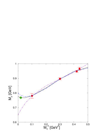
Figure 4: The rho meson mass as a function of the light quark mass, $M_{\pi}^{2}\sim(m_{u}+m_{d})$. The solid (dot-dashed) line(s) refers to fit 1 (2,3) as described in the text. The lattice data are from CP-PACS CPPACS . The diamond denotes the physical rho mass.

The corresponding curves are shown in Fig. 4. To get a better handle on the theoretical uncertainty, we also allow the fits to stay within the theoretical uncertainty of the lowest point at $M_{\pi}^{2}=0.1\,$GeV², as shown in Fig. 5. If we insist again on naturalness of the coupling constants, we can bound the $\rho$-mass in the chiral limit by

$$650~{}{\rm MeV}\leq M_{\rho}^{0}\leq 800~{}{\rm MeV}~{}.$$ (12.7)

These results are similar to what was found in the pioneering work in Ref. Ausrho , but they are less model-dependent. The range for $M_{\rho}^{0}$ is also consistent with the numbers derived by Bijnens and collaborators in their study of vector mesons in chiral perturbation theory bijnens . It would be interesting to extend these studies in two directions, first to include also more recent lattice data and second to try to give more stringent limits on the combinations of LECs by incorporating more phenomenological constraints.

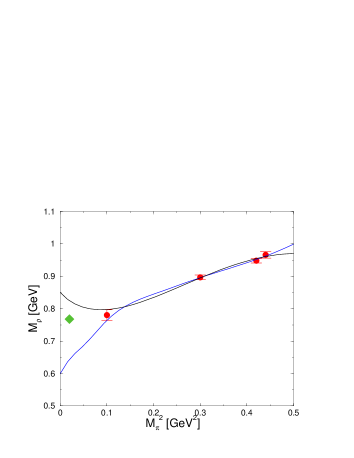
Figure 5: The rho meson mass as a function of the pion mass: Theoretical uncertainty as described in the text. For further notations, see Fig. 4.

The quark mass expansion of the $\rho$-mass Eq.(12.6) allows one to deduce the corresponidng $\sigma$–term,

$$\sigma_{\pi\rho}=\hat{m}\,\frac{\partial M_{\rho}}{\partial\hat{m}}=M_{\pi}^{2}\,\frac{\partial M_{\rho}}{\partial M_{\pi}^{2}}~{},$$ (12.8)

with $\hat{m}$ the average light quark mass. From the numbers collected in Table 1, we find

$$-1.9\,M_{\pi}^{2}\leq\sigma_{\pi\rho}\leq 1.5\,M_{\pi}^{2}~{}.$$ (12.9)

This shows again that the rho as a massive particle has a very different quark mass expansion than the pion, where $\sigma_{\pi}\simeq M_{\pi}^{2}$ GL1 . In magnitude, the rho $\sigma$-term is similar to the pion-nucleon one, $\sigma_{\pi N}\simeq 45\,$MeV.

13 Summary and outlook

In this paper, we have considered chiral perturbation theory in the presence of vector and axial-vector mesons (spin-1) fields and presented an extension of the infrared regularization scheme originally developed for baryon chiral perturbation theory. The pertinent results of this investigation can be summarized as follows:

• The most economic way to deal with vector mesons in chiral perturbation theory is to utilize the antisymmetric tensor field formulation as stressed in NuB . When vector mesons appear in tree graphs only, calculations are straightforward as summarized in Sect. 2 and App. A. Of course, other formulations like the vector field approach can also be used, see App. B,C.

• When vector mesons appear in loops, the appearance of the large mass scale complicates the power counting, as discussed in Sect. 3 and Sect. 4. In essence, loop diagrams pick up large contributions when the loop momentum is close to the vector meson mass. To the contrary, the contribution from the soft poles (momenta of the order of the pion mass) that leads to the interesting chiral terms of the low-energy EFT (chiral logs and alike) obeys power counting. We have briefly summarized the method proposed in Tang to extract the ‘soft pole’ contribution from one-loop integrals.

• The standard case of infrared regularization BL , where the heavy particle line is conserved in the (one-loop) graphs is recapitulated in Sect. 5. For these cases a very elegant splitting of a Feynman parameter integral allows to unambigouosly separate the infrared singular from the regular part, cf. Eq.(5).

• In the case of spin-1 fields, new classes of self-energy graphs appear. The case for lines with small external momenta but a vector meson line appearing inside the diagram in analyzed in Sect. 6 and the singularity structure of the corresponding integrals is discussed in Sect. 7. In Sect. 8 the infrared singular part for such types of integrals is explicitly constructed, cf. Eq. (8.4). As explicit examples, the Goldstone boson self-energy and the triangle diagram are worked out in Sect. 9 and Sect. 10, respectively.

• A different type of one-loop graphs appears in the vector meson self-energy, where only light particles (Goldstone bosons) run in the loop. This is discussed in detail in Sect. 11, where the corresponding infrared singular part is extracted, see Eq. (11.7), and the contribution to the vector meson mass is worked out. We briefly discuss the problems related to the imaginary part of such type of diagrams.

• As an application, we consider the pion mass dependence of the $\rho$-meson mass in Sect. 12. We show that there are many contributions with unknown LECs, still one is able to derive a compact formula for $M_{\rho}(M_{\pi})$, see Eq. (12.6). We analyze existing lattice data CPPACS and conclude that the $\rho$-meson mass in the chiral limit is bounded between 650 and 800 MeV. We have also discussed the $\pi\rho$ sigma term.

The methods outlined here can be applied to many interesting problems, for example one could systematically analyze vector meson effects on Goldstone properties like form factors or polarizabilities or extend these considerations to systems including baryons (for a first step see e.g. BM95 ).

Appendix A Tensor field approach

In this appendix, we briefly discuss the representation of spin-1 particles in terms of antisymmetric tensor fields, following closely Appendix A of NuB .

As an antisymmetric tensor field, $W_{\mu\nu}$ has six degrees of freedom, whereas a massive vector field only has three. Loosely speaking, there are two spin-1 fields ’hidden’ in a general antisymmetric tensor field approach (corresponding to a reducible representation of the rotation group). To make this clear, we decompose the tensor field $W_{\mu\nu}$ (in momentum space)

$$W_{\mu\nu}=(W-PWP)_{\mu\nu}+(PWP)_{\mu\nu}\equiv W^{L}_{\mu\nu}+W^{T}_{\mu\nu},$$ (A.1)

where the matrix $P$ is the projector

$$P_{\mu\nu}=g_{\mu\nu}-\frac{p_{\mu}p_{\nu}}{p^{2}},$$ (A.2)

and $p_{\mu}$ is the momentum four-vector associated with the tensor field. Because of the projector property of $P$, we have

$$p^{\mu}W_{\mu\nu}^{T}=0,$$

giving 4 conditions for six degrees of freedom, but one condition is redundant due to the antisymmetry property of $W_{\mu\nu}$. So we are left with $6-3=3$ degrees of freedom for $W^{T}$, and therefore also for $W^{L}$.

Inserting the above decomposition in the general form of an action principle for antisymmetric tensor fields NuB ,

$$\tilde{S}_{W} = \int d^{4}x\bigl{\{}(a-2b)\partial^{\mu}W_{\mu\nu}\partial_{\rho}W^{\rho\nu}+b\partial^{\rho}W_{\mu\nu}\partial_{\rho}W^{\mu\nu}$$ (A.3)

$$\qquad\qquad+cW_{\mu\nu}W^{\mu\nu}\bigr{\}}~{},$$

with arbitrary parameters $a,b$, and $c\not=0$, and using

$$W_{\mu\nu}^{L}W^{\mu\nu}_{T}=0,$$

which is easily verified by a direct calculation, we see that the action splits in two terms:

$$\tilde{S}_{W}=S_{W_{L}}+S_{W_{T}},$$ (A.4)

where

$$S_{W_{L}} = \int d^{4}x\bigl{(}a\partial^{\mu}W_{\mu\nu}^{L}\partial_{\rho}W^{\rho\nu}_{L}+cW_{\mu\nu}^{L}W^{\mu\nu}_{L}\bigr{)},$$

$$S_{W_{T}} = \int d^{4}x\bigl{(}b\partial^{\rho}W_{\mu\nu}^{T}\partial_{\rho}W^{\mu\nu}_{T}+cW_{\mu\nu}^{T}W^{\mu\nu}_{T}\bigr{)}.$$

Therefore, the path integral can also be factored:

$$\int[dW]e^{i\tilde{S}_{W}}=\int[dW_{L}]e^{iS_{W_{L}}}\int[dW_{T}]e^{iS_{W_{T}}}.$$ (A.5)

In the rest frame, this decomposition corresponds to

$$[dW]=[dW_{L}][dW_{T}]=\prod_{i=1}^{3}[dW_{0i}]\prod_{i<j}^{3}[dW_{ij}].$$

Following NuB , we choose $b=0$, so that the second path integral becomes an unimportant constant (from the viewpoint of the classical action, $W_{T}$ becomes a non-propagating field). For $a=0$, in contrast, $W_{L}$ would be ’frozen’ in this way. Choosing, furthermore,

$$a=-\frac{1}{2},\qquad c=\frac{M_{V}^{2}}{4},$$ (A.6)

and dropping the letter $L$, the massive vector field is described by

$$\int[dW]e^{iS_{W}} = \int[dW]{\rm exp}\biggl{\{}i\int d^{4}x\ (-\frac{1}{2}\partial^{\mu}W_{\mu\nu}\partial_{\rho}W^{\rho\nu}$$ (A.7)

$$\qquad\qquad+\frac{M_{V}^{2}}{4}W_{\mu\nu}W^{\mu\nu})\}.$$

Without invalidating the above argument, we can also add a coupling linear in $W$, of the form

$$-\frac{1}{4}J_{\mu\nu}W^{\mu\nu},$$

with some external antisymmetric current $J_{\mu\nu}$. Since we do not use couplings quadratic in the tensor field in this work, we will not attempt to extend the given argument to Lagrangians including such more complicated interaction terms.

Appendix B Vector field approach

One can now ask how much the results obtained from calculations similar to the ones in the main body of the text depend on the description in terms of an antisymmetric tensor field. Of course a dependence of that kind is not wanted for physical observables!

What happens if one uses a more conventional vector field approach for the description of the vector mesons? The Lagrangian for a massive vector field $V_{\mu}$ is well known:

$${\mathcal{L}}_{V}^{kin}=-\frac{1}{4}\langle V_{\mu\nu}V^{\mu\nu}\rangle+\frac{1}{2}M_{V}^{2}\langle V_{\mu}V^{\mu}\rangle$$ (B.1)

where $V_{\mu\nu}$ is the field strength tensor associated with $V_{\mu}$,

$$V_{\mu\nu}=\nabla_{\mu}V_{\nu}-\nabla_{\nu}V_{\mu}.$$

The corresponding vector field propagator (in momentum space) reads

$$G_{\mu\nu}(k)=(-i)\frac{\biggl{(}g_{\mu\nu}-\frac{k_{\mu}k_{\nu}}{M_{V}^{2}}\biggr{)}}{k^{2}-M_{V}^{2}+i\epsilon}.$$ (B.2)

If one now tries to write down interaction terms in analogy to the ones given before, it is seen that they are all $O(p^{3})$, giving a resonance exchange diagram of $O(p^{6})$ in contrast to the $O(p^{4})$ result derived with the antisymmetric tensor field description. In particular, the interaction terms are

$${\mathcal{L}}_{V}^{int}=-\frac{f_{V}}{2\sqrt{2}}\langle F^{+}_{\mu\nu}V^{\mu\nu}\rangle-\frac{ig_{V}}{2\sqrt{2}}\langle[u_{\mu},u_{\nu}]V^{\mu\nu}\rangle.$$ (B.3)

Here $f_{V}$ and $g_{V}$ are new coupling constants, and the minus sign is a pure convention. This interaction looks very much like Eq. (2.11), but note that the tensor $V_{\mu\nu}$ contains, from its definition, an additional derivative giving the interaction the order $O(p^{3})$ instead of $O(p^{2})$. The form factor contribution derived with this interaction is of higher order than the result of the last section and does not agree with experiment. If we had started with a vector field description for vector mesons, we might have concluded that the vector meson contribution is less important than suggested, for example, by a dispersive analysis. This problem was already solved in Eck , we simply repeat here some of salient ingredients in a slightly different way.

The mathematical relation between the two variants of the theory was worked out in Eck by imposing e.g. the large momentum transfer constraints on the pion vector form factor. In App. C, we argue that the Lagrangians

$${\mathcal{L}}_{W}^{kin}-\frac{1}{4}\langle J_{\mu\nu}W^{\mu\nu}\rangle$$ (B.4)

and

$${\mathcal{L}}_{V}^{kin}+\frac{1}{4M_{V}}\langle J_{\mu\nu}V^{\mu\nu}\rangle-\frac{1}{16M_{V}^{2}}\langle J_{\mu\nu}J^{\mu\nu}\rangle$$ (B.5)

indeed give equivalent theories on the level of the path integrals, when $J_{\mu\nu}$ are some traceless hermitian sources. This equivalence is achieved by simply integrating out the field $W_{\mu\nu}$, which leads to the appearance of contact terms quadratic in the source. The source terms we use are

$$J_{\mu\nu}=-\sqrt{2}(F_{V}F^{+}_{\mu\nu}+iG_{V}[u_{\mu},u_{\nu}])$$

(compare Eq. (2.11)) and, assuming the validity of the path-integral argument for the equivalence, we draw the conclusion that equivalence leads to

$$f_{V}=\frac{F_{V}}{M_{V}},\qquad g_{V}=\frac{G_{V}}{M_{V}}~{},$$ (B.6)

in perfect agreement with Ref. Eck . Furthermore, since the $V_{\mu\nu}$- couplings are of $O(p^{3})$, we conclude that vector meson exchange to lowest order $O(p^{4})$ can be represented by the contact terms

$$\frac{1}{16M_{V}^{2}}\langle J_{\mu\nu}J^{\mu\nu}\rangle = \left<-\frac{G_{V}^{2}}{8M_{V}^{2}}[u_{\mu},u_{\nu}][u^{\mu},u^{\nu}]\right.$$

$$+ \left.\frac{F_{V}^{2}}{8M_{V}^{2}}F^{+}_{\mu\nu}F^{\mu\nu}_{+}+\frac{iF_{V}G_{V}}{4M_{V}^{2}}F^{+}_{\mu\nu}[u^{\mu},u^{\nu}]\right>~{}.$$

Using the definition of the objects $u_{\mu}$ and $F^{+}_{\mu\nu}$ and standard trace relations, the contact terms can be written as

$$-\frac{1}{16M_{V}^{2}}\langle J_{\mu\nu}J^{\mu\nu}\rangle = L^{V}_{1}P_{1}+L^{V}_{2}P_{2}+L^{V}_{3}P_{3}$$

$$+L^{V}_{9}P_{9}+L^{V}_{10}P_{10}+H^{V}_{11}P_{11}~{},$$

with $P_{i}$ the structures of the fourth order meson Lagrangian GL2 and furthermore

$$L^{V}_{1} = \frac{G_{V}^{2}}{8M_{V}^{2}}~{},\qquad L^{V}_{2}=2L^{V}_{1}~{},\quad L^{V}_{3}=-6L^{V}_{1}$$

$$L^{V}_{9} = \frac{F_{V}G_{V}}{2M_{V}^{2}}~{},\quad L^{V}_{10}=-\frac{F_{V}^{2}}{4M_{V}^{2}}~{},\quad H^{V}_{11}=-\frac{F_{V}^{2}}{8M_{V}^{2}}~{}.$$

Appendix C Duality transformation

The action for an antisymmetric tensor field $W_{\mu\nu}$ is

$$S_{W}=\int d^{4}x\ {\mathcal{L}}_{W}$$ (C.1)

Note that $W_{\mu\nu}$ now stands for the field $W_{\mu\nu}^{L}$, having three degrees of freedom, as discussed in App. A. Now let us modify this action by a term containing a vector field $V_{\mu}$:

$${\mathcal{L}}_{V,W}={\mathcal{L}}_{W}-\frac{1}{4}J_{\mu\nu}W^{\mu\nu}+\frac{M_{V}^{2}}{2}\biggl{(}V_{\mu}-\frac{1}{M_{V}}\partial^{\nu}W_{\nu\mu}\biggr{)}^{2}~{}.$$ (C.2)

We have also added a source term linear in $W_{\mu\nu}$. The equations of motion (e.o.m.) following from this Lagrangian are

$$W_{\mu\nu}+\frac{1}{M_{V}}(\partial_{\mu}V_{\nu}-\partial_{\nu}V_{\mu}) = \frac{1}{2M_{V}^{2}}J_{\mu\nu},$$ (C.3)

$$V_{\mu}-\frac{1}{M_{V}}(\partial^{\sigma}W_{\sigma\mu}) = 0.$$ (C.4)

Substituting $V_{\mu}$ from the second equation into the first one, the latter becomes the ’old’ e.o.m. following from $L_{W}-\frac{1}{4}J\cdot W$ alone. So on the classical level, the additional squared term does not change anything.

Considering now path integrals, we deduce by a Gaussian integration over $V$ that

$$\int[dW]e^{i\int d^{4}x(L_{W}-\frac{1}{4}J_{\mu\nu}W^{\mu\nu})}\sim\int[dW]\int[dV]e^{i\int d^{4}xL_{V,W}},$$ (C.5)

where the ’$\sim$’ means ’up to a constant factor’. It must be noted here that the vector field $V$ should be treated like $W$, that is using a constraint to eliminate one degree of freedom. On the classical level, the second e.o.m. says that $V$ has the same number of degrees of freedom as $W$, i.e. three d.o.f. Contributions of the path integral over $V$ deviating from this e.o.m are exponentially damped like $e^{-x^{2}}$ because of the form of the squared term in $L_{V,W}$. Using a constraint on $V$, we will get just another constant prefactor as long as this constraint is linear in the field.

If we now recklessly interchange the order of integrations on the right-hand-side of Eq. (C.5), define

$$V_{\mu\nu}=\partial_{\mu}V_{\nu}-\partial_{\nu}V_{\mu},$$

and do the $W$-integration, we get

$$\int[dW]e^{i\int d^{4}x\ (L_{W}-\frac{1}{4}J_{\mu\nu}W^{\mu\nu})}$$

$$\sim \int[dV][dW]\exp\biggl{\{}i\int d^{4}x\ \biggl{(}\frac{1}{4}M_{V}^{2}W_{\mu\nu}W^{\mu\nu}-\frac{1}{4}J_{\mu\nu}W^{\mu\nu}$$

$$\qquad\qquad\qquad\qquad\qquad+\frac{M_{V}^{2}}{2}V_{\mu}V^{\mu}+\frac{M_{V}}{2}V_{\mu\nu}W^{\mu\nu}\biggr{)}\biggr{\}}$$

$$\sim \int[dV]\exp\biggl{\{}i\int d^{4}x\ \biggl{(}-\frac{1}{4}V_{\mu\nu}V^{\mu\nu}+\frac{M_{V}^{2}}{2}V_{\mu}V^{\mu}$$

$$\qquad\qquad\qquad\qquad+\frac{1}{4M_{V}}J_{\mu\nu}V^{\mu\nu}-\frac{1}{16M_{V}^{2}}J_{\mu\nu}J^{\mu\nu}\biggr{)}\biggr{\}}~{}.$$

This corresponds to a conventional vector field Lagrangian, together with contact terms of the form

$$-\frac{1}{16M_{V}^{2}}J_{\mu\nu}J^{\mu\nu}.$$

If the tensor field $W$ is given in the matrix notation of Eq. (2.6), which implies that one has to take the (flavor) trace of every term in the Lagrangian $L_{W}$, the source term linear in the field $W_{\mu\nu}^{a}$ can be taken as

$$-\frac{1}{4}\langle W_{\mu\nu}J^{\mu\nu}\rangle=-\frac{1}{4\sqrt{2}}W_{\mu\nu}^{a}\langle T^{a}J^{\mu\nu}\rangle.$$

If $J_{\mu\nu}$ is traceless and hermitian (which is the case for the couplings we consider in Eq.(2.11)), we produce the contact terms

$$\biggl{(}\frac{1}{16M_{V}^{2}}\biggr{)}\frac{1}{\sqrt{2}}\langle J_{\mu\nu}T^{a}\rangle\frac{1}{\sqrt{2}}\langle J^{\mu\nu}T^{a}\rangle=\frac{1}{16M_{V}^{2}}\langle J_{\mu\nu}J^{\mu\nu}\rangle,$$

which justifies the form of the contact terms given in the preceding appendix.

A path-integral approach to show the duality of the antisymmetric tensor field and the vector field description has also been presented in Bij , but the approach used here is shorter. In principle, we have not done much more than a Legendre transformation to change variables from $\partial W$ to $V$. The $W$-field has been integrated out, leaving as a ’souvenir’ only the contact terms. As in the foregoing Appendix, we do not attempt to include also more complicated coupling terms in such a transformation, with the excuse that in this work the contact terms are only needed for the linear interaction of Eq. (2.11).

Appendix D Loop integrals

In this Appendix we treat the reduction of general loop integrals to linear combinations of scalar loop integrals. The scalar loop integrals $I_{\phi}$ and $I_{V}$ have been defined in Eqs.(9.5) and (9.6), respectively, while $I_{V\phi}$ was defined in Eq. (5.1). Writing $q^{2}=(q^{2}-M_{V}^{2})+M_{V}^{2}$, one derives

$$i\int\frac{d^{d}q}{(2\pi)^{d}}\frac{q^{2}}{(q^{2}-M_{V}^{2})((q-p)^{2}-M_{\phi}^{2})}$$

$$=I_{\phi}+M_{V}^{2}I_{V\phi}(p).$$ (D.1)

Moreover, by Lorentz invariance, we must have

$$i\int\frac{d^{d}q}{(2\pi)^{d}}\frac{q^{\mu}}{(q^{2}-M_{V}^{2})((q-p)^{2}-M_{\phi}^{2})}=p^{\mu}S,$$ (D.2)

because there is no other four-vector than $p^{\mu}$ available here. The scalar $S$ can be found by contracting with $p_{\mu}$:

$$S = \frac{i}{2p^{2}}\int\frac{d^{d}q}{(2\pi)^{d}}\frac{q^{2}+p^{2}-(q-p)^{2}}{(q^{2}-M_{V}^{2})((q-p)^{2}-M_{\phi}^{2})}$$ (D.3)

$$= \frac{1}{2p^{2}}(I_{\phi}-I_{V}+(M_{V}^{2}-M_{\phi}^{2}+p^{2})I_{V\phi}).$$

Using both results together, we can compute

$$i\int\frac{d^{d}q}{(2\pi)^{d}}\frac{(p\cdot q)q^{\mu}}{(q^{2}-M_{V}^{2})((q-p)^{2}-M_{\phi}^{2})}$$

$$=\frac{p^{\mu}}{4p^{2}}(a_{\phi}I_{\phi}+a_{V}I_{V}+a_{V\phi}I_{V\phi}),$$ (D.4)

where the coefficients are given by

$$a_{\phi} = M_{V}^{2}-M_{\phi}^{2}+3p^{2},$$

$$a_{V} = M_{\phi}^{2}-M_{V}^{2}-p^{2}~{},~{}~{}a_{V\phi}=a_{V}^{2}.$$ (D.5)

These results so far are already sufficient to arrive at the decomposition of Eq. (9.3) for $I_{\Sigma}$. Another useful result is also derived using Lorentz invariance:

$$i\int\frac{d^{d}q}{(2\pi)^{d}}\frac{q^{\mu}q^{\nu}}{(q^{2}-M_{\phi}^{2})((q-p)^{2}-M_{\phi}^{2})}$$

$$=g^{\mu\nu}A(p)+\frac{p^{\mu}p^{\nu}}{p^{2}}B(p)~{}.$$ (D.6)

The coefficients can be found by contracting with $g_{\mu\nu}$ and $p_{\mu}$, using the above results and $g_{\mu\nu}g^{\mu\nu}=d$ :

$$(d-1)A(p) = \frac{1}{2}I_{\phi}+\frac{1}{4}(4M_{\phi}^{2}-p^{2})I_{\phi\phi}(p)$$ (D.7)

$$(d-1)B(p) = \biggl{(}\frac{d}{2}-1\biggr{)}I_{\phi}+\biggl{(}\frac{d}{4}p^{2}-M_{\phi}^{2}\biggr{)}I_{\phi\phi}(p).$$

Here the integral $I_{\phi\phi}(p)$ is obtained from $I_{V\phi}(p)$ by substituting $M_{\phi}$ for $M_{V}$.

The last result we have to derive is the integral $I_{\Delta}^{\tau}(p,k)$, which we only need for on-shell kinematics , $p^{2}=k^{2}=M_{\phi}^{2}$. Using the algebraic decomposition

$$\frac{4(p\cdot k)q^{2}-4(p\cdot q)(k\cdot q)}{(q^{2}-M_{V}^{2})(q^{2}-2q\cdot p)(q^{2}-2q\cdot k)}$$

$$=\frac{4(p\cdot k)M_{V}^{2}-M_{V}^{4}}{(q^{2}-M_{V}^{2})(q^{2}-2q\cdot p)(q^{2}-2q\cdot k)}$$

$$+\frac{4(p\cdot k)-q^{2}-M_{V}^{2}}{(q^{2}-2q\cdot p)(q^{2}-2q\cdot k)}-\frac{1}{q^{2}-M_{V}^{2}}$$

$$+\frac{1}{q^{2}-2q\cdot p}+\frac{1}{q^{2}-2q\cdot k}$$

$$+\frac{M_{V}^{2}}{(q^{2}-M_{V}^{2})(q^{2}-2q\cdot p)}$$

$$+\frac{M_{V}^{2}}{(q^{2}-M_{V}^{2})(q^{2}-2q\cdot k)}~{},$$

the results obtained in this appendix enable us to calculate

$$I^{\tau}_{\Delta}(p,k)=$$

$$i\int\frac{d^{d}q}{(2\pi)^{d}}\frac{(p+k-2q)^{\tau}((p\cdot k)q^{2}-(p\cdot q)(k\cdot q))}{(q^{2}-M_{V}^{2})((q-p)^{2}-M_{\phi}^{2})((q-k)^{2}-M_{\phi}^{2})}$$

$$=(p+k)^{\tau}(d_{V\phi\phi}I_{V\phi\phi}(p,k)+d_{V\phi}I_{V\phi}$$

$$\quad\quad+d_{\phi\phi}I_{\phi\phi}(k-p)+d_{\phi}I_{\phi}+d_{V}I_{V})~{}.$$ (D.8)

The coefficients are given by

$$4d_{V\phi\phi} = \frac{(M_{\phi}^{2}-M_{V}^{2}+(p\cdot k))(4(p\cdot k)M_{V}^{2}-M_{V}^{4})}{M_{\phi}^{2}+(p\cdot k)},$$

$$4d_{V\phi} = \frac{2M_{\phi}^{2}M_{V}^{2}-M_{V}^{4}}{M_{\phi}^{2}}-\frac{M_{V}^{4}-4(p\cdot k)M_{V}^{2}}{M_{\phi}^{2}+(p\cdot k)},$$

$$4d_{\phi\phi} = \frac{M_{\phi}^{2}+(p\cdot k)}{d-1}-\frac{4(p\cdot k)M_{V}^{2}-M_{V}^{4}}{M_{\phi}^{2}+(p\cdot k)},$$

$$4d_{\phi} = \frac{1}{d-1}-\frac{M_{V}^{2}}{M_{\phi}^{2}},~{}~{}4d_{V}=\frac{M_{V}^{2}}{M_{\phi}^{2}}-1.$$ (D.9)

We remind the reader that this is valid only for $p^{2}=k^{2}=M_{\phi}^{2}$. For this case, we have $I_{V\phi}(k)=I_{V\phi}(p)\equiv I_{V\phi}\,$.

References

- (1) J. Gasser and H. Leutwyler, Annals Phys. 158 (1984) 142.
- (2) J. Gasser and H. Leutwyler, Nucl. Phys. B 250 (1985) 465.
- (3) S. Weinberg, PhysicaA 96 (1979) 327.
- (4) U.-G. Meißner, Rept. Prog. Phys. 56 (1993) 903 [arXiv:hep-ph/9302247].
- (5) A. Pich, Rept. Prog. Phys. 58 (1995) 563 [arXiv:hep-ph/9502366].
- (6) G. Ecker, Prog. Part. Nucl. Phys. 35 (1995) 1 [arXiv:hep-ph/9501357].
- (7) V. Bernard, N. Kaiser and U.-G. Meißner, Int. J. Mod. Phys. E 4 (1995) 193 [arXiv:hep-ph/9501384].
- (8) S. Scherer, Adv. in Nucl. Phys. 27 (2003) 277 [arXiv:hep-ph/0210398].
- (9) H. Leutwyler, Annals Phys. 235 (1994) 165 [arXiv:hep-ph/9311274].
- (10) S. Weinberg, in Lecture Notes in Physics, Vol. 452 (Springer Verlag, Heidelberg 1995) [arXiv:hep-ph/9412326].
- (11) U.-G. Meißner, Phys. Rept. 161 (1988) 213.
- (12) M. Bando, T. Kugo and K. Yamawaki, Phys. Rept. 164 (1988) 217.
- (13) G. Ecker, J. Gasser, A. Pich and E. de Rafael, Nucl. Phys. B 321 (1989) 311.
- (14) J. F. Donoghue, C. Ramirez and G. Valencia, Phys. Rev. D 39 (1989) 1947.
- (15) G. Ecker, J. Gasser, H. Leutwyler, A. Pich and E. de Rafael, Phys. Lett. B 223 (1989) 425.
- (16) J. Gasser, M. E. Sainio and A. Svarc, Nucl. Phys. B 307 (1988) 779.
- (17) E. Jenkins and A. V. Manohar, Phys. Lett. B 255 (1991) 558.
- (18) V. Bernard, N. Kaiser, J. Kambor and U.-G. Meißner, Nucl. Phys. B 388 (1992) 315.
- (19) H. B. Tang, arXiv:hep-ph/9607436; P. J. Ellis and H. B. Tang, Phys. Rev. C 57 (1998) 3356 [arXiv:hep-ph/9709354].
- (20) T. Becher and H. Leutwyler, Eur. Phys. J. C 9 (1999) 643 [arXiv:hep-ph/9901384].
- (21) T. Fuchs, J. Gegelia, G. Japaridze and S. Scherer, Phys. Rev. D 68 (2003) 056005 [arXiv:hep-ph/0302117]; M. R. Schindler, J. Gegelia and S. Scherer, Nucl. Phys. B 682 (2004) 367 [arXiv:hep-ph/0310207].
- (22) E. Jenkins, A. V. Manohar and M. B. Wise, Phys. Rev. Lett. 75, 2272 (1995) [arXiv:hep-ph/9506356].
- (23) B. Borasoy and U.-G. Meißner, Int. J. Mod. Phys. A 11, 5183 (1996) [arXiv:hep-ph/9511320].
- (24) R. Urech, Phys. Lett. B 355 (1995) 308 [arXiv:hep-ph/9504238].
- (25) J. Bijnens and P. Gosdzinsky, Phys. Lett. B 388 (1996) 203 [arXiv:hep-ph/9607462]; J. Bijnens, P. Gosdzinsky and P. Talavera, Nucl. Phys. B 501 (1997) 495 [arXiv:hep-ph/9704212]; J. Bijnens, P. Gosdzinsky and P. Talavera, JHEP 9801 (1998) 014 [arXiv:hep-ph/9708232]; J. Bijnens, P. Gosdzinsky and P. Talavera, Phys. Lett. B 429 (1998) 111 [arXiv:hep-ph/9801418].
- (26) V. Cirigliano, G. Ecker, H. Neufeld and A. Pich, JHEP 0306 (2003) 012 [arXiv:hep-ph/0305311]; P. D. Ruiz-Femenia, A. Pich and J. Portoles, JHEP 0307 (2003) 003 [arXiv:hep-ph/0306157]; I. Rosell, J. J. Sanz-Cillero and A. Pich, JHEP 0408 (2004) 042 [arXiv:hep-ph/0407240].
- (27) M. Harada and K. Yamawaki, Phys. Rept. 381 (2003) 1 [arXiv:hep-ph/0302103].
- (28) T. Fuchs, M. R. Schindler, J. Gegelia and S. Scherer, Phys. Lett. B 575 (2003) 11 [arXiv:hep-ph/0308006]; D. Djukanovic, M. R. Schindler, J. Gegelia, G. Japaridze and S. Scherer, Phys. Rev. Lett. 93, 122002 (2004) [arXiv:hep-ph/0407239].
- (29) B. Kubis and U.-G. Meißner, Nucl. Phys. A 679 (2001) 698 [arXiv:hep-ph/0007056].
- (30) D. Lehmann and G. Prezeau, Phys. Rev. D 65 (2002) 016001 [arXiv:hep-ph/0102161].
- (31) D. B. Leinweber and T. D. Cohen, Phys. Rev. D 49 (1994) 3512 [arXiv:hep-ph/9307261].
- (32) D. B. Leinweber, A. W. Thomas, K. Tsushima and S. V. Wright, Phys. Rev. D 64 (2001) 094502 [arXiv:hep-lat/0104013].
- (33) S. Aoki et al. [CP-PACS Collaboration], Phys. Rev. D 60 (1999) 114508 [arXiv:hep-lat/9902018].
- (34) N. Fettes, U.-G. Meißner and S. Steininger, Nucl. Phys. A 640 (1998) 199 [arXiv:hep-ph/9803266].
- (35) P. Büttiker and U.-G. Meißner, Nucl. Phys. A 668 (2000) 97 [arXiv:hep-ph/9908247].
- (36) J. Bijnens and E. Pallante, Mod. Phys. Lett. A 11 (1996) 1069 [arXiv:hep-ph/9510338].