hep-ph/0411216 CERN–PH–TH/2004-220

DCPT/04/146, IPPP/04/73 UMN–TH–2326/04, FTPI–MINN–04/40

Indirect Sensitivities to the Scale of Supersymmetry

John Ellis¹, Sven Heinemeyer¹, Keith A. Olive² and Georg Weiglein^3
1TH Division, Physics Department, CERN, Geneva, Switzerland
²William I. Fine Theoretical Physics Institute,
University of Minnesota, Minneapolis, MN 55455, USA
³Institute for Particle Physics Phenomenology, University of Durham,
Durham DH1 3LE, UK
Abstract

Precision measurements, now and at a future linear electron-positron collider (ILC), can provide indirect information about the possible scale of supersymmetry. We illustrate the present-day and possible future ILC sensitivities within the constrained minimal supersymmetric extension of the Standard Model (CMSSM), in which there are three independent soft supersymmetry-breaking parameters $m_{1/2},m_{0}$ and $A_{0}$. We analyze the present and future sensitivities separately for $M_{W}$, $\sin^{2}\theta_{\mathrm{eff}}$, $(g-2)_{\mu}$, ${\rm BR}(b\to s\gamma)$, ${\rm BR}(B_{s}\to\mu^{+}\mu^{-})$, $M_{h}$ and Higgs branching ratios. We display the observables as functions of $m_{1/2}$, fixing $m_{0}$ so as to obtain the cold dark matter density allowed by WMAP and other cosmological data for specific values of $A_{0}$, $\tan\beta$ and $\mu>0$. In a second step, we investigate the combined sensitivity of the currently available precision observables, $M_{W}$, $\sin^{2}\theta_{\mathrm{eff}}$, $(g-2)_{\mu}$ and ${\rm BR}(b\to s\gamma)$, by performing a $\chi^{2}$ analysis. The current data are in very good agreement with the CMSSM prediction for $\tan\beta=10$, with a clear preference for relatively small values of $m_{1/2}\sim 300$ GeV. In this case, there would be good prospects for observing supersymmetry directly at both the LHC and the ILC, and some chance already at the Tevatron collider. For $\tan\beta=50$, the quality of the fit is worse, and somewhat larger $m_{1/2}$ values are favoured. With the prospective ILC accuracies the sensitivity to indirect effects of supersymmetry greatly improves. This may provide indirect access to supersymmetry even at scales beyond the direct reach of the LHC or the ILC.

CERN–PH–TH/2004-220

November 2004

1 Introduction

Measurements at low energies may provide interesting indirect information about the masses of particles that are too heavy to be produced directly. A prime example is the use of precision electroweak data from LEP, the SLC, the Tevatron and elsewhere to predict (successfully) the mass of the top quark and to provide an indication of the possible mass of the hypothetical Higgs boson [1]. Predicting the masses of supersymmetric particles is much more difficult than for the top quark or even the Higgs boson, because the renormalizability of the Standard Model and the decoupling theorem imply that many low-energy observables are insensitive to heavy sparticles. Nevertheless, present data on observables such as $M_{W}$, $\sin^{2}\theta_{\mathrm{eff}}$, $(g-2)_{\mu}$ and ${\rm BR}(b\to s\gamma)$ already provide interesting information on the scale of supersymmetry (SUSY), as we discuss in this paper, and have a great potential in view of prospective improvements of experimental and theoretical accuracies.

In the future, a linear $e^{+}e^{-}$ collider (ILC) will be the best available tool for making many precision measurements [2]. It is important to understand what information ILC measurements may provide about supersymmetry, both for the part of the spectrum directly accessible at the LHC or the ILC and for sparticles that would be too heavy to be produced directly. Comparing the indirect indications with the direct measurements would be an important consistency check on the theoretical framework of supersymmetry.

Improved and more complete calculations of the supersymmetric contributions to a number of low-energy observables such as $M_{W}$ and $\sin^{2}\theta_{\mathrm{eff}}$ have recently become available (see the discussion in Sect. 3 below). These, combined with estimates of the experimental accuracies attainable at the ILC and future theoretical uncertainties from unknown higher-order corrections, make now an opportune moment to assess the likely sensitivities of ILC measurements.

There have been many previous studies of the sensitivity of low-energy observables to the scale of supersymmetry, including, for example, the precision electroweak observables [3, 4, 5, 6, 7, 8, 9]. Such analyses are bedevilled by the large dimensionality of even the minimal supersymmetric extension of the Standard Model (MSSM), once supersymmetry-breaking parameters are taken into account. For this reason, simplifying assumptions that may be more or less well motivated are often made, so as to reduce the parameter space to a manageable dimensionality. Following many previous studies, we work here in the framework of the constrained MSSM (CMSSM), in which the soft supersymmetry-breaking scalar and gaugino masses are each assumed to be equal at some GUT input scale. In this case, the new independent MSSM parameters are just four in number: the universal gaugino mass $m_{1/2}$, the scalar mass $m_{0}$, the trilinear soft supersymmetry-breaking parameter $A_{0}$, and the ratio $\tan\beta$ of Higgs vacuum expectation values. The pseudoscalar Higgs mass $M_{A}$ and the magnitude of the Higgs mixing parameter $\mu$ can be determined by using the electroweak vacuum conditions, leaving the sign of $\mu$ as a residual ambiguity.

The non-discoveries of supersymmetric particles and the Higgs boson at LEP and other present-day colliders impose significant lower bounds on $m_{1/2}$ and $m_{0}$. An important further constraint is provided by the density of dark matter in the Universe, which is tightly constrained by WMAP and other astrophysical and cosmological data [10]. These have the effect within the CMSSM, assuming that the dark matter consists largely of neutralinos [11], of restricting $m_{0}$ to very narrow allowed strips for any specific choice of $A_{0}$, $\tan\beta$ and the sign of $\mu$ [12, 13]. Thus, the dimensionality of the supersymmetric parameter space is further reduced, and one may explore supersymmetric phenomenology along these ‘WMAP strips’, as has already been done for the direct detection of supersymmetric particles at the LHC and linear colliders of varying energies [14, 15, 16, 17, 18, 19]. A full likelihood analysis of the CMSSM planes incorporating uncertainties in the cosmological relic density was performed in Ref. [20]. The principal aim of this paper is to extend this analysis to indirect effects of supersymmetry.

We consider the following observables: the $W$ boson mass, $M_{W}$, the effective weak mixing angle at the $Z$ boson resonance, $\sin^{2}\theta_{\mathrm{eff}}$, the anomalous magnetic moment of the muon, $(g-2)_{\mu}$ and the rare $b$ decays ${\rm BR}(b\to s\gamma)$ and ${\rm BR}(B_{s}\to\mu^{+}\mu^{-})$, as well as the mass of the lightest ${\cal CP}$-even Higgs boson, $M_{h}$, and the Higgs branching ratios ${\rm BR}(h\to b\bar{b})/{\rm BR}(h\to WW^{*})$. We first analyze the sensitivity of each observable to indirect effects of supersymmetry, taking into account the present and prospective future experimental and theoretical uncertainties. We then investigate the combined sensitivity of those observables for which experimental determinations exist at present, i.e., $M_{W}$, $\sin^{2}\theta_{\mathrm{eff}}$, $(g-2)_{\mu}$ and ${\rm BR}(b\to s\gamma)$. We perform $\chi^{2}$ analyses both for fixed values of $A_{0}$ and for scans in the ($m_{1/2},A_{0}$) plane for $\tan\beta=10$ and 50 with $\mu>0$. We find a remarkably high sensitivity of the current data for the electroweak precision observables to the scale of supersymmetry. In the case $\tan\beta=10$, we find a preference for moderate values of $m_{1/2}\sim 300\,\,\mathrm{GeV}$, in which case sparticles should be observable at both the LHC and the ILC. In the case $\tan\beta=50$, the global fit is not so good, and low values of $m_{1/2}$ are not so strongly preferred. In order to investigate the possible future sensitivities we study the combined effect of all the above observables (except ${\rm BR}(B_{s}\to\mu^{+}\mu^{-})$, which is discussed separately). For this purpose we choose certain values of $(m_{1/2},A_{0})$ as assumed future ‘best-fit’ values (corresponding to the central values of the observables) and investigate the indirect constraints arising from the precision observables for prospective experimental and theoretical uncertainties.

In Section 2 of the paper we specify the WMAP strips and discuss their dependences on $A_{0}$ and the top-quark mass. We discuss in Section 3 the present and future sensitivities of the different precision observables to the scale of supersymmetry, represented by $m_{1/2}$ as one moves along different WMAP strips. In Section 4 we analyze the combined sensitivity of the precision observables for the present situation, and Section 5 presents the prospective combined sensitivity assuming the accuracies expected to become available at the ILC with its GigaZ option. Finally, Section 6 gives our conclusions. In most of the scenarios studied, even if it does not produce sparticles directly, the ILC will check the consistency of the CMSSM at the loop level and thereby provide valuable extra information beyond that obtainable with the LHC.

2 Supersymmetric dark matter and WMAP strips

It is well known that the lightest supersymmetric particle (LSP) is an excellent candidate for cold dark matter (CDM) [11], with a density that falls naturally within the range $0.094<\Omega_{\rm CDM}h^{2}<0.129$ favoured by a joint analysis of WMAP and other astrophysical and cosmological data [10]. Assuming that the cold dark matter is composed predominantly of LSPs, the uncertainty in the determination of $\Omega_{\rm CDM}h^{2}$ effectively reduces by one the dimensionality of the MSSM parameter space. Specifically, if one assumes that the soft supersymmetry-breaking gaugino masses $m_{1/2}$ and scalar masses $m_{0}$ are universal at some GUT input scale, as in the CMSSM studied here, the ($m_{1/2},m_{0}$) planes usually studied for fixed $A_{0}$, $\tan\beta$ and sign of $\mu$ are effectively reduced to narrow strips of limited thickness in $m_{0}$ for any given value of $m_{1/2}$ [12] and the other parameters.

These strips have been delineated and parametrized when $A_{0}=0$ for several choices of $\tan\beta$ for each sign of $\mu$, and the possible LHC and ILC phenomenology along these lines has been discussed [16]. As preliminaries to studying indirect sensitivities to the scale of supersymmetry along some of these WMAP strips, we first address a couple of physics issues. One is that the experimental central value of $m_{t}$ has changed since Ref. [16], from 174.3 GeV to 178.0 GeV [21], and the other is the dependence of the WMAP strips on $A_{0}$. The change in $m_{t}$ has a significant effect on the regions of CMSSM parameter space allowed, particularly in the focus-point region where the range of $m_{0}$ allowed by cosmology now starts above 4 TeV. In view of the high values of $m_{0}$ and the sensitivity to $m_{t}$ [22], we do not study the focus-point region further in this paper. There are also $m_{t}$- and $A_{0}$-dependent effects in the ‘funnels’ where neutralinos annihilate rapidly via the $H,A$ poles. These affect the dependence of $m_{0}$ on $m_{1/2}$ along the WMAP lines, as we now discuss in more detail. As explained below, because of the anomalous magnetic moment of the muon, we focus on cases with $\mu>0$.

Plotted in Fig. 1 is the region in the ($m_{1/2},m_{0}$) plane for fixed $\tan\beta,A_{0}$ and $\mu>0$ for which the relic density is in the WMAP range (the results of [9] are in qualitative agreement with Ref. [23]). We have applied cuts based on the lower limit to the Higgs mass, $b\to s\gamma$, and require that the LSP be a neutralino rather than the stau. The thin strips correspond to the relic density being determined by either the coannihilation between nearly degenerate $\tilde{\tau}$’s and $\chi$’s or, as seen at high $\tan\beta$, by rapid annihilation when $m_{\chi}\approx M_{A}/2$. We see in Fig. 1(a) that the WMAP strip for $\mu>0$ and $\tan\beta=10$ does not change much as $m_{t}$ is varied, reflecting the fact that the allowed strip is dominated by annihilation of the neutralino LSP $\chi$ with the lighter stau slepton ${\tilde{\tau}_{1}}$. The main effect of varying $m_{t}$ is that the truncation at low $m_{1/2}$, due to the Higgs mass constraint, becomes more important at low $m_{t}$. This effect is not visible in Fig. 1(b) for $\tan\beta=50$, where the cutoff at low $m_{1/2}$ is due to the $b\to s\gamma$ constraint, and rapid $\chi\chi\to A,H$ annihilation is important at large $m_{1/2}$. The allowed regions at larger $m_{1/2}$ vary significantly with $m_{t}$ when $\tan\beta=50$, because the $A,H$ masses and hence the rapid-annihilation regions are very sensitive to $m_{t}$ through the renormalization group (RG) running. Indeed, the rapid-annihilation region almost disappears for $m_{t}=182\,\,\mathrm{GeV}$ at this value of $\tan\beta$. In this case, in particular, we see a wisp of allowed CMSSM parameter space running almost parallel to, but significantly above, the familiar coannihilation strip, which is due to rapid $\tilde{\tau}_{1}\bar{\tilde{\tau}}_{1}\to H$ annihilation. At higher values of $\tan\beta$ the rapid-annihilation region would reappear for $m_{t}=182$ GeV.

Figure 1: The WMAP strips for $\mu>0$, $A_{0}=0$ and (a) $\tan\beta=10$, (b) $\tan\beta=50$, showing the dependence on the top-quark mass, for $m_{t}=174,178$ and 182 GeV.

We now turn to the variation of the WMAP strips for different $A_{0}$, but with $m_{t}$ fixed to $m_{t}=178\,\,\mathrm{GeV}$. Since the WMAP strips are largely independent of the sign of $\mu$, for clarity we show them in Fig. 2 only for $\mu>0$. We see in Fig. 2(a,b) that the WMAP strip for $\tan\beta=10$ also does not change much as $A_{0}$ is varied: the main effect is for the strip to move to larger $m_{0}$ as $|A_{0}|$ is increased. This is because the main effect of $A_{0}$ is on the running of the diagonal stau masses, whose RG equations depend only on $A_{0}^{2}$. The splitting of the two stau masses depends on the sign of $A_{0}$ via the off-diagonal entries in the stau mass matrix, but the impact of this effect on the final stau masses is relatively small. Hence the WMAP strips rise for both signs of $A_{0}$. For a given value of $m_{1/2},m_{0}$ and $\tan\beta$, the low-energy value of $A_{\tau}$ is shifted from its high-energy value, $A_{0}$, by an amount $\Delta A$ that is relatively independent of $A_{0}$. Therefore, for $|A_{0}|$ much larger than $\Delta A$, the low-energy value of $A_{\tau}$ will be larger than that for $A_{0}=0$, causing the right-handed stau soft mass to drop. This in turn increases the value of $m_{0}$ corresponding to the coannihilation strip. Only when the low-energy value of $|A_{\tau}|$ is less than and of opposite sign to $\Delta A$ does the light stau mass increase. In the specific examples shown in Fig. 2(a,b), $\Delta A$ ranges from about 130 GeV at low $m_{1/2}$ to about 550 GeV at high $m_{1/2}$. Since the shifts are always positive, the coannihilation strip rises less for negative values of $A_{0}$ (Fig. 2(b)) than for positive values (Fig. 2(a)).

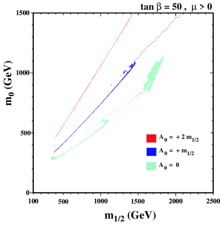
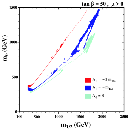
Figure 2: The WMAP strips for $\mu>0$, $m_{t}=178\,\,\mathrm{GeV}$ and (a) $\tan\beta=10$, $A_{0}\geq 0$ (upper left), (b) $\tan\beta=10$, $A_{0}\leq 0$ (upper right), (c) $\tan\beta=50$, $A_{0}\geq 0$ (lower left), (d) $\tan\beta=50$, $A_{0}\leq 0$ (lower right) showing the dependence on $A_{0}$ for $A_{0}=0,\pm m_{1/2}$ and $\pm 2m_{1/2}$.

The WMAP regions for $\tan\beta=50$ vary much more rapidly with $|A_{0}|$, because of the sensitivity of the $A,H$ masses and hence the rapid-annihilation regions. In Fig. 2(c) the case for $A_{0}\geq 0$ can be seen, whereas Fig. 2(d) shows $A_{0}\leq 0$. We again see wisps of allowed CMSSM parameter space due to rapid $\tilde{\tau}_{1}\bar{\tilde{\tau}}_{1}\to H$ annihilation. In this case, as described above, the right-handed stau mass is sensitive to the value of $A_{0}$. Therefore, for $A_{0}\neq 0$ (Fig. 2(c,d)), the cosmologically preferred region shifts to larger $m_{0}$ for both signs of $A_{0}$. In addition, the value of the heavy Higgs scalar and pseudoscalar masses depends on $A_{0}$ (not only $A_{0}^{2}$) and the position of the rapid-annihilation funnels therefore depends sensitively on $A_{0}$.

In the following, we mainly present our results along the WMAP strips for $m_{t}=178\,\,\mathrm{GeV}$, the present experimental central value [21], but we do show results for different values of $|A_{0}|$. This is because the variation with $m_{t}$ is less important for $\tan\beta=10$, and comparable with that due to varying $|A_{0}|$ when $\tan\beta=50$. Additionally, we present scans of the $(m_{1/2},A_{0})$ planes for $\tan\beta=10$ and 50.

3 Present and future sensitivities to the scale of supersymmetry from low-energy observables

In this section, we briefly describe the low-energy observables used in our analysis. We discuss the current and prospective future precision of the experimental results and the theoretical predictions. In the following, we refer to the theoretical uncertainties from unknown higher-order corrections as ‘intrinsic’ theoretical uncertainties and to the uncertainties induced by the experimental errors of the input parameters as ‘parametric’ theoretical uncertainties. We also give relevant details of the higher-order perturbative corrections that we include. We do not discuss theoretical uncertainties from the RG running between the high-scale parameters and the weak scale (see Ref. [19] for a recent discussion in the context of predicting the CDM density). At present, these uncertainties are expected to be less important than the experimental and theoretical uncertainties of the precision observables. In the future, both the uncertainties from unknown higher-order terms in the RG running and from the parameters entering the running will considerably improve.

Results for these observables are shown as a function of $m_{1/2}$ with $A_{0}$ varied, $m_{0}$ determined by the WMAP constraint (see Sect. 2), and $\tan\beta=10,50$. In this way the indirect sensitivities of the low-energy observables to the scale of supersymmetry are investigated.

3.1 The $W$ boson mass

The $W$ boson mass can be evaluated from

$$M_{W}^{2}\left(1-\frac{M_{W}^{2}}{M_{Z}^{2}}\right)=\frac{\pi\alpha}{\sqrt{2}G_{F}}\left(1+\Delta r\right),$$ (1)

where $\alpha$ is the fine structure constant and $G_{F}$ the Fermi constant. The radiative corrections are summarized in the quantity $\Delta r$ [24]. The prediction for $M_{W}$ within the Standard Model (SM) or the MSSM is obtained from evaluating $\Delta r$ in these models and solving eq. (1) in an iterative way.

The one-loop contributions to $\Delta r$ can be written as

$$\Delta r=\Delta\alpha-\frac{c_{W}^{2}}{s_{W}^{2}}\Delta\rho+(\Delta r)_{\rm rem},$$ (2)

where $\Delta\alpha$ is the shift in the fine structure constant due to the light fermions of the SM, $\Delta\alpha\propto\log m_{f}$, and $\Delta\rho$ is the leading contribution to the $\rho$ parameter. It is given by fermion and sfermion loop contributions to the transverse parts of the gauge boson self-energies at zero external momentum,

$$\Delta\rho=\frac{\Sigma_{Z}(0)}{M_{Z}^{2}}-\frac{\Sigma_{W}(0)}{M_{W}^{2}}~{}.$$ (3)

The remainder part, $(\Delta r)_{\rm rem}$, contains in particular the contributions from the Higgs sector.

We include the complete one-loop result in the MSSM [25, 26] as well as higher-order QCD corrections of SM type of ${\cal O}(\alpha\alpha_{s})$ [27, 28] and ${\cal O}(\alpha\alpha_{s}^{2})$ [29, 30]. Furthermore, we incorporate supersymmetric corrections of ${\cal O}(\alpha\alpha_{s})$ [31] and of ${\cal O}(\alpha_{t}^{2})$ [32] to $\Delta\rho$.

The remaining intrinsic theoretical uncertainty in the prediction for $M_{W}$ within the MSSM is still significantly larger than in the SM, where it is currently estimated to be about 4 MeV [33]. We estimate the present [34] and future intrinsic uncertainties to be

$$\Delta M_{W}^{\rm intr,current}=10\,\,\mathrm{MeV},\quad\Delta M_{W}^{\rm intr,future}=2\,\,\mathrm{MeV}.$$ (4)

The parametric uncertainties are dominated by the experimental error of the top-quark mass and the hadronic contribution to the shift in the fine structure constant. The current errors induce the following parametric uncertainties

$$\delta m_{t}^{\rm current}=4.3\,\,\mathrm{GeV} \Rightarrow \Delta M_{W}^{{\rm para},m_{t},{\rm current}}\approx 26\,\,\mathrm{MeV},$$ (5)

$$\delta(\Delta\alpha_{\rm had}^{\rm current})=36\times 10^{-5} \Rightarrow \Delta M_{W}^{{\rm para},\Delta\alpha_{\rm had},{\rm current}}\approx 6.5\,\,\mathrm{MeV}.$$ (6)

At the ILC, the top-quark mass will be measured with an accuracy of about 100 MeV [2]. The parametric uncertainties induced by the future experimental errors of $m_{t}$ and $\Delta\alpha_{\rm had}$ [35] will then be [36]

$$\delta m_{t}^{\rm future}=0.1\,\,\mathrm{GeV} \Rightarrow \Delta M_{W}^{{\rm para},m_{t},{\rm future}}\approx 1\,\,\mathrm{MeV},$$ (7)

$$\delta(\Delta\alpha_{\rm had}^{\rm future})=5\times 10^{-5} \Rightarrow \Delta M_{W}^{{\rm para},\Delta\alpha_{\rm had},{\rm future}}\approx 1\,\,\mathrm{MeV}.$$ (8)

The present experimental value of $M_{W}$ is [1]

$$M_{W}^{\rm exp,current}=80.425\pm 0.034~{}{\rm GeV}.$$ (9)

With the GigaZ option of the ILC (i.e. high-luminosity running at the $Z$ resonance and the $WW$ threshold) the $W$-boson mass will be determined with an accuracy of about [37, 38]

$$\delta M_{W}^{\rm exp,future}=7\,\,\mathrm{MeV}.$$ (10)

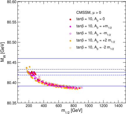
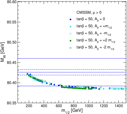
Figure 3: The CMSSM prediction for $M_{W}$ as a function of $m_{1/2}$ along the WMAP strips for (a) $\tan\beta=10$ and (b) $\tan\beta=50$ for various $A_{0}$ values. In each panel, the centre (solid) line is the present central experimental value, and the (solid) outer lines show the current $\pm 1$-$\sigma$ range. The dashed lines correspond to the anticipated GigaZ accuracy, assuming the same central value.

In all plots of this section we show the theory predictions without parametric and intrinsic theoretical uncertainties (using $m_{t}=178$ GeV). In the fits carried out in Sects. 4 and 5 below we take both parametric and intrinsic theoretical uncertainties into account.

We display in Fig. 3 the CMSSM prediction for $M_{W}$ and compare it with the present measurement (solid lines) and a possible future determination with GigaZ (dashed lines). Panel (a) shows the values of $M_{W}$ obtained with $\tan\beta=10$ and $|A_{0}|\leq 2$, and panel (b) shows the same for $\tan\beta=50$. It is striking that the present central value of $M_{W}$ (for both values of $\tan\beta$) favours low values of $m_{1/2}\sim 200$–$300$ GeV, though values as large as 800 GeV are allowed at the 1-$\sigma$ level, and essentially all values of $m_{1/2}$ are allowed at the $90\%$ confidence level. The GigaZ determination of $M_{W}$ might be able to determine indirectly a low value of $m_{1/2}$ with an accuracy of $\pm 50\,\,\mathrm{GeV}$, but even the GigaZ precision would still be insufficient to determine $m_{1/2}$ accurately if $m_{1/2}\;\raisebox{-3.00003pt}{$\stackrel{{\scriptstyle\displaystyle>}}{{\sim}}$}\;600\,\,\mathrm{GeV}$.

3.2 The effective leptonic weak mixing angle

The effective leptonic weak mixing angle at the $Z$ boson resonance can be written as

$$\sin^{2}\theta_{\mathrm{eff}}=\frac{1}{4}\,\left(1-\mbox{Re}\,\frac{v_{\rm eff}}{a_{\rm eff}}\right)\ ,$$ (11)

where $v_{\rm eff}$ and $a_{\rm eff}$ denote the effective vector and axial couplings of the $Z$ boson to charged leptons. As in the case of $M_{W}$, the leading supersymmetric higher-order corrections enter via the $\rho$ parameter,

$$\delta\sin^{2}\theta_{\mathrm{eff}}\approx-\frac{c_{W}^{2}s_{W}^{2}}{c_{W}^{2}-s_{W}^{2}}\Delta\rho.$$ (12)

Our theoretical prediction for $\sin^{2}\theta_{\mathrm{eff}}$ contains the same higher-order corrections as described in Sect. 3.1.

In the SM, the remaining intrinsic theoretical uncertainty in the prediction for $\sin^{2}\theta_{\mathrm{eff}}$ has been estimated to be about $5\times 10^{-5}$ [39]. For the MSSM, we use as present [34] and future intrinsic uncertainties

$$\Delta\sin^{2}\theta_{\mathrm{eff}}^{\rm intr,current}=12\times 10^{-5},\quad\Delta\sin^{2}\theta_{\mathrm{eff}}^{\rm intr,future}=2\times 10^{-5}.$$ (13)

The current experimental errors of $m_{t}$ and $\Delta\alpha_{\rm had}$ induce the following parametric uncertainties

$$\delta m_{t}^{\rm current}=4.3\,\,\mathrm{GeV} \Rightarrow \Delta\sin^{2}\theta_{\mathrm{eff}}^{{\rm para},m_{t},{\rm current}}\approx 14\times 10^{-5},$$ (14)

$$\delta(\Delta\alpha_{\rm had}^{\rm current})=36\times 10^{-5} \Rightarrow \Delta\sin^{2}\theta_{\mathrm{eff}}^{{\rm para},\Delta\alpha_{\rm had},{\rm current}}\approx 13\times 10^{-5}.$$ (15)

These should improve in the future to

$$\delta m_{t}^{\rm future}=0.1\,\,\mathrm{GeV} \Rightarrow \Delta\sin^{2}\theta_{\mathrm{eff}}^{{\rm para},m_{t},{\rm future}}\approx 0.4\times 10^{-5},$$ (16)

$$\delta(\Delta\alpha_{\rm had}^{\rm future})=5\times 10^{-5} \Rightarrow \Delta\sin^{2}\theta_{\mathrm{eff}}^{{\rm para},\Delta\alpha_{\rm had},{\rm future}}\approx 1.8\times 10^{-5}.$$ (17)

It is well known that there is a 2.8-$\sigma$ discrepancy [1] between the leptonic and heavy-flavour determinations of the electroweak mixing angle, with the leptonic measurement of $\sin^{2}\theta_{\mathrm{eff}}$ tending to pull down the value of Higgs-boson mass preferred in the SM fit, whereas the heavy-flavour measurements favour a larger value of the Higgs mass. The Electroweak Working Group notes that the overall quality of a global electroweak fit is quite acceptable, $\sim 26\%$ [1], and we use their combination of the two sets of measurements:

$$\sin^{2}\theta_{\mathrm{eff}}^{\rm exp,current}=0.23150\pm 0.00016.$$ (18)

The experimental accuracy will improve to about

$$\delta\sin^{2}\theta_{\mathrm{eff}}^{\rm exp,future}=1\times 10^{-5}.$$ (19)

at GigaZ [40].

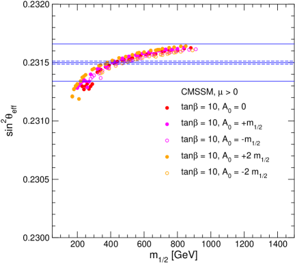
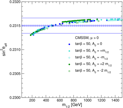
Figure 4: The CMSSM prediction for $\sin^{2}\theta_{\mathrm{eff}}$ as a function of $m_{1/2}$ along the WMAP strips for (a) $\tan\beta=10$ and (b) $\tan\beta=50$ for various $A_{0}$ values. In each panel, the centre (solid) line is the present central experimental value, and the (solid) outer lines show the current $\pm 1$-$\sigma$ range. The dashed lines correspond to the anticipated GigaZ accuracy, assuming the same central value.

Fig. 4 shows the prediction for $\sin^{2}\theta_{\mathrm{eff}}$ in the CMSSM compared with the present and future experimental precision. As in the case of $M_{W}$, low values of $m_{1/2}$ are also favoured independently by $\sin^{2}\theta_{\mathrm{eff}}$. The present central value prefers $m_{1/2}=300$–$500\,\,\mathrm{GeV}$, but the 1-$\sigma$ range extends beyond 1500 GeV (depending on $A_{0}$), and all values of $m_{1/2}$ are allowed at the $90\%$ confidence level. The GigaZ precision on $\sin^{2}\theta_{\mathrm{eff}}$ would be able to determine $m_{1/2}$ indirectly with even greater accuracy than $M_{W}$ at low $m_{1/2}$, but would also be insufficient if $m_{1/2}\;\raisebox{-3.00003pt}{$\stackrel{{\scriptstyle\displaystyle>}}{{\sim}}$}\;700\,\,\mathrm{GeV}$.

3.3 The anomalous magnetic moment of the muon

We now discuss the evaluation of the MSSM contributions to the anomalous magnetic moment of the muon, $a_{\mu}\equiv(g-2)_{\mu}$. Since the possible deviation of the SM prediction from the experimental result is crucial for the interpretation of the $a_{\mu}$ results, we first review this aspect in the light of recent developments.

The SM prediction for the anomalous magnetic moment of the muon (see Refs. [41, 42] for reviews) depends on the evaluation of the hadronic vacuum polarization and light-by-light (LBL) contributions. The former have been evaluated in [43, 44, 45, 46] and the latter in [47, 48]. The evaluations of the hadronic vacuum polarization contributions using $e^{+}e^{-}$ and $\tau$ decay data give somewhat different results. Recently, new data have been published by the KLOE Collaboration [49], which agree well with the previous data from CMD-2. This, coupled with a greater respect for the uncertainties inherent in the isospin transformation from $\tau$ decay, has led to a proposal to use the $e^{+}e^{-}$ alone and shelve the $\tau$ data, resulting in the estimate [50]

$$a_{\mu}^{\rm theo}=(11\,659\,182.8\pm 6.3_{\rm had}\pm 3.5_{\rm LBL}\pm 0.3_{\rm QED+EW})\times 10^{-10},$$ (20)

where the source of each error is labelled .

This result is to be compared with the final result of the Brookhaven $(g-2)_{\mu}$ Experiment E821, namely [52]

$$a_{\mu}^{\rm exp}=(11\,659\,208.0\pm 5.8)\times 10^{-10},$$ (21)

leading to an estimated discrepancy

$$a_{\mu}^{\rm exp}-a_{\mu}^{\rm theo}=(25.2\pm 9.2)\times 10^{-10},$$ (22)

equivalent to a 2.7 $\sigma$ effect. In view of the chequered history of the SM prediction, eq. (20), and the residual questions concerning the use of the $\tau$ decay data, it would be premature to regard this discrepancy as firm evidence of new physics. We do note, on the other hand, that the $(g-2)_{\mu}$ measurement imposes an important constraint on supersymmetry, even if one uses the $\tau$ decay data. We use eq. (22) for our numerical discussion below.

The following MSSM contributions to the theoretical prediction for $a_{\mu}$ have been considered. We take fully into account the complete one-loop contribution to $a_{\mu}$, which was evaluated nearly a decade ago in Ref. [53]. We make no simplification in the sparticle mass scales but, for illustrating the possible size of corrections, a simplified formula can be used, in which relevant supersymmetric mass scales are set to a common value, $M_{\rm SUSY}=m_{\tilde{\chi}^{\pm}}=m_{\tilde{\chi}^{0}}=m_{\tilde{\mu}}=m_{\tilde{\nu}_{\mu}}$. The result in this approximation is given by

$$a_{\mu}^{\mathrm{SUSY},{\rm 1L}}=13\times 10^{-10}\left(\frac{100\,\,\mathrm{GeV}}{M_{\rm SUSY}}\right)^{2}\tan\beta\;{\rm sign}(\mu).$$ (23)

We see that supersymmetric effects can easily account for a $(20\ldots 30)\times 10^{-10}$ deviation, if $\mu$ is positive and $M_{\rm SUSY}$ lies roughly between 100 GeV (for small $\tan\beta$) and 600 GeV (for large $\tan\beta$). For this reason, in the rest of this paper, we restrict our attention to $\mu>0$. Even in view of the possible size of experimental and theoretical uncertainties, it is very difficult to reconcile $\mu<0$ with the present data on $a_{\mu}$.

In addition to the full one-loop contributions, we also include several two-loop corrections. The first class of corrections comprises the leading $\log\left(m_{\mu}/M_{\rm SUSY}\right)$ terms of supersymmetric one-loop diagrams with a photon in the second loop, which are given by [54]:

$$\Delta a_{\mu}^{\mathrm{SUSY},{\rm 2L,QED}}=\Delta a_{\mu}^{\rm SUSY,1L}\times\left(\frac{4\,\alpha}{\pi}\log\left(\frac{M_{\rm SUSY}}{m_{\mu}}\right)\right)~{}.$$ (24)

These amount to about $-8\%$ of the supersymmetric one-loop contribution for a supersymmetric mass scale $M_{\rm SUSY}=500\,\,\mathrm{GeV}$.

The second class of two-loop corrections comprises diagrams with a closed loop of SM fermions or scalar fermions. These were calculated in Ref. [55], where it was demonstrated that these corrections may amount to $\sim 5\times 10^{-10}$ in the general MSSM, if all experimental bounds are taken into account. These corrections are included in the Fortran code FeynHiggs [56, 57]. We have furthermore taken into account the 2-loop contributions to $a_{\mu}$ from diagrams containing a closed chargino/neutralino loop, which have been evaluated in [58]. Here we use an approximate form for these corrections, which are typically $\sim 1\times 10^{-10}$.

The current intrinsic uncertainties in the MSSM contributions to $a_{\mu}$ can be estimated to be $\sim 6\times 10^{-10}$ [58, 59]. In the more restricted CMSSM parameter space the intrinsic uncertainties are smaller, being about $1\times 10^{-10}$. Once the full two-loop result in the MSSM is available, this uncertainty will be further reduced. We assume that in the future the uncertainty in eq. (22) will be reduced by a factor two.

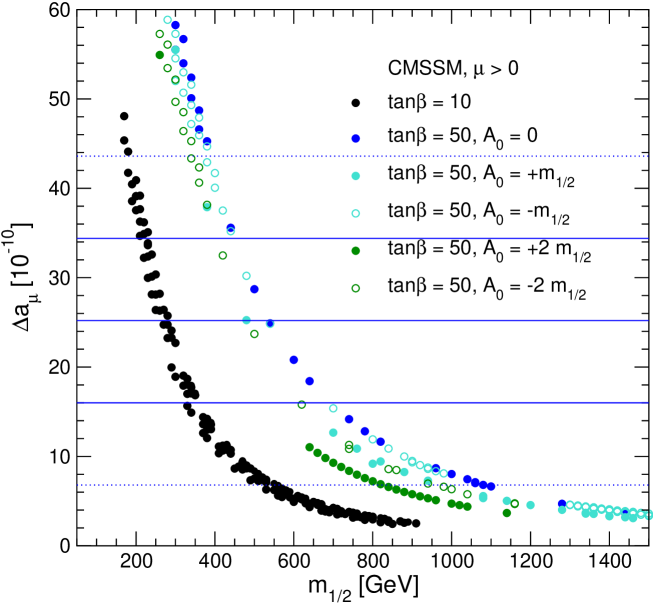
Figure 5: The CMSSM prediction for $\Delta a_{\mu}$ as a function of $m_{1/2}$ along the WMAP strips for $\tan\beta=10,50$ and different $A_{0}$ values. The central (solid) line is the central value of the present discrepancy between experiment and the SM value evaluated using $e^{+}e^{-}$ data (see text), and the other solid (dotted) lines show the current $\pm 1(2)$-$\sigma$ ranges, eq. (22).

As seen in Fig. 5, the CMSSM prediction for $a_{\mu}$ is almost independent of $A_{0}$ for $\tan\beta=10$, but substantial variations are possible for $\tan\beta=50$, except at very large $m_{1/2}$. In the case $\tan\beta=10$, $m_{1/2}\sim 200$–400 GeV is again favoured at the $\pm 1$-$\sigma$ level, but this preferred range shifts up to 400 to 800 GeV if $\tan\beta=50$, depending on the value of $A_{0}$. At the 2-$\sigma$ level, there is nominally an upper bound $m_{1/2}\;\raisebox{-3.00003pt}{$\stackrel{{\scriptstyle\displaystyle<}}{{\sim}}$}\;600(1100)\,\,\mathrm{GeV}$ for $\tan\beta=10(50)$, but according to the discussion above it should be interpreted with care. Nevertheless, the lower bound to $m_{1/2}$ for both $\tan\beta=10$ and 50 should be regarded as relatively robust. On the other hand, it is striking that $M_{W}$, $\sin^{2}\theta_{\mathrm{eff}}$ and $a_{\mu}$ all favour small $m_{1/2}$ for $\tan\beta=10$. If $\tan\beta=50$, the consistency between the ranges preferred by the different observables is not so striking.

3.4 The decay $b\to s\gamma$

Since this decay occurs at the loop level in the SM, the MSSM contribution might, a priori, be of similar magnitude. The most up-to-date theoretical estimate of the SM contribution to the branching ratio is [60]

$${\rm BR}(b\to s\gamma)=(3.70\pm 0.30)\times 10^{-4},$$ (25)

where the calculations have been carried out completely to NLO in the $\overline{\rm{MS}}$ renormalization scheme, and the error is dominated by higher-order QCD uncertainties. A complete NNLO QCD calculation is now underway, and will reduce significantly the uncertainty, once it is available.

For comparison, the present experimental value estimated by the Heavy Flavour Averaging Group (HFAG) is [61]

$${\rm BR}(b\to s\gamma)=(3.54^{+0.30}_{-0.28})\times 10^{-4},$$ (26)

where the error includes an uncertainty due to the decay spectrum, as well as the statistical error. The very good agreement between eq. (26) and the SM calculation eq. (25) imposes important constraints on the MSSM, as we see below.

Our numerical results have been derived and checked with three different codes. The first is based on Refs. [62, 63] and the second is based on Refs. [63, 64]. Results have been derived using the charm pole mass as well as the charm running mass, giving an estimate of remaining higher-order uncertainties. Finally, our results have been checked with the ${\rm BR}(b\to s\gamma)$ evaluation provided in Ref. [65], which yielded very similar results to our two other approaches. For the current theoretical uncertainty of the MSSM prediction for ${\rm BR}(b\to s\gamma)$ we use the value of eq. (25). For the future uncertainty from the experimental as well as the theoretical side we assume a reduction by a factor of 3.

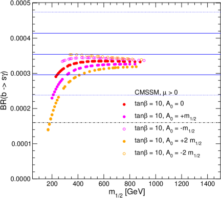
Figure 6: The CMSSM predictions for ${\rm BR}(b\to s\gamma)$ as a function of $m_{1/2}$ along the WMAP strips for (a) $\tan\beta=10$ and (b) $\tan\beta=50$ and various choices of $A_{0}$. The uncertainty shown combines linearly the current experimental error and the present theoretical uncertainty in the SM prediction. The central (solid) line indicates the current experimental central value, and the other solid (dotted) lines show the current $\pm 1(2)$-$\sigma$ ranges. The dash-dotted line corresponds to a more conservative estimate of intrinsic uncertainties (see text).

As already mentioned, the present central value of this branching ratio agrees very well with the SM, implying that large values of $m_{1/2}$ cannot be excluded for any value of $\tan\beta$. The uncertainty range shown in Fig. 6 combines linearly the current experimental error and the present theoretical uncertainty in the SM prediction. Note however, that at present there is also an uncertainty in the computed MSSM value (included in obtaining the excluded regions in Figs. 1 and 2) from the uncertainty in the SUSY loop calculations. Taking this conservatively into account results in a 95% C.L. exclusion bound of 0.00016 in the case of $\tan\beta=10$, and of 0.000195 in the case of $\tan\beta=50$. These values are shown as dash-dotted lines in Fig. 6. This allows a somewhat lower range in $m_{1/2}$ than depicted in Fig. 6. We assume that these uncertainties can be significantly reduced in the future. We have checked that they have no significant impact on the results presented below.

Since the CMSSM corrections are generally smaller for smaller $\tan\beta$, even values of $m_{1/2}$ as low as $\sim 200\,\,\mathrm{GeV}$ would be allowed at the $90\%$ confidence level if $\tan\beta=10$, whereas $m_{1/2}\;\raisebox{-3.00003pt}{$\stackrel{{\scriptstyle\displaystyle>}}{{\sim}}$}\;450\,\,\mathrm{GeV}$ would be required if $\tan\beta=50$. These limits are very sensitive to $A_{0}$, and, if the future error in ${\rm BR}(b\to s\gamma)$ could indeed be reduced by a factor $\sim 3$, the combination of ${\rm BR}(b\to s\gamma)$ with the other precision observables might be able, in principle, to constrain $A_{0}$ significantly.

3.5 The branching ratio $B_{s}\to\mu^{+}\mu^{-}$

The SM prediction for this branching ratio is $(3.4\pm 0.5)\times 10^{-9}$ [66], and the present experimental upper limit from the Fermilab Tevatron collider is $3.4\times 10^{-7}$ at the $95\%$ C.L. [67], providing ample room for the MSSM to dominate the SM contribution. The current Tevatron sensitivity, being based on an integrated luminosity of about 410 $\mbox{pb}^{-1}$ summed over both detectors, is expected to improve significantly in the future. A naive scaling of the present bound with the square root of the luminosity yields a sensitivity at the end of Run II of about $5.4\times 10^{-8}$ assuming 8 $\mbox{fb}^{-1}$ collected with each detector. An even bigger improvement may be possible with better signal acceptance and more efficient background reduction. In Ref. [68] an estimate of the future Tevatron sensitivity of $2\times 10^{-8}$ at the 90% C.L. has been given, and a sensitivity even down to the SM value can be expected at the LHC. Assuming the SM value, i.e. ${\rm BR}(B_{s}\to\mu^{+}\mu^{-})\approx 3.4\times 10^{-9}$, it has been estimated [69] that LHCb can observe 33 signal events over 10 background events within 3 years of low-luminosity running. Therefore this process offers good prospects for probing the MSSM.

For the theoretical prediction we use results from Ref. [70], which include the full one-loop evaluation and the leading two-loop QCD corrections. We are not aware of a detailed estimate of the theoretical uncertainties from unknown higher-order corrections.

Figure 7: The CMSSM prediction for ${\rm BR}(B_{s}\to\mu^{+}\mu^{-})$ as a function of $m_{1/2}$ along the WMAP strips for $\tan\beta=10$ and all $A_{0}$ values, and for $\tan\beta=50$ with various values of $A_{0}$. The solid line shows the current Tevatron limit at the 95% C.L., and the dotted line corresponds to an estimate for the sensitivity of the Tevatron at the end of Run II.

In Fig. 7 the CMSSM prediction for ${\rm BR}(B_{s}\to\mu^{+}\mu^{-})$ as a function of $m_{1/2}$ is compared with the present Tevatron limit and our estimate for the sensitivity at the end of Run II. For $\tan\beta=10$ the CMSSM prediction is significantly below the present and future Tevatron sensitivity. With the current sensitivity, the Tevatron starts to probe the CMSSM region with $\tan\beta=50$. The sensitivity at the end of Run II will test the CMSSM parameter space with $\tan\beta=50$ and $m_{1/2}\;\raisebox{-3.00003pt}{$\stackrel{{\scriptstyle\displaystyle<}}{{\sim}}$}\;600\,\,\mathrm{GeV}$, in particular for positive values of $A_{0}$. The LHC will be able to probe the whole CMSSM parameter space via this rare decay.

3.6 The lightest MSSM Higgs boson mass

The mass of the lightest ${\cal CP}$-even MSSM Higgs boson can be predicted in terms of the other CMSSM parameters. At the tree level, the two ${\cal CP}$-even Higgs boson masses are obtained as a function of $M_{Z}$, the ${\cal CP}$-odd Higgs boson mass $M_{A}$, and $\tan\beta$. In the Feynman-diagrammatic (FD) approach, which we employ here, the higher-order corrected Higgs boson masses are derived by finding the poles of the $h,H$-propagator matrix. This is equivalent to solving

$$\left[p^{2}-m_{h,\rm tree}^{2}+\hat{\Sigma}_{hh}(p^{2})\right]\times\left[p^{2}-m_{H,\rm tree}^{2}+\hat{\Sigma}_{HH}(p^{2})\right]-\left[\hat{\Sigma}_{hH}(p^{2})\right]^{2}=0~{},$$ (27)

where the $\hat{\Sigma}(p^{2})$ denote the renormalized Higgs-boson self-energies, and $p$ is the external momentum.

For the theoretical prediction of $M_{h}$ we use the code FeynHiggs [56, 57], which includes all numerically relevant known higher-order corrections. The status of the incorporated results for the self-energy contributions to eq. (27) can be summarized as follows. For the one-loop part, the complete result within the MSSM is known [71, 72, 73]. Concerning the two-loop effects, their computation is quite advanced, see Ref. [74] and references therein. They include the strong corrections at ${\cal O}(\alpha_{t}\alpha_{s})$ and Yukawa corrections at ${\cal O}(\alpha_{t}^{2})$, as well as the dominant one-loop ${\cal O}(\alpha_{t})$ term, and the strong corrections from the bottom/sbottom sector at ${\cal O}(\alpha_{b}\alpha_{s})$. For the $b/\tilde{b}$ sector corrections also an all-order resummation of the $\tan\beta\hskip 2.84526pt$-enhanced terms, ${\cal O}(\alpha_{b}(\alpha_{s}\tan\beta)^{n})$, is known [75, 76]. Most recently, the ${\cal O}(\alpha_{t}\alpha_{b})$ and ${\cal O}(\alpha_{b}^{2})$ corrections have been derived [77].

The current intrinsic error of $M_{h}$ due to unknown higher-order corrections and its prospective improvement in the future have been estimated to be [74, 79]

$$\Delta M_{h}^{\rm intr,current}=3\,\,\mathrm{GeV},\quad\Delta M_{h}^{\rm intr,future}=0.5\,\,\mathrm{GeV}.$$ (28)

The estimated future uncertainty assumes that a full two-loop result, leading three-loop and possibly even higher-order corrections become available.

Concerning the parametric error on $M_{h}$, the top-quark mass has the largest impact, entering $\propto m_{t}^{4}$ at the one-loop level. As a rule of thumb, an uncertainty of $\delta m_{t}=1\,\,\mathrm{GeV}$ translates to an induced parametric uncertainty in $M_{h}$ of $\Delta M_{h}^{m_{t}}\approx 1\,\,\mathrm{GeV}$ [80]. We find for the parametric uncertainties induced by the present experimental errors of $m_{t}$ and $\alpha_{s}$

$$\delta m_{t}^{\rm current}=4.3\,\,\mathrm{GeV} \Rightarrow \Delta M_{h}^{{\rm para},m_{t},{\rm current}}\approx 4\,\,\mathrm{GeV},$$ (29)

$$\delta\alpha_{s}^{\rm current}=0.002 \Rightarrow \Delta M_{h}^{{\rm para},\alpha_{s},{\rm current}}\approx 0.3\,\,\mathrm{GeV}.$$ (30)

These will improve in the future to

$$\delta m_{t}^{\rm future}=0.1\,\,\mathrm{GeV} \Rightarrow \Delta M_{h}^{{\rm para},m_{t},{\rm future}}\approx 0.1\,\,\mathrm{GeV},$$ (31)

$$\delta\alpha_{s}^{\rm future}=0.001 \Rightarrow \Delta M_{h}^{{\rm para},\alpha_{s},{\rm future}}\approx 0.1\,\,\mathrm{GeV}.$$ (32)

Thus, the intrinsic error would be the dominant source of uncertainty in the future. On the other hand, a further reduction of the unknown higher-order corrections to $M_{h}$ is in principle possible.

Figure 8: The CMSSM predictions for $M_{h}$ as functions of $m_{1/2}$ with (a) $\tan\beta=10$ and (b) $\tan\beta=50$ for various $A_{0}$. A hypothetical experimental value is shown, namely $M_{h}=120\,\,\mathrm{GeV}$. We display an optimistic anticipated theory uncertainty of $\pm 0.2\,\,\mathrm{GeV}$, as well as a more realistic theory uncertainty of $\pm 0.5\,\,\mathrm{GeV}$ and the current theory uncertainty of $\pm 3\,\,\mathrm{GeV}$.

The experimental accuracy on $M_{h}$ at the ILC [2] will be even higher than the prospective precision of the theory prediction,

$$\delta M_{h}^{\rm exp,future}=0.05\,\,\mathrm{GeV}.$$ (33)

We show in Fig. 8 we show the for $M_{h}$, assuming a hypothetical measurement at $M_{h}=120\,\,\mathrm{GeV}$. Since the experimental error at the ILC will be smaller than the prospective theory uncertainties, we display the effect of the current and future intrinsic uncertainties. In addition, a more optimistic value of 200 MeV is also shown. The figure clearly illustrates the high sensitivity of this electroweak precision observable to variations of the supersymmetric parameters (detailed results for Higgs boson phenomenology in the CMSSM can be found in Ref. [81]). The comparison between the measured value of $M_{h}$ and a precise theory prediction will allow one to set tight constraints on the allowed parameter space of $m_{1/2}$ and $A_{0}$.

3.7 The Higgs boson branching ratios

Within the CMSSM, various Higgs boson decay channels will be accessible at the LHC and the ILC. At the LHC, Higgs boson couplings [82] or ratios of them [83, 84] can in general be determined at the level of $\sim 10\%$ at best, depending on the Higgs-boson mass and theoretical assumptions. Therefore we concentrate on ILC measurements and accuracies.

It has been shown in Ref. [85] that the observable combination

$$r\equiv\frac{\left[{\rm BR}(h\to b\bar{b})/{\rm BR}(h\to WW^{*})\right]_{\rm MSSM}}{\left[{\rm BR}(h\to b\bar{b})/{\rm BR}(h\to WW^{*})\right]_{\rm SM~{}~{}~{}}\,}$$ (34)

of Higgs boson decay rates is particularly sensitive to deviations of the MSSM Higgs sector from the SM. Even though the experimental error on the ratio of the two branching ratios is larger than that on the individual ones, the quantity $r$ has a stronger sensitivity to $M_{A}$ than any single branching ratio.

For the evaluation of ${\rm BR}(h\to b\bar{b})$, we use the results of Ref. [86], including the result of resumming the contributions of ${\cal O}((\alpha_{s}\tan\beta)^{n})$ [75, 76]. The evaluation of ${\rm BR}(h\to WW^{*})$ is based on an effective-coupling approach, taking into account off-shell effects. The corrections used for the effective-coupling calculation are the same as for the Higgs-boson mass calculation, including the full one-loop and leading and subleading two-loop contributions [56, 74]. The evaluation has been performed with FeynHiggs [56, 57].

For the prospective accuracy at the ILC, we consider two cases. At the ILC with $\sqrt{s}=500\,\,\mathrm{GeV}$ an accuracy of 4% seems to be feasible [2], whilst at $\sqrt{s}=1\,\,\mathrm{TeV}$ this accuracy could be improved to [87]

$$\left(\frac{\delta r}{r}\right)^{\rm exp,future}=1.5\%.$$ (35)

Since in this ratio of branching ratios many theoretical uncertainties cancel, we assume that the future theoretical error can be neglected. In the analysis in Sect. 5 we use the accuracy of eq. (35).

Figure 9: The CMSSM predictions for $[{\rm BR}(h\to b\bar{b})/{\rm BR}(h\to WW^{*})]_{\rm MSSM}/[{\rm BR}(h\to b\bar{b})/{\rm BR}(h\to WW^{*})]_{\rm SM}$ as functions of $m_{1/2}$ for (a) $\tan\beta=10$ and (b) $\tan\beta=50$ with various values of $A_{0}$. The central (solid) line corresponds to the SM expectation. The outer (dotted) and inner (solid) lines indicate an ILC measurement with 4% and 1.5% accuracy, respectively.

In Fig. 9 the results for $r$ are shown as functions of $m_{1/2}$ for $\tan\beta=10,50$. In the figure we indicate accuracies of both 4% and 1.5%. For low $\tan\beta$, the high ILC accuracy in $r$ will allow one to detect a deviation from the SM prediction for all CMSSM points. For large $\tan\beta$, the effects of the supersymmetric contributions to $r$ are in general smaller. Deviations up to $m_{1/2}\approx 1$ TeV could be visible, depending somewhat on $A_{0}$.

4 Combined Sensitivity: Present Situation

4.1 Best fits for WMAP strips at fixed $A_{0}$

We now investigate the combined sensitivity of the four low-energy observables for which experimental measurements exist at present, namely $M_{W}$, $\sin^{2}\theta_{\mathrm{eff}}$, $(g-2)_{\mu}$ and ${\rm BR}(b\to s\gamma)$. Since only an upper bound exists for ${\rm BR}(B_{s}\to\mu^{+}\mu^{-})$, we discuss it separately below. We begin with an analysis of the sensitivity to $m_{1/2}$ moving along the WMAP strips with fixed values of $A_{0}$ and $\tan\beta$. The experimental central values, the present experimental errors and theoretical uncertainties are as described in Sect. 3. The experimental uncertainties, the intrinsic errors from unknown higher-order corrections and the parametric uncertainties have been added quadratically, except for ${\rm BR}(b\to s\gamma)$, where they have been added linearly. Assuming that the four observables are uncorrelated, a $\chi^{2}$ fit has been performed with

$$\chi^{2}\equiv\sum_{n=1}^{N}\left(\frac{R_{n}^{\rm exp}-R_{n}^{\rm theo}}{\sigma_{n}}\right)^{2}~{}.$$ (36)

Here $R_{n}^{\rm exp}$ denotes the experimental central value of the $n$th observable, so that $N=4$ for the set of observables included in this fit, $R_{n}^{\rm theo}$ is the corresponding CMSSM prediction and $\sigma_{n}$ denotes the combined error, as specified above. We have rejected all points of the CMSSM parameter space with either $M_{h}<113\,\,\mathrm{GeV}$ [88, 89] or a chargino mass lighter than $103\,\,\mathrm{GeV}$ [90].

Figure 10: The results of $\chi^{2}$ fits based on the current experimental results for the precision observables $M_{W}$, $\sin^{2}\theta_{\mathrm{eff}}$, $(g-2)_{\mu}$ and ${\rm BR}(b\to s\gamma)$ are shown as functions of $m_{1/2}$ in the CMSSM parameter space with CDM constraints for different values of $A_{0}$. The upper plot shows the results for $\tan\beta=10$, and the lower plot shows the case $\tan\beta=50$.

The results are shown in Fig. 10 for $\tan\beta=10$ and $\tan\beta=50$. They indicate that, already at the present level of experimental accuracies, the electroweak precision observables combined with the WMAP constraint provide a sensitive probe of the CMSSM, yielding interesting information about its parameter space. For $\tan\beta=10$, the CMSSM provides a very good description of the data, resulting in a remarkably small minimum $\chi^{2}$ value. The fit shows a clear preference for relatively small values of $m_{1/2}$, with a best-fit value of about $m_{1/2}=300\,\,\mathrm{GeV}$. The best fit is obtained for $A_{0}\leq 0$, while positive values of $A_{0}$ result in a somewhat lower fit quality. The fit yields an upper bound on $m_{1/2}$ of about 600 GeV at the 90% C.L. (corresponding to $\Delta\chi^{2}\leq 4.61$).

These results can easily be understood from the analysis in Sect. 3. For $\tan\beta=10$, the CMSSM prediction with $m_{1/2}\approx 300\,\,\mathrm{GeV}$ is very close to the experimental central values of $M_{W}$, $\sin^{2}\theta_{\mathrm{eff}}$ and $(g-2)_{\mu}$ for all values of $A_{0}$, see Figs. 3–5. Also, ${\rm BR}(b\to s\gamma)$ is well described for $m_{1/2}\approx 300\,\,\mathrm{GeV}$ and $A_{0}\leq 0$, while large positive values of $A_{0}$ lead to a CMSSM prediction for ${\rm BR}(b\to s\gamma)$ which is significantly below the experimental value. Consequently, in the case of $\tan\beta=10$, a very good fit quality is obtained for $m_{1/2}\approx 300\,\,\mathrm{GeV}$ and $A_{0}\leq 0$. Some of the principal contributions to the increase in $\chi^{2}$ when $m_{1/2}$ increases for $\tan\beta=10$ are as follows. For $A_{0}=-m_{1/2},m_{1/2}=900$ GeV, we find that $(g-2)_{\mu}$ contributes about 5 to $\Delta\chi^{2}$, $M_{W}$ nearly 1 and $\sin^{2}\theta_{\mathrm{eff}}$ about 0.2, whereas the contribution of ${\rm BR}(b\to s\gamma)$ is negligible. On the other hand, for $A_{0}=+2m_{1/2}$, which is disfavoured for $\tan\beta=10$, the minimum in $\chi^{2}$ is due to a combination of the four observables, but $(g-2)_{\mu}$ again gives the largest contribution for large $m_{1/2}$.

For $\tan\beta=50$ the overall fit quality is worse than for $\tan\beta=10$, and the sensitivity to $m_{1/2}$ from the precision observables is lower. This is related to the fact that, whereas $M_{W}$ and $\sin^{2}\theta_{\mathrm{eff}}$ prefer small values of $m_{1/2}$ also for $\tan\beta=50$, as seen in Figs. 3 and 4, the CMSSM predictions for $(g-2)_{\mu}$ and ${\rm BR}(b\to s\gamma)$ for high $\tan\beta$ are in better agreement with the data for larger $m_{1/2}$ values, as seen in Figs. 5 and 6. Also in this case the best fit is obtained for negative values of $A_{0}$, but the preferred values for $m_{1/2}$ are 200–300 GeV higher than for $\tan\beta=10$.

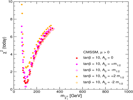
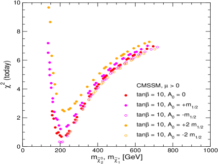
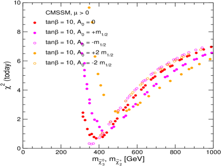
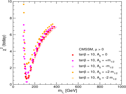
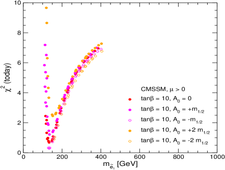
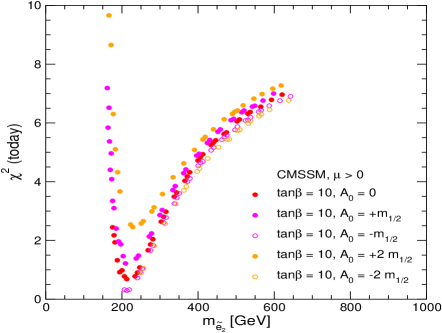
Figure 11: The $\chi^{2}$ contours in the CMSSM with $\tan\beta=10$ for different sparticle masses, based on the fits to the parameter space shown in Fig. 10. The first row shows (left) the mass of the neutralino LSP, $m_{\tilde{\chi}^{0}_{1}}$, and (right) the mass of the lighter chargino, $m_{\tilde{\chi}^{+}_{1}}\approx m_{\tilde{\chi}^{0}_{2}}$. The second row shows (left) the mass of the heavier chargino, $m_{\tilde{\chi}^{+}_{2}}\approx m_{\tilde{\chi}^{0}_{3}}$, and (right) the mass of the lighter stau, $m_{\tilde{\tau}_{1}}$. The selectron masses are shown in the third row.

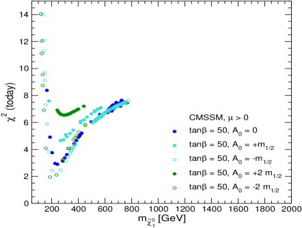
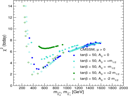
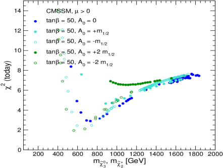
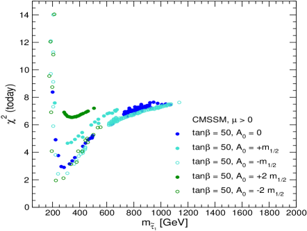
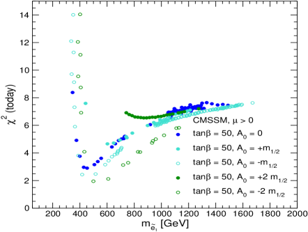
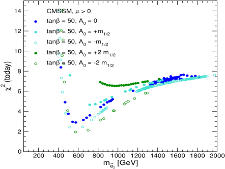
Figure 12: The $\chi^{2}$ contours in the CMSSM with $\tan\beta=50$ for different sparticle masses, based on the fits to the parameter space shown in Fig. 10. The first row shows (left) the mass of the lightest neutralino, $m_{\tilde{\chi}^{0}_{1}}$, and (right) the mass of the lighter chargino, $m_{\tilde{\chi}^{+}_{1}}\approx m_{\tilde{\chi}^{0}_{2}}$. The second row shows (left) the mass of the heavier chargino, $m_{\tilde{\chi}^{+}_{2}}\approx m_{\tilde{\chi}^{0}_{3}}$, and (right) the mass of the lighter stau, $m_{\tilde{\tau}_{1}}$. The selectron masses are shown in the third row.

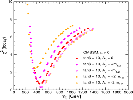
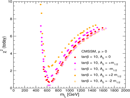
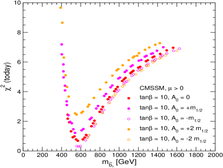
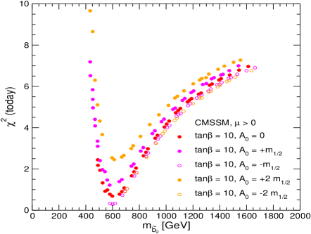
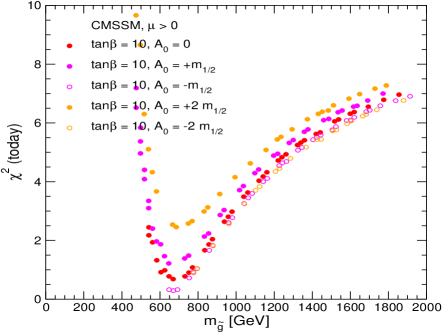
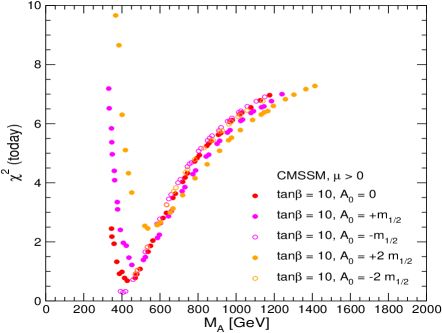
Figure 13: The $\chi^{2}$ contours in the CMSSM with $\tan\beta=10$ for different sparticle masses, based on the fits to the parameter space shown in Fig. 10. The first row shows the scalar top masses, $m_{\tilde{t}_{1}}$, $m_{\tilde{t}_{2}}$. The second row shows the scalar bottom masses, $m_{\tilde{b}_{1}}$, $m_{\tilde{b}_{2}}$. The third row shows the gluino mass, $m_{\tilde{g}}$, (left) and the mass of the scalar Higgs boson, $M_{A}$ (right).

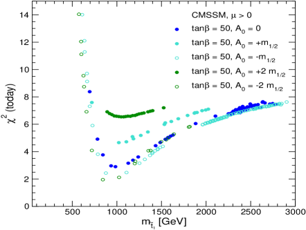
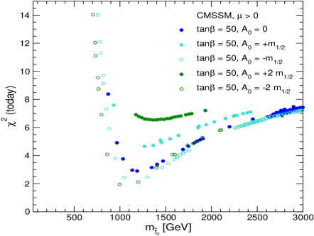
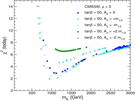
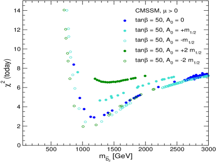
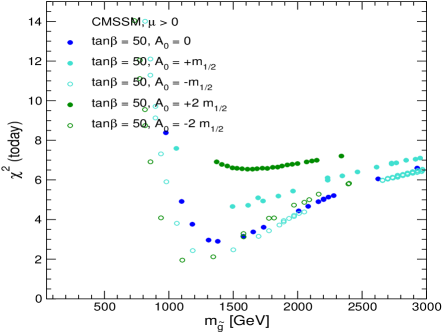
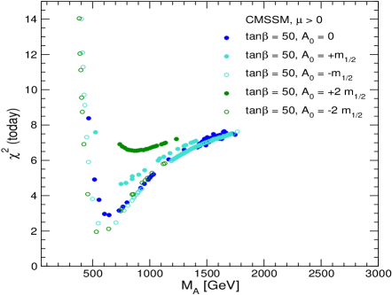
Figure 14: The $\chi^{2}$ contours in the CMSSM with $\tan\beta=50$ for different sparticle masses, based on the fits to the parameter space shown in Fig. 10. The first row shows the scalar top masses, $m_{\tilde{t}_{1}}$, $m_{\tilde{t}_{2}}$. The second row shows the scalar bottom masses, $m_{\tilde{b}_{1}}$, $m_{\tilde{b}_{2}}$. The third row shows the gluino mass, $m_{\tilde{g}}$, (left) and the mass of the scalar Higgs boson, $M_{A}$ (right).

In Figs. 11–14 the fit results of Fig. 10 are expressed in terms of the masses of different supersymmetric particles. Fig. 11 shows that for $\tan\beta=10$ the best fit is obtained if the lightest supersymmetric particle (LSP), which within the CMSSM is the lightest neutralino, is lighter than about 200 GeV (with a best-fit value $\sim 100$ GeV). The best-fit values for the masses of the lighter chargino, the second-lightest neutralino (recall also that $m_{\tilde{\chi}^{+}_{1}}\approx m_{\tilde{\chi}^{0}_{2}}$), both sleptons and the lighter stau are all below 250 GeV, while the preferred region of the masses of the heavier chargino and the heavier neutralinos is about 400 GeV. These masses offer good prospects of direct sparticle detection at both the ILC and the LHC. There are also some prospects for detecting the associated production of charginos and neutralinos at the Tevatron collider, via their trilepton decay signature, in particular. This is estimated to be sensitive to $m_{1/2}\mathrel{\hbox to0.0pt{\raise 2.15277pt\hbox{$<$}\hss}{\lower 2.15277pt\hbox{$\sim$}}}250$ GeV [91], covering much of the region below the best-fit value of $m_{1/2}$ that we find for $\tan\beta=10$.

The same particle masses in the case $\tan\beta=50$ are shown in Fig. 12. Here the best-fit values for the LSP mass and the lighter stau are still below about 250 GeV. The minimum $\chi^{2}$ for the other masses is shifted upwards compared to the case with $\tan\beta=10$. The best-fit values are obtained in the region 400–600 GeV. Correspondingly, these sparticles would be harder to detect. At the ILC with $\sqrt{s}\;\raisebox{-3.00003pt}{$\stackrel{{\scriptstyle\displaystyle<}}{{\sim}}$}\;1\,\,\mathrm{TeV}$, the best prospects would be for the production of $\tilde{\chi}^{0}_{1}\tilde{\chi}^{0}_{2}$ or of $\tilde{\tau}_{1}\bar{\tilde{\tau}}_{1}$. Other particles can only be produced if they turn out to be on the light side of the $\chi^{2}$ function.

In Fig. 13, 14 we focus on the coloured part of the supersymmetric spectrum and the Higgs mass scale. The case of $\tan\beta=10$ is shown in Fig. 13. The top row shows the two scalar top masses, the middle row displays the two scalar bottom masses, and the bottom row depicts the gluino mass and $M_{A}$. All the coloured particles should be accessible at the LHC. However, among them, only ${\tilde{t}}_{1}$ has a substantial part of its $\chi^{2}$-favoured spectrum below $500\,\,\mathrm{GeV}$, which would allow its detection at the ILC. The same applies for the mass of the $A$ boson. The Tevatron collider has a sensitivity to $m_{{\tilde{t}}_{1}}\mathrel{\hbox to0.0pt{\raise 2.15277pt\hbox{$<$}\hss}{\lower 2.15277pt\hbox{$\sim$}}}450$GeV, which is not far below our best-fit value for $\tan\beta=10$ [91].

Finally, in Fig. 14 we show the same masses in the case of $\tan\beta=50$. All the particles are mostly inaccessible at the ILC, though the LHC has good prospects. However, at the 90% C.L. the coloured sparticle masses might even exceed $\sim 3\,\,\mathrm{TeV}$, which would render their detection difficult. Concerning the heavy Higgs bosons, their masses may well be below $\sim 1\,\,\mathrm{TeV}$. In the case of large $\tan\beta$, this might allow their detection via the process $b\bar{b}\to b\bar{b}H/A\to b\bar{b}\;\tau^{+}\tau^{-}$ [92].

4.2 Scan of the CMSSM Parameter Space

Whereas in the previous section we presented fits keeping $A_{0}/m_{1/2}$ fixed, we now analyse the combined sensitivity of the precision observables $M_{W}$, $\sin^{2}\theta_{\mathrm{eff}}$, ${\rm BR}(b\to s\gamma)$ and $(g-2)_{\mu}$ in a scan over the $(m_{1/2},A_{0})$ parameter plane. In order to perform this scan, we have evaluated the observables for a finite grid in the ($m_{1/2}$, $A_{0}$, $m_{0}$) parameter space, fixing $m_{0}$ using the WMAP constraint. As before, we have considered the two cases $\tan\beta=10$ and $\tan\beta=50$. Due to the finite grid size, very thin lines in the ($m_{1/2},A_{0}$) plane for $\tan\beta=50$, see Fig. 2, can either be missed completely, or may be represented by only a few points.

Figure 15: The results of $\chi^{2}$ fits for $\tan\beta=10$ (upper plot) and $\tan\beta=50$ (lower plot) based on the current experimental results for the precision observables $M_{W}$, $\sin^{2}\theta_{\mathrm{eff}}$, $(g-2)_{\mu}$ and ${\rm BR}(b\to s\gamma)$ are shown in the ($m_{1/2},A_{0}$) planes of the CMSSM with the WMAP constraint. The best-fit points are indicated, and the coloured regions correspond to the 68% and 90% C.L. regions, respectively.

Fig. 15 shows the WMAP-allowed regions in the ($m_{1/2},A_{0}$) plane for $\tan\beta=10$ and $\tan\beta=50$. The current best-fit values obtained via $\chi^{2}$ fits for $\tan\beta=10$ and $\tan\beta=50$ are indicated. The coloured regions around the best-fit values correspond to the 68% and 90% C.L. regions (corresponding to $\Delta\chi^{2}\leq 2.30,4.61$, respectively).

For $\tan\beta=10$ (upper plot of Fig. 15), the precision data yield sensitive constraints on the available parameter space for $m_{1/2}$ within the WMAP-allowed region. The precision data are less sensitive to $A_{0}$. The 90% C.L. region contains all the WMAP-allowed $A_{0}$ values in this region of $m_{1/2}$ values. As expected from the discussion above, the best fit is obtained for negative $A_{0}$ and relatively small values of $m_{1/2}$. At the 68% C.L., the fit yields an upper bound on $m_{1/2}$ of about 450 GeV. This bound is weakened to about 600 GeV at the 90% C.L.

As discussed above, the overall fit quality is worse for $\tan\beta=50$, and the sensitivity to $m_{1/2}$ is less pronounced. This is demonstrated in the lower plot of Fig. 15, which shows the result of the fit in the ($m_{1/2},A_{0}$) plane for $\tan\beta=50$. The best fit is obtained for $m_{1/2}\approx 500\,\,\mathrm{GeV}$ and negative $A_{0}$. The upper bound on $m_{1/2}$ increases to nearly 1 TeV at the 68% C.L.

The holes in the coverage of the ($m_{1/2},A_{0}$) plane arise from the finite grid size of the scanning procedure, as mentioned above. They would be filled if our scan would also pick up the very thin lines, especially the wisps arising from $\tilde{\tau}_{1}\bar{\tilde{\tau}}_{1}\to H$. Thus, the holes correspond to an extremely fine-tuned part of the parameter space, and are sparsely populated but not empty.

Figure 16: Predictions for ${\rm BR}(B_{s}\to\mu^{+}\mu^{-})$ within the CMSSM with WMAP constraints are shown as functions of $m_{1/2}$, corresponding to the best-fit regions obtained by a $\chi^{2}$ fit (see Fig. 15) based on the current experimental results for the precision observables $M_{W}$, $\sin^{2}\theta_{\mathrm{eff}}$, $(g-2)_{\mu}$ and ${\rm BR}(b\to s\gamma)$. The different colours indicate the 68% and 90% C.L. regions. The present bound on ${\rm BR}(B_{s}\to\mu^{+}\mu^{-})$ from the Tevatron (solid line) and our estimate for the prospective sensitivity at the end of Run II (dotted line) are also indicated (see text).

In Fig. 16 we analyze the prospects for the Tevatron to observe the process $B_{s}\to\mu^{+}\mu^{-}$. We show the regions of the parameter space that are favoured at the 68% or 90% C.L., as a result of our fits to the precision observables described above for $\tan\beta=10$ and $\tan\beta=50$. The dotted line corresponds to our estimate of the final Tevatron sensitivity at the 95% C.L. of $5.4\times 10^{-8}$, see Sect. 3.5. It can be seen that, even for $\tan\beta=50$, all parameter points result in a prediction for ${\rm BR}(B_{s}\to\mu^{+}\mu^{-})$ that is below our estimate of the future Tevatron sensitivity at the 95% C.L. Only with the more optimistic estimate of $2\times 10^{-8}$ at the 90% C.L., discussed above, could a part of the favoured region for $\tan\beta=50$ be probed. The LHC, on the other hand, will cover the whole CMSSM parameter space.

5 Combined Sensitivity: ILC Precision

5.1 Best fits for WMAP strips at fixed $A_{0}$

We now turn to the analysis of the future sensitivities of the precision observables, based on the prospective experimental accuracies at the ILC and the estimates of future theoretical uncertainties discussed in Sect. 3. As before, we first display our results as functions of $m_{1/2}$ moving along the WMAP strips with fixed values of $A_{0}$ and $\tan\beta$. We perform a $\chi^{2}$ fit for the combined sensitivity of the observables $M_{W}$, $\sin^{2}\theta_{\mathrm{eff}}$, $(g-2)_{\mu}$, ${\rm BR}(b\to s\gamma)$, $M_{h}$ and ${\rm BR}(h\to b\bar{b})/{\rm BR}(h\to WW^{*})$. We do not include ${\rm BR}(B_{s}\to\mu^{+}\mu^{-})$ into our fit. A measurement of this branching ratio at the LHC could be used in combination with the above measurements at the ILC.

Figure 17: The results of $\chi^{2}$ fits based on the prospective experimental accuracies for the precision observables $M_{W}$, $\sin^{2}\theta_{\mathrm{eff}}$, $(g-2)_{\mu}$, ${\rm BR}(b\to s\gamma)$, $M_{h}$ and Higgs branching ratios at the ILC are shown as functions of $m_{1/2}$ in the CMSSM parameter space with the current WMAP constraints for $\tan\beta=10$ (upper plot) and $\tan\beta=50$ (lower plot). For each $A_{0}$ individually, the anticipated future experimental central values are chosen according to the present best-fit point.

The results are shown in Fig. 17 for $\tan\beta=10$ and $\tan\beta=50$. The assumed future experimental central values of the observables have been chosen such that they correspond to the best-fit value of $m_{1/2}$ in Fig. 10 for each individual value of $A_{0}$. Thus, the minimum of the $\chi^{2}$ curve for each $A_{0}$ in Fig. 17 occurs at $\chi^{2}=0$ by construction. The comparison of the prospective accuracies at the ILC, Fig. 17, with the present situation, Fig. 10, shows a big increase in the sensitivity to indirect effects of supersymmetric particles within the CMSSM obeying the current WMAP constraints. For the example shown here with best-fit values around $m_{1/2}=300\,\,\mathrm{GeV}$ (upper plot, $\tan\beta=10$), it is possible to constrain particle masses within about $\pm 10\%$ at the 95% C.L. from the comparison of the precision data with the theory predictions. We find a slightly higher sensitivity for $A_{0}\leq 0$ than for positive $A_{0}$ values. For the examples with best-fit values of $m_{1/2}$ in excess of 500 GeV (lower plot, $\tan\beta=50$) the constraints obtained from the $\chi^{2}$ fit are weaker but still very significant.

5.2 Scan of the CMSSM parameter space

We now investigate the combined sensitivity of the precision observables $M_{W}$, $\sin^{2}\theta_{\mathrm{eff}}$, $(g-2)_{\mu}$, ${\rm BR}(b\to s\gamma)$, $M_{h}$ and ${\rm BR}(h\to b\bar{b})/{\rm BR}(h\to WW^{*})$ in the ($m_{1/2},A_{0}$) plane of the CMSSM assuming ILC accuracies. Fig. 18 shows the fit results for $\tan\beta=10$, whilst Fig. 19 shows the $\tan\beta=50$ case.

Figure 18: The results of a $\chi^{2}$ fit based on the prospective experimental accuracies for the precision observables $M_{W}$, $\sin^{2}\theta_{\mathrm{eff}}$, $(g-2)_{\mu}$, ${\rm BR}(b\to s\gamma)$, $M_{h}$ and Higgs branching ratios at the ILC are shown in the ($m_{1/2},A_{0}$) plane of the CMSSM with WMAP constraints for $\tan\beta=10$. In both plots the WMAP-allowed region and the best-fit point according to the current situation (see Fig. 15) are indicated. In both plots two further hypothetical future ‘best-fit’ values have been chosen for illustration. The coloured regions correspond to the 68% and 90% C.L. regions according to the ILC accuracies.

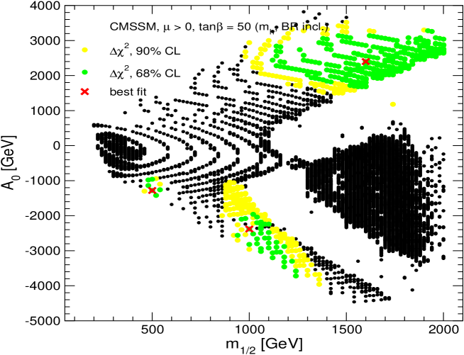
Figure 19: The results of a $\chi^{2}$ fit based on the prospective experimental accuracies for the precision observables $M_{W}$, $\sin^{2}\theta_{\mathrm{eff}}$, $(g-2)_{\mu}$, ${\rm BR}(b\to s\gamma)$, $M_{h}$ and Higgs branching ratios at the ILC are shown in the ($m_{1/2},A_{0}$) plane of the CMSSM with WMAP constraints for $\tan\beta=50$. In both plots the WMAP-allowed region and the best-fit point for $\tan\beta=50$ according to the current situation (see Fig. 15) are indicated. In both plots two further hypothetical future ‘best-fit’ values have been chosen for illustration. The coloured regions correspond to the 68% and 90% C.L. regions according to the ILC accuracies.

In each figure we show two plots, where the WMAP-allowed region and the best-fit point according to the current situation (see Fig. 15) are indicated. In both plots two further hypothetical future ‘best-fit’ points have been chosen for illustration. For all the ‘best-fit’ points, the assumed central experimental values of the observables have been chosen such that they precisely coincide with the ‘best-fit’ points. The coloured regions correspond to the 68% and 90% C.L. regions around each of the ‘best-fit’ points according to the ILC accuracies.

The comparison of Figs. 18, 19 with the result of the current fit, Fig. 15, shows that the ILC experimental precision will lead to a drastic improvement in the sensitivity to $m_{1/2}$ and $A_{0}$ when comparing precision data with the CMSSM predictions. For the best-fit values of the current fits for $\tan\beta=10$ and $\tan\beta=50$, the ILC precision would allow one to narrow down the allowed CMSSM parameter space to very small regions in the ($m_{1/2},A_{0}$) plane. The comparison of these indirect predictions for $m_{1/2}$ and $A_{0}$ with the information from the direct detection of supersymmetric particles would provide a stringent test of the CMSSM framework at the loop level. A discrepancy could indicate that supersymmetry is realised in a more complicated way than is assumed in the CMSSM.

Because of the decoupling property of supersymmetric theories, the indirect constraints become weaker for increasing $m_{1/2}$. The additional hypothetical ‘best-fit’ points shown in Figs. 18, 19 illustrate the indirect sensitivity to the CMSSM parameters in scenarios where the precision observables prefer larger values of $m_{1/2}$.

For $\tan\beta=10$, we have investigated hypothetical ‘best-fit’ values for $m_{1/2}$ of 500 GeV, 700 GeV (for $A_{0}>0$ and $A_{0}<0$) and 900 GeV. For $m_{1/2}=500\,\,\mathrm{GeV}$, the 90% C.L. region in the ($m_{1/2},A_{0}$) plane is significantly larger than for the current best-fit value of $m_{1/2}\approx 300\,\,\mathrm{GeV}$, but interesting limits can still be set on both $m_{1/2}$ and $A_{0}$. For $m_{1/2}=700\,\,\mathrm{GeV}$ and $m_{1/2}=900\,\,\mathrm{GeV}$, the 90% C.L. region extends up to the boundary of the WMAP-allowed parameter space for $m_{1/2}$. Even for these large values of $m_{1/2}$, however, the precision observables (in particular the observables in the Higgs sector) still allow one to constrain $A_{0}$.

For $\tan\beta=50$, where the WMAP-allowed region extends up to much higher values of $m_{1/2}$ , we find that for a ‘best-fit’ value of $m_{1/2}$ as large as 1 TeV, which would lie close to the LHC limit and beyond the direct-detection reach of the ILC, the precision data would still allow one to establish an upper bound on $m_{1/2}$ within the WMAP-allowed region. Thus, this indirect sensitivity to $m_{1/2}$ could give important hints for supersymmetry searches at higher-energy colliders. For ‘best-fit’ values of $m_{1/2}$ in excess of 1.5 TeV, on the other hand, the indirect effects of heavy sparticles become so small that they are difficult to resolve even with ILC accuracies.

6 Conclusions

We have investigated the sensitivity of precision observables, now and at the ILC, to indirect effects of supersymmetry within the CMSSM. We have taken into account the constraints from WMAP and other astrophysical and cosmological data which effectively reduces the dimensionality of the CMSSM parameter space.

We have performed a $\chi^{2}$ analysis based on the present experimental results of the observables $M_{W}$, $\sin^{2}\theta_{\mathrm{eff}}$, $(g-2)_{\mu}$ and ${\rm BR}(b\to s\gamma)$ for two values of $\tan\beta$, taking into account the current theoretical uncertainties. For $\tan\beta=10$, we find that the CMSSM provides a very good description of the data. A clear preference can be seen for relatively small values of $m_{1/2}$, with a best-fit value of about 300 GeV and $A_{0}\approx-m_{1/2}$. This result can be understood from the separate analyses of each of the observables, each of which is well described by the CMSSM prediction for $m_{1/2}\approx 300\,\,\mathrm{GeV}$. At the 90% C.L., we find an upper bound on $m_{1/2}$ of about 600 GeV. The supersymmetric particle spectrum corresponding to the best-fit region contains relatively light states. There is a possibility that some sparticles might be detectable at the Tevatron collider, and many should be detectable at the LHC [83] and the ILC [2], allowing a detailed determination of their properties [93].

For $\tan\beta=50$, the quality of the fit is worse than for the case with $\tan\beta=10$. While $M_{W}$ and $\sin^{2}\theta_{\mathrm{eff}}$ prefer small values of $m_{1/2}$ also for $\tan\beta=50$, $(g-2)_{\mu}$ and ${\rm BR}(b\to s\gamma)$ are better described in this case by larger $m_{1/2}$ values. The indirect constraints on $m_{1/2}$ are therefore less pronounced for $\tan\beta=50$. The best-fit value is obtained for $m_{1/2}\approx 500\,\,\mathrm{GeV}$ and negative $A_{0}$. The best-fit values for the LSP mass and the lighter stau are still below about 250 GeV, while the preferred mass values of the heavier neutralinos, the charginos and the other sleptons are in the region of 500 GeV. The 90% C.L. regions of these masses extend beyond 1 TeV, but would be kinematically accessible at a multi-TeV linear collider [94]. Coloured particles, such as the stops and sbottoms and the gluino are likely to have masses within the reach of the LHC. However, at the 90% C.L. also masses beyond $\sim 3\,\,\mathrm{TeV}$ are possible. Heavy Higgs bosons might also be accessible at the LHC in the case of large $\tan\beta$.

We have investigated the implications of our fit results for the prospects for detecting a signal for ${\rm BR}(B_{s}\to\mu^{+}\mu^{-})$. For both $\tan\beta=10$ and $\tan\beta=50$, we find that the 90% C.L. region for $m_{1/2}$ and $A_{0}$ leads to predicted values of ${\rm BR}(B_{s}\to\mu^{+}\mu^{-})$ that are below our 95% C.L. estimate of the Tevatron sensitivity at the end of Run II. With a more optimistic estimate, the Tevatron could probe a part of the parameter region for $\tan\beta=50$ at the 90% C.L. It seems more likely, however, that detection of this process would have to await LHC data.

In the second part of our analysis, we have investigated the future sensitivities of the precision observables to indirect effects of supersymmetry, assuming the experimental accuracies achievable at the ILC with a low-energy option running at the $Z$ resonance and the $WW$ threshold and estimating the future theoretical uncertainties. As further precision observables besides the ones discussed for the present situation, we have included the mass of the lightest ${\cal CP}$-even Higgs boson and the ratio of branching ratios ${\rm BR}(h\to b\bar{b})/{\rm BR}(h\to WW^{*})$. We have chosen several points in the ($m_{1/2},A_{0}$) plane of the CMSSM with the current WMAP constraints as examples for ‘best-fit’ values, adjusting the assumed future experimental central values of the precision observables to coincide with the predictions of the ‘best-fit’ values. With the prospective ILC accuracies, the sensitivity to indirect effects of supersymmetry improves very significantly compared to the present situation. We find that for assumed ‘best-fit’ values of $m_{1/2}\;\raisebox{-3.00003pt}{$\stackrel{{\scriptstyle\displaystyle<}}{{\sim}}$}\;500\,\,\mathrm{GeV}$ the precision observables allow one to constrain tightly $m_{1/2}$ and $A_{0}$. Comparing these indirect predictions with the results from the direct observation of supersymmetric particles will allow a stringent consistency test of the model at the loop level.

Because of the decoupling property of supersymmetric theories, the indirect constraints become weaker for larger $m_{1/2}$. Nevertheless, useful limits on $m_{1/2}$ and $A_{0}$ can be obtained for ‘best-fit’ values of $m_{1/2}$ as high as 1 TeV. Thus, the indirect sensitivity from the measurement of precision observables at the ILC may even exceed the direct search reach of the LHC and ILC.

Whilst this analysis has been restricted to the CMSSM, similar conclusions are expected to apply if the assumption of universal soft supersymmetry-breaking scalar masses is relaxed for the Higgs bosons, at least for values of $\mu$ and $m_{A}$ not greatly different from those in the CMSSM. The impact of the dark-matter constraint may well be rather different if universality between the soft supersymmetry-breaking squark and slepton masses is also relaxed, but we expect that the indication found here for relatively light sparticle masses would be maintained. The investigation of these issues requires a more detailed study of models beyond the CMSSM, which is in preparation.

Acknowledgements

We thank R. Clare, B. Heinemann, G. Hiller, T. Kamon and C. Weiser for useful discussions. G.W. thanks the CERN Theory Division for kind hospitality during the final stages of preparing this paper.

References

-
[1]
G. Altarelli and M. Grünewald,
hep-ph/0404165; updated in:
F. Teubert, talk given at ICHEP04, Beijing, China, August 2004, see:
ichep04.ihep.ac.cn/data/ichep04/ppt/plenary/p21-teubert-f.ppt ;
see also: lepewwg.web.cern.ch/LEPEWWG/Welcome.html . -
[2]
J. Aguilar-Saavedra et al.,
TESLA TDR Part 3:
“Physics at an Linear Collider”,
hep-ph/0106315,
see: tesla.desy.de/tdr/ ;
T. Abe et al. [American Linear Collider Working Group Collaboration], Resource book for Snowmass 2001, hep-ex/0106056;
K. Abe et al. [ACFA Linear Collider Working Group Collaboration], hep-ph/0109166. -
[3]
W. de Boer, A. Dabelstein, W. Hollik, W. Mösle
and U. Schwickerath,
Z. Phys. C 75 (1997) 627,
hep-ph/9607286;
hep-ph/9609209;
W. de Boer, M. Huber, C. Sander and D. Kazakov, Phys. Lett. B 515 (2001) 283;
W. de Boer and C. Sander, Phys. Lett. B 585 (2004) 276, hep-ph/0307049. - [4] D. Pierce and J. Erler, Nucl. Phys. Proc. Suppl. 62 (1998) 97, hep-ph/9708374; Nucl. Phys. B 526 (1998) 53, hep-ph/9801238.
-
[5]
G. Cho, K. Hagiwara, C. Kao and R. Szalapski,
hep-ph/9901351;
G. Cho and K. Hagiwara, Nucl. Phys. B 574 (2000) 623, hep-ph/9912260; Phys. Lett. B 514 (2001) 123, hep-ph/0105037. - [6] J. Erler, S. Heinemeyer, W. Hollik, G. Weiglein and P.M. Zerwas, Phys. Lett. B 486 (2000) 125; hep-ph/0005024.
- [7] W. de Boer, M. Huber, C. Sander and D. Kazakov, hep-ph/0106311.
- [8] A. Djouadi, M. Drees and J. Kneur, JHEP 0108 (2001) 055, hep-ph/0107316.
- [9] G. Belanger, F. Boudjema, A. Cottrant, A. Pukhov and A. Semenov, hep-ph/0407218.
-
[10]
C. Bennett et al.,
Astrophys. J. Suppl. 148 (2003) 1,
astro-ph/0302207;
D. Spergel et al. [WMAP Collaboration], Astrophys. J. Suppl. 148 (2003) 175, astro-ph/0302209. -
[11]
H. Goldberg,
Phys. Rev. Lett. 50 (1983) 1419;
J. Ellis, J. Hagelin, D. Nanopoulos, K. Olive and M. Srednicki, Nucl. Phys. B 238 (1984) 453. - [12] J. Ellis, K. Olive, Y. Santoso and V. Spanos, Phys. Lett. B 565 (2003) 176, hep-ph/0303043.
-
[13]
U. Chattopadhyay, A. Corsetti and P. Nath,
Phys. Rev. D 68 (2003) 035005,
hep-ph/0303201;
H. Baer and C. Balazs, JCAP 0305, 006 (2003), hep-ph/0303114;
A. Lahanas and D. Nanopoulos, Phys. Lett. B 568, 55 (2003), hep-ph/0303130;
R. Arnowitt, B. Dutta and B. Hu, hep-ph/0310103. - [14] M. Battaglia et al., Eur. Phys. J. C 22 (2001) 535, hep-ph/0106204.
- [15] B. Allanach et al., Eur. Phys. J. C 25 (2002) 113, hep-ph/0202233.
- [16] M. Battaglia, A. De Roeck, J. Ellis, F. Gianotti, K. Olive and L. Pape, Eur. Phys. J. C 33 (2004) 273, hep-ph/0306219.
- [17] H. Baer, A. Belyaev, T. Krupovnickas and X. Tata, JHEP 0402 (2004) 007, hep-ph/0311351.
- [18] J. Ellis, K. Olive, Y. Santoso and V. Spanos, hep-ph/0408118.
- [19] B. Allanach, G. Belanger, F. Boudjema and A. Pukhov, hep-ph/0410091.
- [20] J. Ellis, K. Olive, Y. Santoso and V. Spanos, Phys. Rev. D 69 (2004) 095004, hep-ph/0310356.
-
[21]
V. Abazov et al. [D0 Collaboration],
Nature 429 (2004) 638,
hep-ex/0406031;
P. Azzi et al. [CDF Collaboration, D0 Collaboration], hep-ex/0404010. -
[22]
A. Romanino and A. Strumia,
Phys. Lett. B 487 (2000) 165,
hep-ph/9912301;
J. Ellis and K. Olive, Phys. Lett. B 514 (2001) 114, hep-ph/0105004. - [23] J. Ellis, D. Nanopoulos and K. Olive, Phys. Lett. B 508 (2001) 65, hep-ph/0102331.
-
[24]
A. Sirlin,
Phys. Rev. D 22 (1980) 971;
W. Marciano and A. Sirlin, Phys. Rev. D 22 (1980) 2695. - [25] P. Chankowski, A. Dabelstein, W. Hollik, W. Mösle, S. Pokorski and J. Rosiek, Nucl. Phys. B 417 (1994) 101.
- [26] D. Garcia and J. Solà, Mod. Phys. Lett. A 9 (1994) 211.
-
[27]
A. Djouadi and C. Verzegnassi,
Phys. Lett. B 195 (1987) 265;
A. Djouadi, Nuovo Cim. A 100 (1988) 357. -
[28]
B. Kniehl,
Nucl. Phys. B 347 (1990) 89;
F. Halzen and B. Kniehl, Nucl. Phys. B 353 (1991) 567;
B. Kniehl and A. Sirlin, Nucl. Phys. B 371 (1992) 141; Phys. Rev. D 47 (1993) 883. -
[29]
K. Chetyrkin, J.H. Kühn and M. Steinhauser,
Phys. Rev. Lett. 75 (1995) 3394,
hep-ph/9504413;
L. Avdeev et al., Phys. Lett. B 336 (1994) 560, [Erratum-ibid. B 349 (1995) 597], hep-ph/9406363. - [30] K. Chetyrkin, J.H. Kühn and M. Steinhauser, Nucl. Phys. B 482 (1996) 213, hep-ph/9606230.
- [31] A. Djouadi, P. Gambino, S. Heinemeyer, W. Hollik, C. Jünger and G. Weiglein, Phys. Rev. Lett. 78 (1997) 3626, hep-ph/9612363; Phys. Rev. D 57 (1998) 4179, hep-ph/9710438.
- [32] S. Heinemeyer and G. Weiglein, JHEP 0210 (2002) 072, hep-ph/0209305; hep-ph/0301062.
-
[33]
M. Awramik, M. Czakon, A. Freitas and G. Weiglein,
Phys. Rev. D 69 (2004) 053006,
hep-ph/0311148;
G. Weiglein, Eur. Phys. J. C 33 (2004) S630, hep-ph/0312314. -
[34]
S. Heinemeyer and G. Weiglein,
hep-ph/0307177;
S. Heinemeyer, Nucl. Phys. Proc. Suppl. 135, 114 (2004) hep-ph/0406245. -
[35]
F. Jegerlehner,
Talk presented at the LNF Spring School,
Frascati, Italy, 1999, see:
www.ifh.de/fjeger/Frascati99.ps.gz ; hep-ph/0105283. - [36] S. Heinemeyer, S. Kraml, W. Porod and G. Weiglein, JHEP 0309 (2003) 075, hep-ph/0306181.
- [37] G. Wilson, LC-PHSM-2001-009, see: www.desy.de/lcnotes/notes.html .
- [38] U. Baur, R. Clare, J. Erler, S. Heinemeyer, D. Wackeroth, G. Weiglein and D. Wood, hep-ph/0111314.
- [39] M. Awramik, M. Czakon, A. Freitas and G. Weiglein, to appear in Phys. Rev. Lett., hep-ph/0407317.
- [40] R. Hawkings and K. Mönig, Eur. Phys. J. direct C 8 (1999) 1, hep-ex/9910022.
- [41] A. Czarnecki and W. Marciano, Phys. Rev. D 64 (2001) 013014, hep-ph/0102122.
- [42] M. Knecht, hep-ph/0307239.
- [43] M. Davier, S. Eidelman, A. Höcker and Z. Zhang, Eur. Phys. J. C 31 (2003) 503, hep-ph/0308213.
- [44] K. Hagiwara, A. Martin, D. Nomura and T. Teubner, Phys. Rev. D 69 (2004) 093003, hep-ph/0312250.
- [45] S. Ghozzi and F. Jegerlehner, Phys. Lett. B 583 (2004) 222, hep-ph/0310181.
- [46] J. de Troconiz and F. Yndurain, hep-ph/0402285.
-
[47]
M. Knecht and A. Nyffeler,
Phys. Rev. D 65 (2002) 073034,
hep-ph/0111058;
M. Knecht, A. Nyffeler, M. Perrottet and E. De Rafael, Phys. Rev. Lett. 88 (2002) 071802, hep-ph/0111059;
I. Blokland, A. Czarnecki and K. Melnikov, Phys. Rev. Lett. 88 (2002) 071803, hep-ph/0112117;
M. Ramsey-Musolf and M. Wise, Phys. Rev. Lett. 89 (2002) 041601, hep-ph/0201297;
J. Kühn, A. Onishchenko, A. Pivovarov and O. Veretin, Phys. Rev. D 68 (2003) 033018, hep-ph/0301151. - [48] K. Melnikov and A. Vainshtein, hep-ph/0312226.
- [49] A. Aloisio et al. [KLOE Collaboration], hep-ex/0407048.
- [50] A. Hocker, hep-ph/0410081.
- [51] T. Kinoshita and M. Nio, hep-ph/0402206.
- [52] [The Muon g-2 Collaboration], Phys. Rev. Lett. 92 (2004) 161802, hep-ex/0401008.
- [53] T. Moroi, Phys. Rev. D 53 (1996) 6565 [Erratum-ibid. D 56 (1997) 4424], hep-ph/9512396.
- [54] G. Degrassi and G. Giudice, Phys. Rev. D 58 (1998) 053007, hep-ph/9803384.
- [55] S. Heinemeyer, D. Stöckinger and G. Weiglein, Nucl. Phys. B 690 (2004) 62, hep-ph/0312264.
- [56] S. Heinemeyer, W. Hollik and G. Weiglein, Comp. Phys. Comm. 124 2000 76, hep-ph/9812320; Eur. Phys. J. C 9 (1999) 343, hep-ph/9812472. The codes are accessible via www.feynhiggs.de .
-
[57]
S. Heinemeyer,
hep-ph/0407244;
T. Hahn, S. Heinemeyer, W. Hollik and G. Weiglein, MPP–2003–147, in proceedings of Physics at TeV Colliders, Les Houches, June 2003, hep-ph/0406152; in preparation. - [58] S. Heinemeyer, D. Stöckinger and G. Weiglein, Nucl. Phys. B 699 (2004) 103, hep-ph/0405255.
- [59] S. Heinemeyer, W. Hollik and G. Weiglein, hep-ph/0412214.
-
[60]
K. Adel and Y. Yao,
Phys. Rev. D 49 (1994) 4945,
hep-ph/9308349;
C. Greub, T. Hurth and D. Wyler, Phys. Lett. B 380 (1996) 385, hep-ph/9602281; Phys. Rev. D 54 (1996) 3350, hep-ph/9603404;
K. Chetyrkin, M. Misiak and M. Münz, Phys. Lett. B 400, (1997) 206, [Erratum-ibid. B 425 (1998) 414] hep-ph/9612313;
P. Gambino and M. Misiak, Nucl. Phys. B 611 (2001) 338, hep-ph/0104034;
A. Ali, talk given at ICHEP04, Beijing, August 2004, to appear in the proceedings, see: ichep04.ihep.ac.cn/db/paper.php . -
[61]
R. Barate et al. [ALEPH Collaboration],
Phys. Lett. B 429 (1998) 169;
S. Chen et al. [CLEO Collaboration], Phys. Rev. Lett. 87 (2001) 251807, hep-ex/0108032;
P. Koppenburg et al. [Belle Collaboration], Phys. Rev. Lett. 93 (2004) 061803, hep-ex/0403004;
K. Abe et al. [Belle Collaboration], Phys. Lett. B 511 (2001) 151, hep-ex/0103042;
B. Aubert et al. [BABAR Collaboration], hep-ex/0207074; hep-ex/0207076;
see also www.slac.stanford.edu/xorg/hfag/ . - [62] C. Degrassi, P. Gambino and G. Giudice, JHEP 0012 (2000) 009, hep-ph/0009337.
- [63] P. Gambino and M. Misiak, Nucl. Phys. B 611 (2001) 338, hep-ph/0104034.
-
[64]
P. Cho, M. Misiak and D. Wyler,
Phys. Rev. D 54, 3329 (1996),
hep-ph/9601360;
A. Kagan and M. Neubert, Eur. Phys. J. C 7 (1999) 5, hep-ph/9805303;
K. Chetyrkin, M. Misiak and M. Münz, Phys. Lett. B 400, (1997) 206, [Erratum-ibid. B 425 (1998) 414] hep-ph/9612313;
A. Ali, E. Lunghi, C. Greub and G. Hiller, Phys. Rev. D 66 (2002) 034002, hep-ph/0112300;
G. Hiller and F. Krüger, Phys. Rev. D 69 (2004) 074020, hep-ph/0310219. - [65] G. Belanger, F. Boudjema, A. Pukhov and A. Semenov, Comput. Phys. Comm. 149 (2002) 103, hep-ph/0112278; hep-ph/0405253.
-
[66]
G. Buchalla and A. Buras,
Nucl. Phys. B 400 (1993) 225;
M. Misiak and J. Urban, Phys. Lett. B 451 (1999) 161, hep-ph/9901278;
G. Buchalla and A. Buras, Nucl. Phys. B 548 (1999) 309, hep-ph/9901288;
A. Buras, Phys. Lett. B 566 (2003) 115, hep-ph/0303060. - [67] M. Herndon, talk given at ICHEP04, Beijing, August 2004, to appear in the proceedings, see: ichep04.ihep.ac.cn/db/paper.php .
- [68] B. Heinemann, talk given at IDM04, Edinburgh, September 2004, to appear in the proceedings, see: www.shef.ac.uk/physics/idm2004.html .
- [69] P. Ball et al., hep-ph/0003238.
-
[70]
K. Babu and C. Kolda,
Phys. Rev. Lett. 84 (2000) 228,
hep-ph/9909476;
S. Choudhury and N. Gaur, Phys. Lett. B 451 (1999) 86, hep-ph/9810307;
C. Bobeth, T. Ewerth, F. Krüger and J. Urban, Phys. Rev. D 64 (2001) 074014, hep-ph/0104284;
A. Dedes, H. Dreiner and U. Nierste, Phys. Rev. Lett. 87 (2001) 251804, hep-ph/0108037;
G. Isidori and A. Retico, JHEP 0111 (2001) 001, hep-ph/0110121;
A. Dedes and A. Pilaftsis, Phys. Rev. D 67 (2003) 015012, hep-ph/0209306;
A. Buras, P. Chankowski, J. Rosiek and L. Slawianowska, Nucl. Phys. B 659 (2003) 3, hep-ph/0210145;
A. Dedes, Mod. Phys. Lett. A 18 (2003) 2627, hep-ph/0309233. -
[71]
Y. Okada, M. Yamaguchi, T. Yanagida,
Prog. Theor. Phys. 85 (1991) 1;
J. Ellis, G. Ridolfi, F. Zwirner, Phys. Lett. B 257 (1991) 83;
H. Haber, R. Hempfling, Phys. Rev. Lett. 66 (1991) 1815. - [72] P. Chankowski, S. Pokorski, J. Rosiek, Phys. Lett. B 286 (1992) 307; Nucl. Phys. B 423 (1994) 437, hep-ph/9303309.
- [73] A. Dabelstein, Nucl. Phys. B 456 (1995) 25, hep-ph/9503443; Z. Phys. C 67 (1995) 495, hep-ph/9409375.
- [74] G. Degrassi, S. Heinemeyer, W. Hollik, P. Slavich, G. Weiglein, Eur. Phys. J. C 28 (2003) 133, hep-ph/0212020.
-
[75]
M. Carena, D. Garcia, U. Nierste and C. Wagner,
Nucl. Phys. B 577 (2000) 577,
hep-ph/9912516;
H. Eberl, K. Hidaka, S. Kraml, W. Majerotto and Y. Yamada, Phys. Rev. D 62 (2000) 055006, hep-ph/9912463. -
[76]
T. Banks,
Nucl. Phys. B 303 (1988) 172;
L. Hall, R. Rattazzi and U. Sarid, Phys. Rev. D 50 (1994) 7048, hep-ph/9306309;
R. Hempfling, Phys. Rev. D 49 (1994) 6168;
M. Carena, M. Olechowski, S. Pokorski and C. Wagner, Nucl. Phys. B 426 (1994) 269, hep-ph/9402253. - [77] G. Degrassi, A. Dedes, P. Slavich, Nucl. Phys. B 672 (2003) 144, hep-ph/0305127.
-
[78]
S. Martin,
Phys. Rev. D 66 (2002) 096001,
hep-ph/0206136;
D 67 (2003) 095012, hep-ph/0211366; D 68 075002 (2003), hep-ph/0307101; D 70 (2004) 016005, hep-ph/0312092; hep-ph/0405022. - [79] S. Heinemeyer, W. Hollik, H. Rzehak and G. Weiglein, to appear in Eur. Phys. J. C, hep-ph/0411114.
- [80] S. Heinemeyer, W. Hollik and G. Weiglein, JHEP 0006 (2000) 009, hep-ph/9909540.
-
[81]
J. Ellis, S. Heinemeyer, K. Olive and G. Weiglein,
Phys. Lett. B 515 (2001) 348,
hep-ph/0105061;
JHEP 0301 (2003) 006,
hep-ph/0211206;
S. Ambrosanio, A. Dedes, S. Heinemeyer, S. Su and G. Weiglein, Nucl. Phys. B 624 (2001) 3, hep-ph/0106255;
A. Dedes, S. Heinemeyer, S. Su and G. Weiglein, Nucl. Phys. B 674 (2003) 271, hep-ph/0302174. -
[82]
D. Zeppenfeld, R. Kinnunen, A. Nikitenko and
E. Richter-Was,
Phys. Rev. D 62 (2000) 013009,
hep-ph/0002036;
A. Belyaev and L. Reina, JHEP 0208 (2002) 041, hep-ph/0205270;
M. Dührssen, S. Heinemeyer, H. Logan, D. Rainwater, G. Weiglein and D. Zeppenfeld, Phys. Rev. D 70 (2004) 113009, hep-ph/0406323. -
[83]
ATLAS Collaboration,
Detector and Physics Performance Technical Design Report,
CERN/LHCC/99-15 (1999), see:
atlasinfo.cern.ch/Atlas/GROUPS/PHYSICS/TDR/access.html ;
CMS Collaboration, see:
cmsinfo.cern.ch/Welcome.html/CMSdocuments/CMSplots/ . - [84] M. Dührssen, ATL-PHYS-2003-030, available from cdsweb.cern.ch .
- [85] K. Desch, E. Gross, S. Heinemeyer, G. Weiglein and L. Zivkovic, JHEP 0409 (2004) 062, hep-ph/0406322.
- [86] S. Heinemeyer, W. Hollik and G. Weiglein, Eur. Phys. J. C 16 (2000) 139, hep-ph/0003022.
- [87] T. Barklow, hep-ph/0312268.
- [88] LEP Higgs working group, Phys. Lett. B 565 (2003) 61, hep-ex/0306033.
- [89] LEP Higgs working group, hep-ex/0107030; hep-ex/0107031; LHWG-Note 2004-01, see: lephiggs.web.cern.ch/LEPHIGGS/papers/ .
- [90] S. Eidelman et al. [Particle Data Group Collaboration], Phys. Lett. B 592 (2004) 1.
- [91] B. Heinemann and T. Kamon, private communications.
-
[92]
D. Denegri et al.,
hep-ph/0112045;
D. Cavalli et al., hep-ph/0203056. - [93] G. Weiglein et al. [LHC / LC Study Group], hep-ph/0410364.
- [94] CLIC Physics Workging Group, hep-ph/0412251.