QCD Phenomenology of Static Sources

Abstract

We discuss the spectrum of open string and point particle excitations in QCD with various source representations. Some general relations are introduced and lattice results presented. In particular we discuss the short-distance behaviour, relate this to perturbation theory expectations and comment on the matching between low energy matrix elements and high energy Wilson coefficients, within the framework of effective field theories.

1 Introduction

We discuss the excitation spectrum of QCD in its static limit. This is quite amusing, in the context of a Light Cone Workshop. However, some of the results are instructive and of a very general nature, in particular those concerning the spectrum of QCD and the question of power divergences and renormalons. For instance the Wilson-Schwinger line appears at prominent places. We shall see that in a scheme without a hard cut-off, such as dimensional regularisation (DR), such objects require special attention. Wilson lines do not only appear in the static limit, within the framework of heavy quark effective field theories, but for instance also within light cone parton distributions [1], if one wishes to define them in a gauge invariant (and hopefully path-independent) way [2, 3, 4].

In general, a Wilson-Schwinger line of length $l$ in Euclidean space-time within a correlation function will result in a term $\propto\exp(-\overline{\Lambda}l)$, with some self-energy $\overline{\Lambda}$. In DR any perturbative contribution to $\overline{\Lambda}$ vanishes. This is different in schemes with a hard momentum cut-off, such as lattice regularisation. In this case $\overline{\Lambda}$ contains a contribution that is proportional to the inverse lattice spacing $a^{-1}$ and which can be expanded in powers of $\alpha_{s}$. Within physical observables such power terms obviously have to cancel.

To translate $\overline{\Lambda}$ from the lattice into the on-shell (OS) scheme the perturbative expansion of $\overline{\Lambda}$ has to be subtracted, replacing the $a^{-1}$ term by a renormalon ambiguity. For physical observables to remain unaffected, the renormalon of $\overline{\Lambda}$ in the OS scheme has to cancel against a similar renormalon associated with a different term. One nice thing about a hard cut-off is that the structure of power terms within such a regularisation scheme is indicative of the renormalon structure that one will encounter in a DR calculation. One way of elucidating this connection has been explained above: the price of cancelling a power term is a renormalon. Vice versa it is possible to remove (part of) such a renormalon, by introducing a scale dependence and replacing it by a power term. One such continuum scheme, the RS scheme, has been suggested in refs. [5, 6].

Here I discuss the spectrum of QCD in the static limit. The simplest case would be that of a static-light meson. In the continuum limit the mass $\overline{\Lambda}$ of such a particle will diverge. Only level splittings are well defined. One can however, relate this mass to the mass of the physical $B$ meson, within Heavy Quark Effective Theory (HQET). In this case the power term/renormalon of $\overline{\Lambda}$ will be compensated for by a similar contribution to $m_{b}$.

This article is organised as follows: in Section 2 we introduce the relevant correlation functions and discuss some fundamental relations. Then in Section 3 we survey some aspects of the large distance behaviour and string breaking, before we discuss short distance relations in Section 4.

2 Static QCD strings and particles: the broad picture

We discuss the spectrum of QCD with one or two static charges, where we restrict ourselves to charges in the fundamental representation, ${\mathbf{3}}$, and the adjoint representation, ${\mathbf{8}}$. The former can be motivated as representing the starting point for realising a heavy quark within an effective field theory such as HQET, non-relativistic QCD (NRQCD) or potential NRQCD (pNRQCD) [7, 8]. The adjoint representation can be used to describe a gluino, within a heavy-gluino expansion (should a gluino exist and be sufficiently stable).

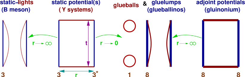
Figure 1: Correlation functions in the static sector of QCD.

We schematically depict the correlation functions $C(r,t)$ that we investigate in Fig. 1. The states are created at time $0$ and destroyed at time $t$. Straight spatial lines are parallel transporters, straight temporal lines static propagators (Wilson-Schwinger lines) in fundamental or adjoint representation. Curved lines represent sea quarks and gluons. The corresponding (in most cases $r$-dependent) energy levels can be extracted in the limit of large Euclidean times,

$$E(r)=-\lim_{t\rightarrow\infty}\frac{d\ln C(r,t)}{dt}.$$ (1)

We denote the energy level of a static-light meson by,

$$M_{B}=m_{b}+\overline{\Lambda}+O(1/m_{b}),$$ (2)

where both the quark mass $m_{b}$ and the binding energy (or static energy) $\overline{\Lambda}$ are scheme- and scale-dependent, in reflection of the fact that asymptotic states cannot carry strong charge. $M_{B}$ however is a physical observable. Note that $m_{b}$ does not appear as a scale in the static limit. I introduce it nonetheless for pedagogical reasons. Taking account of light quark spin and angular momentum the spectrum of $\overline{\Lambda}$ is arranged in spin-doublets $(n+\frac{1}{2})^{\pm}$ where for instance $\frac{1}{2}^{-}$ corresponds to $l=0$ and $\frac{1}{2}^{+}$ to $l=1$. The presence of such spin doublets has found an exciting application, with the recent discovery of two new $D_{s}$ states [9, 10, 11, 12]. Once $1/m_{b}$ corrections are added, the heavy quark spin has to be taken into account and the $\frac{1}{2}^{-}$ ground state will further split into a pseudoscalar $B$ meson and a vector $B^{*}$ meson.

The next step is an open string state, between a fundamental source and anti-source separated by a distance $r$. In this case the inclusion of $1/m_{b}$ corrections is essential, even at leading order as without a kinetic term all sorts of pathologies can arise which are related to the fact that heavy quarks at relative speed decouple from each other. The more conceptional results presented here are not affected by this problem. One encounters a ground state $E_{s}(r)$ as well as hybrid excitations $E_{H}(r)$, due to radial and/or orbital gluonic excitations. Obviously, sea quarks screen these potentials and,

$$\lim_{r\rightarrow\infty}E_{s}(r)=2M_{B},$$ (3)

which is known as “string breaking”. Note that the heavy quark mass $m_{b}$ cancels from the combination, $E_{s}(r)-2M_{B}$. A similar relation will apply to $E_{H}$, which will also decay, depending on the quantum numbers $H$, into a pair of $B$ mesons.

Within the framework of pNRQCD which amounts to a double expansion both in the relative quark velocity (NRQCD) and in the distance $r$, one can classify the short distance behaviour. In the static limit the only scale, apart from a typical non-perturbative QCD scale $\Lambda_{QCD}$, is the distance $r$ and one can identify [6],

$$E_{s}(r) = 2m_{b}+V_{s}(r)+O(r^{2})=2m_{b}^{L}+E_{s}^{L}(r),$$ (4)

$$E_{H}(r) = 2m_{b}+V_{o}(r)+\Lambda_{H}+O(r^{2})=2m_{b}^{L}+E_{H}^{L}(r),$$ (5)

where both, singlet and octet potentials $V_{s}(r)$ and $V_{o}(r)$ are calculable in perturbation theory for distances, $r\ll\Lambda_{QCD}^{-1}$. $\Lambda_{H}$ stands for the mass of a gluelump (see below). Again, $m_{b}$, $V_{s}(r)$, $V_{o}(r)$ and $\Lambda_{H}$ are scheme and scale dependent. The new ingredient now is that the definition of the infrared gluelump energy $\Lambda_{H}$ carries an ultraviolet renormalon ambiguity that has to be compensated for by $V_{o}$. The ultraviolet ambiguity of $V_{o}$ in turn is the same as that of $V_{s}$ and related to the definition of the quark mass $m_{b}$. On the other hand one can also calculate these energy levels non-perturbatively in lattice simulations and identify these as the ground state static potential, $E_{s}^{L}(r)$ (which is in the $s=\Sigma_{g}^{+}$ representation of the cylindrical group $D_{\infty h}$) and hybrid excitations, $E_{H}^{L}(r)$.

The second equalities within Eqs. (4) and (5) above are only correct up to lattice artefacts which for the lattice actions used here will be proportional to $a^{2}\Lambda_{QCD}^{2}$ and $a^{2}/r^{2}$. The $a^{2}/r^{2}$ correction means that these relations do not hold in the limit $r\rightarrow 0$. In particular, unlike the continuum $E_{s}$, $E_{s}^{L}(0)=0$ does not diverge and $E_{H}^{L}(0)=\Lambda_{H}^{L}$. Note that in lattice schemes both $m_{b}$ and $V_{s}$ contain power divergences $\propto a^{-1}$ which cancel each other. As $r<a$ the above continuum limit interpretation is not valid anymore and $E_{s}(0)=V_{s,L}(0)=0$. The lattice “$1/r$” term within $V_{s,L}$ assumes a finite value, $\propto a^{-1}$, at $r=0$, that exactly cancels the power term of the static energy.

If we subtract the above equations from each other we obtain a consistent picture,

$$E_{H}(r)-E_{s}(r)=V_{s}(r)-V_{o}(r)+\Lambda_{H}+O(r^{2})=E_{H}^{L}(r)-E_{s}^{L}(r).$$ (6)

The second equality only applies modulo lattice artefacts, i.e. for $r\gg a$. This combination does not contain the leading renormalon and is also power term free.

As indicated in Fig. 1, in the limit $r\rightarrow 0$ the non-perturbative energy levels calculated on the lattice will either correspond to gluelumps or to glueballs, at least if we neglect sea quarks for the moment. In fact, as gluelumps are accompanied by power divergencies, at sufficiently small lattice spacing, gluelumps will always form the ground state within each $J^{PC}$ sector. Starting from these glueballs and pulling the static sources apart (${\mathbf{1}}\oplus{\mathbf{8}}={\mathbf{3}}\otimes{\mathbf{3}}^{*}$) these states can be identified as the ground state in the fundamental open string sector plus glueball scattering states. If we start from a gluelump, increasing the distance will lead us to hybrid energies (or hybrid energies plus glueballs). At $r>0$ the symmetry is reduced from $O(3)\otimes{\mathcal{C}}$ to $D_{\infty h}$ and each gluelump state will in fact be approached by more than one hybrid energy level. Note that gluelump masses are scale and scheme dependent while gluelump mass splittings are universal.

We have restricted the discussion of gluelumps and hybrid potentials to the case without sea quarks. Note however that the presence of (massive) sea quarks will not change the situation conceptionally. We have already discussed the breaking of the ground state string above and the same will happen in the hybrid sector. Sea quarks will result in $B\overline{B}$ potentials, in addition to the conventional hybrid potentials. Their presence will provide us with an alternative possibility of screening of a static octet charge by quark and antiquark and this will give rise to additional scattering states. The level orderings will somewhat change and the excitation spectrum will become more dense. However, the pNRQCD multipole expansion also provides the framework for classifying this situation and moreover the renormalon and power term structure will remain unaffected.

Finally, the gluelump energy $\Lambda_{H}$ is an object very similar to the binding energy $\overline{\Lambda}$ of a $B$ meson. Imagine a heavy gluino with mass $m_{\tilde{g}}$. This will be screened by the gluons within the QCD vacuum and only visible as a bound state glueballino with mass,

$$M_{\tilde{G}}=m_{\tilde{g}}+\Lambda_{B}+O(1/m_{\tilde{g}}).$$ (7)

The lightest glueballino will be the magnetic one, $H=1^{+-}=B$. The scheme and scale dependence of $\Lambda_{B}$ is required to cancel that of $m_{\tilde{g}}$. In a similar way in which heavy-light mesons are related to quarkonia at $r\rightarrow\infty$, glueballinos are related to gluinonia, bound states of two heavy gluinos:

$$E_{A}(r)=2m_{\tilde{g}}+V_{A,s}(r)+O(r^{2})\stackrel{{\scriptstyle r\rightarrow\infty}}{{\longrightarrow}}2M_{\tilde{G}},$$ (8)

where $V_{A,s}(r)$ is the singlet potential between two adjoint sources. As ${\mathbf{8}}\otimes{\mathbf{8}}={\mathbf{1}}\oplus{\mathbf{8}}\oplus{\mathbf{8}}\oplus{\mathbf{1}}{\mathbf{0}}\oplus{\mathbf{1}}{\mathbf{0}}^{*}\oplus{\mathbf{2}}{\mathbf{7}}$, at $r\rightarrow 0$ contact can be made between static hybrid gluinonium energy levels and gluelumps, this time not only in representation ${\mathbf{8}}$ but also in ${\mathbf{1}0}$ and ${\mathbf{2}7}$: a whole tower of states exists, and each new representation introduces a new renormalon/power term.

Unfortunately, no numerical results on hybrid excitations of non-fundamental QCD strings or of higher representation gluelumps exist thus far. However, singlet open string excitations in representations even larger than the adjoint one have for instance been calculated in ref. [13] and the closed string spectrum in ref. [14].

3 String Breaking and $m_{b}$

Attempts to resolve string breaking in lattice studies of QCD with sea quarks have a long history. While everyone knows that this effect exists, it is still a crucial benchmark for the capability of lattice calculations. Moreover, the dynamics of the mixing between open string and broken string states, which are the starting points for a description of quarkonia and heavy-light mesons, respectively, is non-trivial. This will elucidate strong quarkonium decay rates and other properties near threshold.

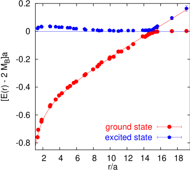
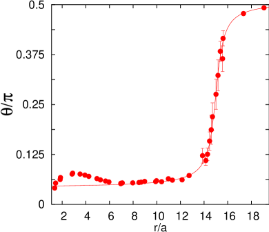
Figure 2: The lowest two energy levels in the $Q{\overline{Q}}$ system with sea quarks. On the right hand side the $\overline{B}B$ content of the ground state is shown, in terms of a mixing angle. The results apply to $n_{f}=2$, $m_{q}\approx m_{s}$ and $a\approx 0.085$ fm.

First studies in toy models were performed as soon as in 1988 [15]. Only some five years ago quantitatively satisfying results were obtained, first in $SU(2)$-Higgs models [16, 17] and then for the adjoint representation string in $SU(2)$ gauge theory [18, 19]. The latter case corresponds to the decay of gluinonium into two gluinoballs, discussed above. Several attempts on the string breaking problem in QCD with sea quarks were made [20, 21, 22, 23] but only very recently reliable results were obtained [24]. These are displayed in Fig. 2. String breaking takes place at around $r_{c}\approx 1.27$ fm for light quark masses similar to that of the strange quark. An extrapolation to physical quark masses yields $r_{c}\approx 1.16$ fm. The gap between the two states in the string breaking region is about $\Delta E\approx 50$ MeV and we are able to resolve this with a resolution of 10 standard deviations! One might expect lighter sea quarks to extend the pion exchange related “bump” in the excited energy level and mixing angle towards larger distances and also to further broaden the gap $\Delta E$.

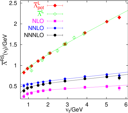
Figure 3: The binding energy $\overline{\Lambda}$ from the $Q\overline{Q}$ potential (solid diamonds) and from static-light mesons (open diamonds) as well as the perturbative conversion into the RS scheme at different orders.

We have discussed that $E_{s}(r)\rightarrow 2M_{B}$ for $r\rightarrow\infty$. This is not the case in the quenched approximation, however, still at some distance $r_{c}=1.13(7)$ fm [6, 21] we will find $\frac{1}{2}E_{s}(r_{c})=M_{B}$. On the lattice we have,

$$\frac{1}{2}E_{s}^{L}(r_{c})=\frac{1}{2}E_{s}(r_{c})-m_{b,L}=\overline{\Lambda}^{L}_{\mbox{\scriptsize pot}}.$$ (9)

One can determine both, the binding energy from the static potential, $\overline{\Lambda}^{L}_{\mbox{\scriptsize pot}}(a)=\frac{1}{2}E_{s}^{L}(0.5\,\mbox{fm};a)+\Delta$, up to a constant $\Delta$ and $\overline{\Lambda}^{L}(a)$ directly from the static-light system [25, 26, 27, 12]. The latter values are less accurate since a chiral extrapolation in the light quark mass is required. There are also inconsistencies between different $\overline{\Lambda}^{L}$ data sets obtained by different groups at the coarser lattice spacings.

The leading overall renormalon ambiguity cancels from the running of $\Lambda^{L}$ from one scale $\nu_{f}=a^{-1}$ to another. In Fig. 3 we plot the results (diamonds), together with the NNNLO perturbative expectation, expanded in terms of $\alpha_{s}(3.9\,\mbox{GeV})$. We find excellent agreement between perturbation theory and the lattice data, down to energies as low as $\nu_{f}<1$ GeV. We also translate the results into the RS scheme [5]. At large scales (small lattice spacings) the power term becomes large and hence a conversion between schemes requires very accurate perturbative coefficients. At small scales this requirement is less demanding but perturbation theory obviously becomes less convergent. AT NNNLO the optimal accuracy can be obtained around $\nu_{f}\approx 4$ GeV.

By subtracting the power term from $\overline{\Lambda}^{L}$ one obtains the binding energy in the OS scheme. This is scale independent but contains a renormalon ambiguity. If we are interested in extracting the $b$ quark mass in the $\overline{MS}$ scheme the renormalon above will cancel against the one that arises from converting the OS $b$ quark mass $m_{b,OS}(a)=M_{B}-\overline{\Lambda}^{OS}\!(a)$ into the $\overline{MS}$ mass [28]. We use the RS scheme as an intermediate scheme in this conversion and obtain [6],

$$m_{b,\overline{MS}}(m_{b,\overline{MS}})=[4191\pm 29(\mbox{stat.})\pm 47(\mbox{th.})\pm 1(\Lambda_{\overline{MS}})]\,\mbox{MeV}.$$ (10)

The theoretical error includes $1/m_{b}$ corrections. In addition to the errors displayed we expect an $O(100\,\mbox{MeV})$ quenching uncertainty.

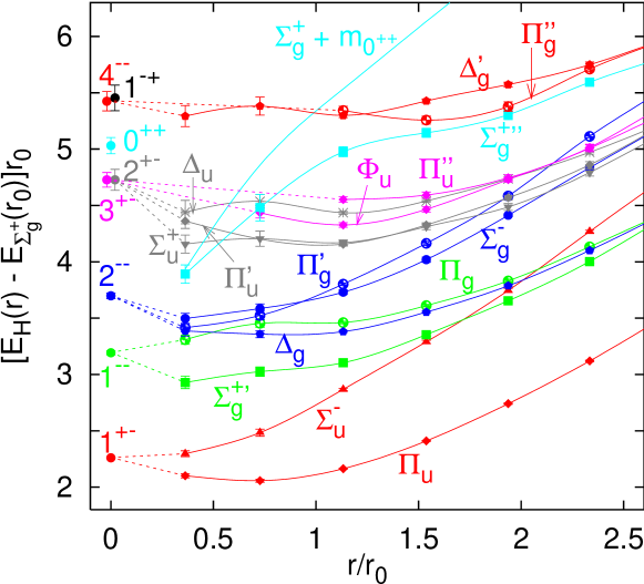
Figure 4: Hybrid energies [29], in comparison with the gluelump spectrum, extrapolated to the continuum limit [30] (circles, left-most data points). The gluelump spectrum has been shifted by an arbitrary constant to adjust the $1^{+-}$ state with the $\Pi_{u}$ and $\Sigma_{u}^{-}$ potentials at short distance. The lines are drawn to guide the eye.

4 Gluelumps and Hybrids

At short distances one would expect more than one $\Lambda_{\eta}^{\sigma_{v}}$ hybrid to approach the same $J^{PC}$ gluelump energy level where $J\geq\Lambda$ and $\eta=PC$ since $D_{\infty h}\subset O(3)\otimes{\mathcal{C}}$. Qualitatively this can be verified in Fig. 4 where we compare hybrid energies obtained in ref. [29] with the gluelump spectrum of ref. [30]. The dashed lines correspond to our expectations. Only the $\Sigma_{g}^{+\prime\prime}$ level cannot be disentangled from a glueball scattering state. Everything is displayed in units of $r_{0}\approx 0.5$ fm.

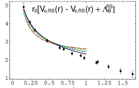
Figure 5: Splitting between the $\Pi_{u}$ and the $\Sigma_{g}^{+}$ energies. $(V_{o,\mbox{\tiny RS}}-V_{s,\mbox{\tiny RS}})(r)+\Lambda_{B}^{\mbox{\tiny RS}}$ is plotted at tree level (dashed line), one-loop (dashed-dotted line), two loops (dotted line) and three loops (estimate) plus the leading single ultrasoft log (solid line).

We calculate the lowest two hybrid potentials $E^{L}_{H}(r)$ with $H=\Pi_{u}$ and $H=\Sigma_{u}^{-}$ which both will approach the lightest (magnetic) $1^{-+}$ gluelump. According to Eq. (5), the hybrid energies are the non-perturbative generalisation of the octet potential of the perturbative multipole expansion. pNRQCD predicts the leading order difference between these two levels to be $\propto r^{2}$, which we are able to verify.

There are now two strategies of determining a gluelump mass $\Lambda_{B}$. Either one can directly calculate it at a given lattice spacing $a$ on the lattice and subsequently convert it into another scheme or one can compute the power term free combination $E_{\Pi_{u}}^{L}(r)-E^{L}_{s}(r)$ at $r\gg a$ and extrapolate the result to the continuum limit. Subsequently, one can then follow Eq. (6), subtract $V_{s}(r)-V_{o}(r)$ and obtain $\Lambda_{H}$. The result of a continuum limit extrapolation of the difference is displayed in Fig. 5, together with the expectation Eq. (6) to different orders in perturbation theory, using the RS scheme [5, 6]. The $n_{f}=0$ QCD coupling has been taken from ref. [31] and hence the only free parameter in the fit is the gluelump energy,

$$\Lambda_{B}^{\mbox{\scriptsize RS}}(1\,\mbox{GeV})=[887\pm 39(\mbox{latt.})\pm 83(\mbox{th.})\pm 32(\Lambda_{\overline{MS}})]\,\mbox{MeV}.$$ (11)

We obtain a compatible result, following the first strategy outlined above, perturbatively converting the lattice gluelump data of ref. [30] at finite lattice spacings, $\Lambda_{B}^{L}(a)$, into the RS scheme, in analogy to our determination of the static-light binding energy. The second lightest gluelump is the electric one ($1^{--}$) which is about 350–400 MeV heavier than the magnetic gluelump.

5 Conclusions

Relations between static energy levels at short and large distances (string breaking) have been reviewed. For the static energies NNLO/NNNLO $\overline{MS}$ perturbation theory works very well down to energies of less than 1 GeV, once the leading renormalon has been accounted for. Static Wilson-Schwinger lines in the fundamental and adjoint representations give rise to masses (the binding energies $\overline{\Lambda}$ and gluelumps, respectively) that are scale and scheme dependent. This has implications with respect to QCD vacuum models and condensates. In particular, when combining perturbative Wilson coefficients with non-perturbative matrix elements these have to be defined in the same scheme and at the same scale to enable renormalon cancellation.

I thank my collaborators Thomas Düssel, Thomas Lippert, Hartmut Neff, Antonio Pineda and Klaus Schilling. This work is supported by the EC Hadron Physics I3 Contract No. RII3-CT-2004-506078, by a PPARC Advanced Fellowship (grant PPA/A/S/2000/00271) as well as by PPARC grant PPA/G/0/2002/0463.

References

- [1] J. C. Collins and D. E. Soper, Nucl. Phys. B 194, 445 (1982); D. E. Soper, Phys. Rev. Lett. 43, 1847 (1979).
- [2] X.-D. Ji and F. Yuan, Phys. Lett. B 543, 66 (2002) [arXiv:hep-ph/0206057].
- [3] J. C. Collins, Acta Phys. Polon. B 34, 3103 (2003) [arXiv:hep-ph/0304122].
- [4] M. Burkardt, Nucl. Phys. A 735, 185 (2004) [arXiv:hep-ph/0302144].
- [5] A. Pineda, J. Phys. G 29, 371 (2003) [arXiv:hep-ph/0208031].
- [6] G. S. Bali and A. Pineda, Phys. Rev. D 69, 094001 (2004) [arXiv:hep-ph/0310130].
- [7] A. Pineda and J. Soto, Nucl. Phys. Proc. Suppl. 64, 428 (1998) [arXiv:hep-ph/9707481].
- [8] N. Brambilla, A. Pineda, J. Soto and A. Vairo, Nucl. Phys. B 566, 275 (2000) [arXiv:hep-ph/9907240].
- [9] M. A. Nowak, M. Rho and I. Zahed, Phys. Rev. D 48, 4370 (1993) [arXiv:hep-ph/9209272].
- [10] W. A. Bardeen and C. T. Hill, Phys. Rev. D 49, 409 (1994) [arXiv:hep-ph/9304265]; W. A. Bardeen, E. J. Eichten and C. T. Hill, Phys. Rev. D 68, 054024 (2003) [arXiv:hep-ph/0305049].
- [11] G. S. Bali, Phys. Rev. D 68, 071501 (2003) [arXiv:hep-ph/0305209].
- [12] A. M. Green et al. [UKQCD Collaboration], Phys. Rev. D 69, 094505 (2004) [arXiv:hep-lat/0312007].
- [13] G. S. Bali, Phys. Rev. D 62, 114503 (2000) [arXiv:hep-lat/0006022].
- [14] B. Lucini, M. Teper and U. Wenger, JHEP 0406, 012 (2004) [arXiv:hep-lat/0404008]; B. Lucini, these Proceedings [arXiv:hep-ph/0410016].
- [15] J. Jersak and K. Kanaya, In Proc. Lattice-Higgs, Tallahasse 1988, 114-125; W. Bock et al., Z. Phys. C 45, 597 (1990).
- [16] O. Philipsen and H. Wittig, Phys. Rev. Lett. 81, 4056 (1998) [Erratum-ibid. 83, 2684 (1999)] [arXiv:hep-lat/9807020].
- [17] F. Knechtli and R. Sommer [ALPHA Collaboration], Phys. Lett. B 440, 345 (1998) [arXiv:hep-lat/9807022].
- [18] P. W. Stephenson, Nucl. Phys. B 550, 427 (1999) [arXiv:hep-lat/9902002].
- [19] O. Philipsen and H. Wittig, Phys. Lett. B 451, 146 (1999) [arXiv:hep-lat/9902003].
- [20] P. Pennanen and C. Michael [UKQCD Collaboration], arXiv:hep-lat/0001015.
- [21] G. S. Bali et al. [TL Collaboration], Phys. Rev. D 62, 054503 (2000) [arXiv:hep-lat/0003012]; B. Bolder et al. [TL Collaboration], Phys. Rev. D 63, 074504 (2001) [arXiv:hep-lat/0005018];
- [22] A. Duncan, E. Eichten and H. Thacker, Phys. Rev. D 63, 111501 (2001) [arXiv:hep-lat/0011076].
- [23] C. W. Bernard et al. [MILC Collaboration], Phys. Rev. D 64, 074509 (2001) [arXiv:hep-lat/0103012];
- [24] G. S. Bali, T. Düssel, T. Lippert, H. Neff, Z. Prkacin and K. Schilling, [SESAM Collaboration] arXiv:hep-lat/0409137 and in preparation.
- [25] A. Duncan et al., Phys. Rev. D 51, 5101 (1995) [arXiv:hep-lat/9407025].
- [26] C. R. Allton et al. [APE Collaboration], Nucl. Phys. B 413, 461 (1994).
- [27] A. K. Ewing et al. [UKQCD Collaboration], Phys. Rev. D 54, 3526 (1996) [arXiv:hep-lat/9508030].
- [28] G. Martinelli and C. T. Sachrajda, Phys. Lett. B 354, 423 (1995) [arXiv:hep-ph/9502352].
- [29] K. J. Juge, J. Kuti and C. J. Morningstar, Nucl. Phys. Proc. Suppl. 83, 503 (2000) [arXiv:hep-lat/9911007]; Phys. Rev. Lett. 90, 161601 (2003) [arXiv:hep-lat/0207004]; arXiv:nucl-th/0307116.
- [30] M. Foster and C. Michael [UKQCD Collaboration], Phys. Rev. D 59, 094509 (1999) [arXiv:hep-lat/9811010].
- [31] S. Capitani, M. Lüscher, R. Sommer and H. Wittig [ALPHA Collaboration], Nucl. Phys. B 544, 669 (1999) [arXiv:hep-lat/9810063].