FERMILAB-PUB-04-330-T

MCTP-04-63

Some Phenomenology of Intersecting
D-Brane Models

Gordon L. Kane¹, Piyush Kumar¹, Joseph D. Lykken², Ting T. Wang¹

1. Michigan Center for Theoretical Physics
Ann Arbor, MI 48109, USA
2. Fermi National Accelerator Laboratory
P.O. Box 500, Batavia, IL 60510, USA

We present some phenomenology of a new class of intersecting D-brane models. Soft SUSY breaking terms for these models are calculated in the $u$–moduli dominant SUSY breaking approach (in type $IIA$). In this case, the dependence of the soft terms on the Yukawas and Wilson lines drops out. These soft terms have a different pattern compared to the usual heterotic string models. Phenomenological implications for dark matter are discussed.

1 Introduction

One of the goals of string phenomenology is to explain/predict features of low energy physics - both qualitatively and quantitatively. We are still far from that elusive goal. To make progress we think it is essential to build more and more realistic string models and to study their phenomenological features. Until a few years ago, only the heterotic string was considered a serious candidate for providing the unified theory of fundamental interactions. For a sample of heterotic string model building, see [1]. Developments in the past few years have shown that type $I$ and type $II$ strings provide us with new classes of $\mathcal{N}=1$, $D=4$ vacua, with new avenues for model building. In addition, the concept of D-branes has provided us with a better understanding of type $I$ (or equivalently type $IIB$ orientifold) string theory. It has recently become evident that intersecting D-brane models offer excellent opportunities for string phenomenology. In fact, these developments have been collectively dubbed as the second string (phenomenology) revolution [2].

This paper is devoted to the detailed study of a particular class of models based on type $II$ string theory compactifications on Calabi-Yau manifolds with Dp-branes wrapping intersecting cycles on the compact space. This approach to string model building is distinguished by its computability and simplicity, together with very appealing phenomenological possibilities. In these models, gauge interactions are confined to D-branes. Chiral fermions are open strings which are stretched between two intersecting branes. They are localized at the brane intersections. If certain conditions are satisfied, there will be massless scalars associated with the chiral fermions such that we have $\mathcal{N}=1$ supersymmetry in the effective field theory. Because of these attractive features, intersecting brane model building has drawn considerable attention in recent years and several semi-realistic models with an SM or MSSM like spectrum have been constructed [3, 4].

To test these approximate clues and to begin to test string theory, only reproducing the SM particle content is not enough. Numerical predictions must be made. In addition, a successful theory should not just explain existing data, it must also make predictions which can be tested in future experiments. For the brane models, if supersymmetry exists and is softly broken, soft SUSY breaking terms can calculated and tested by future experimental measurements. A fair amount of work on the low-energy effective action of intersecting D-brane models has been done. The stability of these kind of models has been discussed in [5]. The question of tree level gauge couplings, gauge threshold corrections and gauge coupling unification has been addressed in [6, 7, 8, 9, 10, 11]. Yukawa couplings and higher point scattering have been studied in [12, 13, 14, 15]. Some preliminary results for the Kähler metric have been obtained in [16]. A more complete derivation of the Kähler metric directly from open/closed string scattering amplitudes has been done in [17], which we use in this paper. The question of supersymmetry breaking has also been addressed in such models [18, 19, 20, 21, 22], using techniques of flux compactification in type $IIB$ string theory. The basic idea is that turning on background closed string 3-form fluxes can provide a source of supersymmetry breaking. Although an exciting idea, it is not yet complete in all respects, see [23].

In this paper, we have taken a more phenomenological approach, parametrizing the effects of supersymmetry breaking in a more model independent manner and examining the consequences. Our main goal here is to use the results of [17] to calculate and analyze effective low energy soft supersymmetry breaking terms. We also look at some of their dark matter applications. Applications to collider phenomenology will be dealt with in future work. Our main purpose in this paper is to move the string constructions of this approach closer to broad phenomenological applications. While we were writing the manuscript, [20] appeared, which has a large overlap in the computation of the soft terms.

The paper is organized as follows. In section 2, we briefly review the intersecting brane model constructions. Then in section 3, we describe a brane setup in detail, for which we will study the soft terms. This brane setup was first introduced in [12]. We compute the soft terms under the assumption of section 4, in the $u$-moduli SUSY breaking scenario. We compute the general formulas for the soft terms so that they can be applied to a large class of type $IIA/B$ brane setups, including the flux compactification approach [18, 19, 20, 21, 22]. To understand opportunities better, we apply these general formulas to a particular brane setup, and study three particular points in the parameter space. One of these gives a $\widetilde{W}$ LSP, the second gives a $\widetilde{H}$ LSP and the third gives a mixed $\widetilde{B}$-$\widetilde{H}$ LSP. The three points represent an almost generic feature of the parameter space of these intersecting brane models if one requires a light gluino, which amounts to reducing fine-tuning as suggested in [24]. In section 5, we discuss the phenomenological implications of the above model: the structure of soft terms, spectrum, gauge unification, issues of flavor and phase and in particular, the consequences for cosmology. We conclude in section 6. Some technical details are provided in the Appendix.

2 General construction of intersecting brane models.

In this section, we will briefly review the basics of constructing these models. More comprehensive treatments can be found in [25, 26, 27, 28, 29]. The setup is as follows - we consider type $IIA$ string theory compactified on a six dimensional manifold $\mathcal{M}$. It is understood that we are looking at the large volume limit of compactification, so that perturbation theory is valid. In general, there are $K$ stacks of intersecting D6-branes filling four dimensional Minkowski spacetime and wrapping internal homology 3-cycles of $\mathcal{M}$. Each stack $P$ consists of $N_{P}$ coincident D6 branes whose worldvolume is $M_{4}\times{\Pi}_{P}$, where ${\Pi}_{P}$ is the corresponding homology class of each 3-cycle. The closed string degrees of freedom reside in the entire ten dimensional space, which contain the geometric scalar moduli fields of the internal space besides the gravitational fields. The open string degrees of freedom give rise to the gauge theory on the D6-brane worldvolumes, with gauge group ${\Pi}_{P}\,U(N_{P})$. In addition, there are open string modes which split into states with both ends on the same stack of branes as well as those connecting different stacks of branes. The latter are particularly interesting. If for example, the 3-cycles of two different stacks, say ${\Pi}_{P}$ and ${\Pi}_{Q}$ intersect at a single point in $\mathcal{M}$, the lowest open string mode in the Ramond sector corresponds to a chiral fermion localized at the four dimensional intersection of $P$ and $Q$ transforming in the bifundamental of $U(N_{P})\times U(N_{Q})$ [30]. The net number of left handed chiral fermions in the $ab$ sector is given by the intersection number $I_{PQ}\equiv[{\Pi}_{P}]\cdot[{\Pi}_{Q}]$.

The propagation of massless closed string RR modes on the compact space $\mathcal{M}$ under which the D-branes are charged, requires some consistency conditions to be fulfilled. These are known as the $RR$ tadpole-cancellation conditions, which basically means that the net $RR$ charge of the configuration has to vanish [31]. In general, there could be additional RR sources such as orientifold planes or background fluxes. So they have to be taken into account too. Another desirable constraint which the models should satisfy is $\mathcal{N}=1$ supersymmetry. Imposing this constraint on the closed string sector requires that the internal manifold $\mathcal{M}$ be a Calabi-Yau manifold. We will see shortly that imposing the same constraint on the open string sector leads to a different condition.

A technical remark on the practical formulation of these models is in order. Till now, we have described the construction in type $IIA$ string theory. However, it is also possible to rephrase the construction in terms of type $IIB$ string theory. The two pictures are related by T-duality. The more intuitive picture of type $IIA$ intersecting D-branes is converted to a picture with type $IIB$ D-branes having background magnetic fluxes on their world volume. It is useful to remember this equivalence as it turns out that in many situations, it is more convenient to do calculations in type $IIB$.

Most of the realistic models constructed in the literature involve toroidal (${T^{6}}$) compactifications or orbifold/orientifold quotients of those. In particular, orientifolding introduces O6 planes as well as mirror branes wrapping 3-cycles which are related to those of the original branes by the orientifold action. For simplicity, the torus (${T^{6}}$) is assumed to be factorized into three 2-tori, i.e ${T^{6}}$ = $T^{2}\times T^{2}\times T^{2}$. Many examples of the above type are known, especially with those involving orbifold groups - i) $Z_{2}\,\times\,Z_{2}$ [32] ii) $Z_{4}\,\times\,Z_{2}$ [33], iii) $Z_{4}$ [34], iv) $Z_{6}$ [35], etc.

3 A local MSSM-like model

In order to make contact with realistic low energy physics while keeping supersymmetry intact, we are led to consider models which give rise to the chiral spectrum of the MSSM. It has been shown in [3] that this requires us to perform an orientifold twist. A stack of $N_{P}$ D6 branes wrapping a 3-cycle not invariant under the orientifold projection will yield a $U(N_{P})$ gauge group, otherwise we get a real $(SO(2N_{P}))$ or pseudoreal $(USp\,(2N_{P}))$ gauge group.

Using the above fact, the brane content for an MSSM-like chiral spectrum with the correct intersection numbers has been presented in [12]. Constructions with more than four stacks of branes can be found in [36]. In the simplest case, there are four stacks of branes which give rise to the initial gauge group : $U(3)_{a}\times Sp(2)_{b}\times U(1)_{c}\times U(1)_{d}$, where $a,b,c\,\&\,d$ label the different stacks. The intersection numbers $I_{PQ}=[{\Pi}_{P}]\cdot[{\Pi}_{Q}]$ between a D6-brane stack $P$ and a D6-brane stack $Q$ is given in terms of the 3-cycles $[{\Pi}_{P}]$ and $[{\Pi}_{Q}]$, which are assumed to be factorizable.

$$[{\Pi}_{P}]\equiv[(n_{P}^{1},m_{P}^{1})\otimes(n_{P}^{2},m_{P}^{2})\otimes(n_{P}^{3},m_{P}^{3})]$$ (1)

where $(n_{P}^{i},m_{P}^{i})$ denote the wrapping numbers on the $i^{th}$ 2-torus.The $O6$ planes are wrapped on 3-cycles :

$$[{\Pi}_{O6}]=\bigotimes_{r=1}^{3}[(1,0)]^{r}$$ (2)

Stack	Number of Branes	Gauge Group	$(n_{\alpha}^{1},m_{\alpha}^{1})$	$(n_{\alpha}^{2},m_{\alpha}^{2})$	$(n_{\alpha}^{3},m_{\alpha}^{3})$
$Baryonic$	$N_{a}=3$	$U(3)=SU(3)\times U(1)_{a}$	$(1,0)$	$(1/{\rho},3{\rho})$	$(1/{\rho},-3{\rho})$
$Left$	$N_{b}=1$	$USp(2)\cong SU(2)$	$(0,1)$	$(1,0)$	$(0,-1)$
$Right$	$N_{c}=1$	$U(1)_{c}$	$(0,1)$	$(0,-1)$	$(1,0)$
$Leptonic$	$N_{d}=1$	$U(1)_{d}$	$(1,0)$	$(1/{\rho},3{\rho})$	$(1/{\rho},-3{\rho})$

Table 1: Brane content for an MSSM-like spectrum. The mirror branes $a^{*},b^{*},c^{*},d^{*}$ are not shown. $\rho$ can take values 1, 1/3. For concreteness, we take $\rho=1$ for calculating the soft terms. However, the parameter space for the soft terms remains the same for both $\rho=1$ and $\rho=1/3$.

Note that for stack $b$, the mirror brane $b^{*}$ lies on top of $b$. So even though $N_{b}=1$, it can be thought of as a stack of two D6 branes, which give an $USp(2)\cong SU(2)$ group under the orientifold projection.

The brane wrapping numbers are shown in Table 1 and the chiral particle spectrum from these intersecting branes are shown in Table 2.

fields	sector	I	$SU(3)_{c}\times SU(2)_{L}$	$U(1)_{a}$	$U(1)_{c}$	$U(1)_{d}$	$U(1)_{Y}$
$Q_{L}$	$(a,b)$	3	$(3,2)$	1	0	0	1/6
$U_{R}$	$(a,c)$	3	$(3,1)$	-1	1	0	-2/3
$D_{R}$	$(a,c^{*})$	3	$(3,1)$	-1	-1	0	1/3
$L$	$(d,b)$	3	$(1,2)$	0	0	1	-1/2
$E_{R}$	$(d,c^{*})$	3	$(1,1)$	0	-1	-1	1
$N_{R}$	$(d,c)$	3	$(1,1)$	0	1	-1	0
$H_{u}$	$(b,c)$	1	$(1,2)$	0	-1	0	1/2
$H_{d}$	$(b,c^{*})$	1	$(1,2)$	0	1	0	-1/2

Table 2: The MSSM spectrum from intersecting branes. The hypercharge normalization is given by $Q_{Y}=\frac{1}{6}Q_{a}-\frac{1}{2}Q_{c}-\frac{1}{2}Q_{d}$.

3.1 Getting the MSSM

The above spectrum is free of chiral anomalies. However, it has an anomalous $U(1)$ given by $U(1)_{a}$ + $U(1)_{d}$. This anomaly is canceled by a generalized Green-Schwarz mechanism [26], which gives a Stuckelberg mass to the $U(1)$ gauge boson. The two nonanomalous $U(1)$s are identified with $(B-L)$ and the third component of right-handed weak isospin $U(1)_{R}$ [12]. In orientifold models, it could sometimes happen that some nonanomalous $U(1)$s also get a mass by the same mechanism [3], the details of which depend on the specific wrapping numbers. It turns out that in the above model, two massless $U(1)$s survive. In order to break the two $U(1)$s down to $U(1)_{Y}$, some fields carrying non-vanishing lepton number but neutral under $U(1)_{Y}$ are assumed to develop vevs. This can also be thought of as the geometrical process of brane recombination [21, 37].

3.2 Global embedding and supersymmetry breaking

As can be checked from Table 1, the brane content by itself does not satisfy the $RR$ tadpole cancellation conditions :

$$\sum_{\alpha}([{\Pi}_{\alpha}]+[{\Pi}_{\alpha^{*}}])=32\,[{\Pi}_{O6}]$$ (3)

Therefore, this construction has to be embedded in a bigger one, with extra $RR$ sources included. There are various ways to do this such as including hidden D-branes or adding background closed string fluxes in addition to the open string ones. As a bonus, this could also give rise to spontaneous supersymmetry breaking. With extra D-branes, one might consider the possibility of gaugino condensation in the hidden sector [38]. Alternatively, one could consider turning on background closed string $NS$-$NS$ and $RR$ fluxes which generate a non-trivial effective superpotential for moduli, thereby stabilizing many of them [18, 19, 22].

In this paper, we will leave open the questions of actually embedding the above model in a global one and the mechanism of supersymmetry breaking. We shall assume that the embedding has been done and also only parametrize the supersymmetry breaking, in the spirit of [39, 40]. We are encouraged because there exists a claim of a concrete mechanism for the global embedding of (the T-dual of) this model as well as supersymmetry breaking [21].

3.3 Exotic matter and $\mu$ problem

The above local model is very simple in many respects, especially with regard to gauge groups and chiral matter. However, it also contains exotic matter content which is non-chiral. These non-chiral fields are related to the untwisted open string moduli - the D-brane positions and Wilson lines. The presence of these non-chiral fields is just another manifestation of the old moduli problem of supersymmetric string vacua. However, it has been argued [20, 41] that mass terms for the above moduli can be generated by turning on a $F$- theory 4-form flux. One then expects that a proper understanding of this problem will result in a stabilization of all the moduli. As explained in [21], there could be $\mathcal{N}=1$ embeddings of this local model in a global construction. This requires additional D-brane sectors and background closed string 3-form fluxes. The other D-brane sectors add new gauge groups as well as chiral matter, some of which could be charged under the MSSM gauge group. This may introduce chiral exotics in the spectrum, an undesirable situation. However, many of these exotics uncharged under the MSSM gauge group can be made to go away by giving vevs to scalars parametrizing different flat directions. In this paper, we assume that there exists an embedding such that there are no chiral exotics charged under the MSSM. Such exotics can cause two types of problems. It is of course essential that no states exist that would already have been observed. It seems likely that can be arranged. In addition, states that would change the RGE running and details of the calculations have to be taken into account eventually.

The higgs sector in the local model arises from strings stretching between stacks $b$ and $c$. However, the net chirality of the $bc$ sector is zero, since the intersection number $I_{bc}$ is zero. The higgs sector in the above model has a $\mu$ term, which has a geometrical interpretation. The real part of the $\mu$ parameter corresponds to the separation between stacks $b$ and $c$ in the first torus, while the imaginary part corresponds to a Wilson line phase along the 1-cycle wrapped on the first torus. These correspond to flat directions of the moduli space. Adding background closed string fluxes may provide another source of $\mu$ term [18], which will lift the flat direction in general. Thus, the effective $\mu$ term relevant for phenomenology is determined by the above factors and the problem of obtaining an electroweak scale $\mu$ term from a fundamental model remains open. In this paper, therefore, we will not attempt to calculate $\mu$, and fix it by imposing electroweak symmetry breaking (EWSB). It is important to study further the combined effect of the several contributions to $\mu$ and to EWSB.

3.4 Type IIA - type IIB equivalence

As mentioned earlier, it is useful to think about this model in terms of its T-dual equivalent. In type $IIB$, we are dealing with D9 branes wrapped on $T^{2}\times T^{2}\times T^{2}$ with an open string background magnetic flux $\mathcal{F}^{j}$ turned on. Therefore the D9-branes have in general mixed Dirichlet and Neumann boundary conditions. The flux has two parts - one coming from the antisymmetric tensor $(b^{j})$ and the other from the gauge flux $(F^{j})$ so that :

$${\mathcal{F}}^{j}=b^{j}+2\pi{\alpha}^{\prime}\,F^{j}$$ (4)

The above compactification leads to the following closed string Kähler and complex structure moduli, each of which are three in number for this model:

$$T^{{}^{\prime}j}=b^{j}+iR_{1}^{{}^{\prime}j}R_{2}^{{}^{\prime}j}\,\sin({\alpha^{\prime}}^{j});\;\;\;U^{{}^{\prime}j}=\frac{R_{2}^{{}^{\prime}j}}{R_{1}^{{}^{\prime}j}}\,e^{i{\alpha^{\prime}}^{j}};\;\;j=1,2,3.$$ (5)

where $R_{1}^{{}^{\prime}j}$ and $R_{2}^{{}^{\prime}j}$ are lengths of the basis lattice vectors characterizing the torus $T^{2,j}$ and ${\alpha}^{j}$ is the angle between the two basis vectors of the torus $T^{2,j}$. By performing a T-duality in the $y$ direction of each torus $T^{2,j}$, the D9 brane with flux $\mathcal{F}^{j}$ is converted to a D6 brane with an angle ${\theta}^{j}$ with respect to the x-axis. This is given by [42]:

$$\tan(\pi\,{\theta}^{j})=\frac{f^{j}}{\mathrm{Im}(T^{{}^{\prime}j})}$$ (6)

where $f^{j}$ is defined by the quantization condition for the net 2-form fluxes $\mathcal{F}^{j}$ as

$$f^{j}\equiv\frac{1}{(2\pi)^{2}{\alpha}^{\prime}}\int_{T^{2,j}}\,\mathcal{F}^{j}=\frac{m^{j}}{n^{j}};\;\;m^{j},n^{j}\,\in\,\mathbf{Z},$$ (7)

Using the above equation and the relation between the type $IIA$ and type $IIB$:

$$T^{j} = -\frac{{\alpha}^{\prime}}{U^{{}^{\prime}j}},\;\;\;U^{j}=-\frac{{\alpha}^{\prime}}{T^{{}^{\prime}j}},\;\;\;j=1,2,3.$$ (8)

$$R^{j}_{1} = R_{1}^{{}^{\prime}j},\qquad R^{j}_{2}=\frac{1}{R_{2}^{{}^{\prime}j}}$$ (9)

we get the corresponding type $IIA$ relation:

$$\tan(\pi{\theta}^{j})=\frac{m^{j}}{n^{j}}\frac{|U^{j}|^{2}}{\mathrm{Im}\,(U^{j})};\;\;j=1,2,3.$$ (10)

The unprimed symbols correspond to the type IIA version while the primed ones to the type IIB.

3.5 $\mathcal{N}=1$ SUSY

We now look at the $\mathcal{N}=1$ supersymmetry constraint on the open string sector. In type $IIA$, this leads to a condition on the angles ${\theta}^{j}$ [30]:

$${\theta}^{1}+{\theta}^{2}+{\theta}^{3} = 0\;\;\mathrm{mod}\;\;2\;\;\;\;\mathrm{or}$$

$$\sum_{j=1}^{3}\frac{m^{j}}{n^{j}}\frac{|U^{j}|^{2}}{\mathrm{Im}\,(U^{j})} = \prod_{j=1}^{3}\frac{m^{j}}{n^{j}}\frac{|U^{j}|^{2}}{\mathrm{Im}\,(U^{j})}$$ (11)

which after T-duality leads to a condition on the fluxes in type $IIB$.

4 Low energy effective action and soft terms

We now analyze the issue of deriving the four dimensional $\mathcal{N}=1$ low energy effective action of these intersecting brane models. In the type $IIB$ picture, this has been done in [43, 44] by Kaluza Klein reduction of the Dirac-Born-Infeld and Chern-Simons action. The effective action can also be obtained by explicitly computing disk scattering amplitudes involving open string gauge and matter fields as well as closed string moduli fields and deducing the relevant parts of the effective action directly. This has been done in [17]. We will follow the results of [17] in our analysis.

The $\mathcal{N}=1$ supergravity action thus obtained is encoded by three functions, the Kähler potential $K$, the superpotential $W$ and the gauge kinetic function $f$ [45]. Each of them will depend on the moduli fields describing the background of the model. One point needs to be emphasized. When we construct the effective action and its dependence on the moduli fields, we need to do so in terms of the moduli $s$, $t$ and $u$ in the field theory basis, in contrast to the $S$, $T$ and $U$ moduli in the string theory basis [17]. In type $IIA$, the real part of the field theory $s$, $u$ and $t$ moduli are related to the corresponding string theory $S$, $U$ and $T$ moduli by :

$$\mathrm{Re}\,(s) = \frac{e^{-{\phi}_{4}}}{2\pi}\,\left(\frac{\sqrt{\mathrm{Im}\,U^{1}\,\mathrm{Im}\,U^{2}\,\mathrm{Im}\,U^{3}}}{|U^{1}U^{2}U^{3}|}\right)$$

$$\mathrm{Re}\,(u^{j}) = \frac{e^{-{\phi}_{4}}}{2\pi}\left(\sqrt{\frac{\mathrm{Im}\,U^{j}}{\mathrm{Im}\,U^{k}\,\mathrm{Im}\,U^{l}}}\right)\;\left|\frac{U^{k}\,U^{l}}{U^{j}}\right|\qquad(j,k,l)=(\overline{1,2,3})$$

$$\mbox{Re}(t^{j}) = \frac{i\alpha^{\prime}}{T^{j}}$$ (12)

where $j$ stands for the $j^{th}$ 2-torus. The above formulas can be inverted to yield the string theory $U$ moduli in terms of the field theory moduli $s$ and $u$.

$$\frac{|U^{j}|^{2}}{\mathrm{Im}\,(U^{j})}=\sqrt{\frac{\mathrm{Re}\,(u^{k})\,\mathrm{Re}\,(u^{l})}{\mathrm{Re}\,(u^{j})\mathrm{Re}\,(s)}}\qquad(j,k,l)=(\overline{1,2,3})$$ (13)

The holomorphic gauge kinetic function for a D6 brane stack $P$ is given by :

$$f_{P} = \frac{1}{\kappa_{P}}(n_{P}^{1}\,n_{P}^{2}\,n_{P}^{3}\,s-n_{P}^{1}\,m_{P}^{2}\,m_{P}^{3}\,u^{1}-n_{P}^{2}\,m_{P}^{1}\,m_{P}^{3}\,u^{2}-n_{P}^{3}\,m_{P}^{1}\,m_{P}^{2}\,u^{3})$$

$$g_{D6_{P}}^{-2} = |\mathrm{Re}\,(f_{P})|$$ (14)

The extra factor ${\kappa}_{P}$ is related to the difference between the gauge couplings for $U(N_{P})$ and $Sp(2N_{P}),\,SO(2N_{P})$. ${\kappa}_{P}=1$ for $U(N_{P})$ and ${\kappa}_{P}=2$ for $Sp(2N_{P})$ or $SO(2N_{P})$ [46].

The SM hypercharge $U(1)_{Y}$ gauge group is a linear combination of several $U(1)$s:

$$Q_{Y}=\frac{1}{6}Q_{a}-\frac{1}{2}Q_{c}-\frac{1}{2}Q_{d}.$$ (15)

Therefore the gauge kinetic function for the $U(1)_{Y}$ gauge group is determined to be[11]:

$$f_{Y}=\frac{1}{6}f_{D_{a}}+\frac{1}{2}f_{D_{c}}+\frac{1}{2}f_{D_{d}}.$$ (16)

The Kähler potential to the second order in open string matter fields is given by :

$$K(M,\bar{M},C,\bar{C})=\hat{K}(M,\bar{M})+\sum_{untwisted\,i,j}\tilde{K}_{C_{i}\bar{C}_{j}}(M,\bar{M})C_{i}\bar{C}_{j}+\sum_{twisted,\,\theta}\tilde{K}_{C_{\theta}\bar{C}_{\theta}}(M,\bar{M})C_{\theta}\bar{C}_{\theta}$$ (17)

where $M$ collectively denote the moduli; $C_{i}$ denote untwisted open string moduli which comprise the D-brane positions and the Wilson line moduli which arise from strings with both ends on the same stack; and $C_{\theta}$ denote twisted open string states arising from strings stretching between different stacks.

The open string moduli fields could be thought of as matter fields from the low energy field theory point of view. The untwisted open string moduli represent non-chiral matter fields and so do not correspond to the MSSM. For the model to be realistic, they have to acquire large masses by some additional mechanism, as already explained in section 3.3.

Let’s now write the Kähler metric for the twisted moduli arising from strings stretching between stacks $P$ and $Q$, and comprising $1/4$ BPS brane configurations. In the type IIA picture, this is given by [23, 14, 17]:

$$\tilde{K}_{C_{\theta_{PQ}}\bar{C}_{\theta_{PQ}}}\equiv\tilde{K}_{PQ}=e^{{\phi}_{4}}\,\left(e^{{\gamma}_{E}\,\sum_{j=1}^{3}{\theta}^{j}_{PQ}}\,\prod_{j=1}^{3}\;\left[\sqrt{\frac{{\Gamma}(1-{\theta}^{j}_{PQ})}{{\Gamma}({\theta}^{j}_{PQ})}}\;\;(t^{j}+\bar{t}^{j})^{-{\theta}^{j}_{PQ}}\right]\right)$$ (18)

where ${\theta}^{j}_{PQ}={\theta}^{j}_{P}-{\theta}^{j}_{Q}$ is the angle between branes in the $j^{th}$ torus and ${\phi}_{4}$ is the four dimensional dilaton. From (12), ${\phi}_{4}$ can be written as $(\mathrm{Re}(s)\,\mathrm{Re}(u_{1})\,\mathrm{Re}(u_{2})\,\mathrm{Re}(u_{3}))^{-1/4}$. The above Kähler metric depends on the field theory dilaton and complex structure moduli $u^{j}$ through ${\phi}_{4}$ and ${\theta}_{PQ}$. It is to be noted that (18) is a product of two factors, one which explicitly depends on the field theory $s$ and $u$ moduli ($e^{{\phi}_{4}}$), and the other which implicitly depends on the $s$ and $u$ moduli (through the dependence on ${\theta}^{j}_{PQ}$). Thus, $\tilde{K}_{PQ}$ can be symbolically written as :

$$\tilde{K}_{PQ}=e^{{\phi}_{4}}\,\tilde{K}^{0}_{PQ}$$ (19)

The Kähler metric for $1/2$ BPS brane configurations is qualitatively different from that of the $1/4$ BPS brane configurations mentioned above. Generically, these cases arise if both branes $P$ and $Q$ have a relative angle ${\theta}^{j}_{PQ}=0,1$ in the same complex plane $j$. It is worthwhile to note that the higgs fields in Table 2 form a $1/2$ BPS configuration and are characterized by the following Kähler metric [19]:

$$\tilde{K}^{higgs}_{PQ}=\left((s+\bar{s})(u^{1}+\bar{u}^{1})(t^{2}+\bar{t}^{2})(t^{3}+\bar{t}^{3})\right)^{-1/2}$$ (20)

An important point about the above expressions needs to be kept in mind. These expressions for the Kähler metric has been derived using tree level scattering amplitudes and with Wilson line moduli turned off. Carefully taking the Wilson lines into account as in [13], we see that the Kähler metric has another multiplicative factor which depends on the Wilson line moduli as well as $t$ moduli in type $IIA$. If the Wilson line moduli do not get a vev, then our analysis goes through. However, if they do, they change the dependence of the metric on the $t$ moduli. As will be explained later, we only choose the $u$ moduli dominated case for our phenomenological analysis, so none of our results will be modified.

The superpotential is given by:

$$W=\hat{W}+\frac{1}{2}{\mu}_{\alpha\beta}(M)\,C^{\alpha}\,C^{\beta}+\frac{1}{6}\,Y_{\alpha\beta\gamma}(M)\,C^{\alpha}\,C^{\beta}\,C^{\gamma}+...$$ (21)

In our phenomenological analysis, we have not included the Yukawa couplings for simplicity. But as explained later, in the $u$ moduli dominant SUSY breaking case, the soft terms are independent of the Yukawa couplings and will not change the phenomenology.

4.1 Soft terms in general soft broken $\mathcal{N}=1$, $D=4$ supergravity Lagrangian

From the gauge kinetic function, Kähler potential and the superpotential, it is possible to find formulas for the normalized soft parameters - the gaugino mass parameters, mass squared parameter for scalars and the trilinear parameters respectively. These are given by [40]:

$$M_{P} = \frac{1}{2\,\mathrm{Re}\,f_{P}}\,(F^{M}\,\partial_{M}\,f_{P})$$

$$m_{PQ}^{2} = (m_{3/2}^{2}+V_{0})-\sum_{M,N}\,\bar{F}^{\bar{M}}F^{N}\,{\partial}_{\bar{M}}\,{\partial}_{N}\,\log({\tilde{K}}_{PQ})$$

$$A_{PQR} = F^{M}[\hat{K}_{M}+{\partial}_{M}\,\log(Y_{PQR})-{\partial}_{M}\,\log(\tilde{K}_{PQ}\tilde{K}_{QR}\tilde{K}_{RP})]$$ (22)

For our purposes, $P,Q$ and $R$ denote brane stacks. So $M_{P}$ denotes the gaugino mass parameter arising from stack $P$; $m_{PQ}^{2}$ denotes mass squared parameters arising from strings stretching between stacks $P$ and $Q$ and $Y_{PQR}$ denotes Yukawa terms arising from the triple intersection of stacks $P$, $Q$ and $R$. The terms on the RHS without the indices $P$, $Q$ and $R$ are flavor independent. Also, $M$ and $N$ run over the closed string moduli. $F^{M}$ stands for the auxiliary fields of the moduli in general. Supersymmetry is spontaneously broken if these fields get non-vanishing vevs. It is assumed here that the auxiliary fields $D$ have vanishing vevs. Their effect on the soft terms can be calculated as in [47], which we assume to be zero. These formulas have been derived for the case when the Kähler metric for the observable (MSSM) fields is diagonal and universal in flavor space. In principle, there are also off-diagonal terms in the Kähler metric. They relate twisted open string states at different intersections and therefore are highly suppressed. We neglect the off- diagonal terms in our study. If the seperations between the intersections are very small, the off-diagonal terms or non-universal diagonal terms may have observable effects leading to interesting flavor physics.

The effective $\mathcal{N}=1$, $4\,d$ field theory is assumed to be valid at some high scale, presumably the string scale. The string scale in our analysis is taken to be the unification scale $(\sim 2\times 10^{16}\;\mathrm{GeV})$. We then need to use the renormalization group equations (RGE) to evaluate these parameters at the electroweak scale. In this paper, as mentioned before, it is assumed that the non-chiral exotics have been made heavy by some mechanism and there are no extra matter fields at any scale between the electroweak scale and the unification scale. This is also suggested by gauge coupling unification at the unification scale.

One might wonder whether including the Yukawas in the analysis may lead to significant modifications in the spectrum at low energies because of their presence in the formulas for the soft terms (22). However, this does not happen. This is because the Yukawa couplings ($Y_{\alpha\beta\gamma}$) appearing in the soft terms are not the physical Yukawa couplings ($Y^{\mathrm{ph}}_{\alpha\beta\gamma}$). The two are related by:

$$Y^{\mathrm{ph}}_{\alpha\beta\gamma}=Y_{\alpha\beta\gamma}\,\frac{\hat{W}^{*}}{|\hat{W}|}\,e^{\hat{K}/2}\,(\tilde{K}_{\alpha}\tilde{K}_{\beta}\tilde{K}_{\gamma})^{-1/2}$$ (23)

The Yukawa couplings ($Y_{\alpha\beta\gamma}$) between fields living at brane intersections in intersecting D-brane models arise from worldsheet instantons involving three different boundary conditions [25]. These semi-classical instanton amplitudes are proportional to $e^{-A}$ where $A$ is the worldsheet area. They have been shown to depend on the Kähler ($t$) moduli (complexified area) and the Wilson line moduli [12] in type $IIA$. Although the physical Yukawas ($Y^{\mathrm{ph}}_{\alpha\beta\gamma}$) depend on the $u$ moduli through their dependence on the Kähler potential, the fact that $Y_{\alpha\beta\gamma}$ do not depend on the $u$ moduli in type $IIA$ ensures that in the $F^{u}$ dominant supersymmetry breaking case, the soft terms are independent of $Y_{\alpha\beta\gamma}$.

Thus our analysis is similar in spirit to those in the case of the heterotic string, where dilaton dominated supersymmetry breaking and moduli dominated supersymmetry breaking are analyzed as extreme cases. It should be remembered however, that T-duality interchanges the field theory ($t$) and ($u$) moduli. Thus what we call $u$ moduli in type $IIA$, become $t$ moduli in type $IIB$ and vice versa. In a general situation, in which the $F$-terms of all the moduli get vevs, the situation is much more complicated and a more general analysis needs to be done. This is left for the future.

4.2 Soft terms in intersecting brane models

We calculate the soft terms in type IIA picture. As already explained, we assume that only $F$-terms for $u$ moduli get non-vanishing vevs. In terms of the goldstino angle $\theta$ as defined in [40], we have $\theta=0$. We assume the cosmological constant is zero and introduce the following parameterization of $F^{u^{i}}$:

$$F^{u^{i}}=\sqrt{3}m_{3/2}(u^{i}+\bar{u}^{i})\Theta_{i}e^{-i\gamma_{i}}\qquad\mbox{for }i=1,2,3$$ (24)

with $\sum|\Theta_{i}|^{2}=1$. To calculate the soft terms, we need to know the derivatives of the Kähler potential with respect to $u$. For a chiral field $C$ arising from open strings stretched between stacks $P$ and $Q$, we denote its Kähler potential as $\tilde{K}_{PQ}$. From (19), we see that their derivatives with respect to $u^{i}$ are

$$\frac{\partial\log{\tilde{K}_{PQ}}}{\partial u^{i}} = \sum_{j=1}^{3}\frac{\partial\log{\tilde{K}^{0}_{PQ}}}{\partial\theta^{j}_{PQ}}\frac{\partial\theta^{j}_{PQ}}{\partial u^{i}}+\frac{-1}{4(u^{i}+\bar{u}^{i})}$$ (25)

$$\frac{\partial^{2}\log{\tilde{K}_{PQ}}}{\partial u^{i}\partial\bar{u}^{j}} = \sum_{k=1}^{3}\left(\frac{\partial\log{\tilde{K}^{0}_{PQ}}}{\partial\theta^{k}_{PQ}}\frac{\partial^{2}\theta^{k}_{PQ}}{\partial u^{i}\partial\bar{u}^{j}}+\frac{\partial^{2}\log\tilde{K}^{0}_{PQ}}{\partial(\theta^{k}_{PQ})^{2}}\frac{\partial\theta^{k}_{PQ}}{\partial u^{i}}\frac{\partial\theta^{k}_{PQ}}{\partial\bar{u}^{j}}+\frac{{\delta}_{ij}}{4\,(u^{i}+\bar{u}^{i})^{2}}\right)$$ (26)

From the Kähler potential in eq.(18), we have

$$\Psi(\theta^{j}_{PQ}) \equiv \frac{\partial\log{\tilde{K}^{0}_{PQ}}}{\partial\theta^{j}_{PQ}}=\gamma_{E}+\frac{1}{2}\frac{d}{d{\theta}^{j}_{PQ}}\,\ln{\Gamma(1-\theta^{j}_{PQ})}-\frac{1}{2}\frac{d}{d{\theta}^{j}_{PQ}}\,\ln{\Gamma(\theta^{j}_{PQ})}-\log(t^{j}+\bar{t}^{j})$$ (27)

$$\Psi^{\prime}(\theta^{j}_{PQ}) \equiv \frac{\partial^{2}\log\tilde{K}^{0}_{PQ}}{\partial(\theta^{j}_{PQ})^{2}}=\frac{d\Psi(\theta^{j}_{PQ})}{d\theta^{j}_{PQ}}$$ (28)

The angle $\theta^{j}_{PQ}\equiv\theta^{j}_{P}-\theta^{j}_{Q}$ can be written in terms of $u$ moduli as:

$$\tan(\pi\theta^{j}_{P})=\frac{m^{j}_{P}}{n^{j}_{P}}\sqrt{\frac{\mbox{Re}u^{k}\mbox{Re}u^{l}}{\mbox{Re}u^{j}\mbox{Re}s}}\qquad\mbox{where }(j,k,l)=(\overline{1,2,3})$$ (29)

Then we have

$${\theta}^{j,k}_{PQ}\equiv(u^{k}+\bar{u}^{k})\,\frac{\partial\theta^{j}_{PQ}}{\partial u^{k}}=\left\{\begin{array}[]{cc}\left[-\frac{1}{4\pi}\sin(2\pi\theta^{j})\right]^{P}_{Q}&\mbox{ when }j=k\vspace*{0.6cm}\\ \left[\frac{1}{4\pi}\sin(2\pi\theta^{j})\right]^{P}_{Q}&\mbox{ when }j\neq k\end{array}\right.$$ (30)

where we have defined $[f(\theta^{j})]^{P}_{Q}=f(\theta^{j}_{P})-f(\theta^{j}_{Q})$. The second order derivatives are

$${\theta}^{j,k\bar{l}}_{PQ}\equiv(u^{k}+\bar{u}^{k})(u^{l}+\bar{u}^{l})\,\frac{\partial^{2}\theta^{j}_{PQ}}{\partial u^{k}\partial\bar{u}^{l}}=\left\{\begin{array}[]{cc}\frac{1}{16\pi}\left[\sin(4\pi\theta^{j})+4\sin(2\pi\theta^{j})\right]^{P}_{Q}&\mbox{when }j=k=l\vspace*{0.6cm}\\ \frac{1}{16\pi}\left[\sin(4\pi\theta^{j})-4\sin(2\pi\theta^{j})\right]^{P}_{Q}&\mbox{when }j\neq k=l\vspace*{0.6cm}\\ -\frac{1}{16\pi}\left[\sin(4\pi\theta^{j})\right]^{P}_{Q}&\mbox{ when }j=k\neq l\mbox{ or }j=l\neq k\vspace*{0.4cm}\\ \frac{1}{16\pi}\left[\sin(4\pi\theta^{j})\right]^{P}_{Q}&\mbox{when }j\neq k\neq l\neq j\end{array}\right.$$ (31)

Now, one can substitute eq.(24-31) to the general formulas of soft terms in eq.(22). The formulas for the soft parameters in terms of the wrapping numbers of a general intersecting D-brane model are given by:

• Gaugino mass parameters

  $$M_{P}=\frac{-\sqrt{3}m_{3/2}}{\mbox{Re}f_{P}}\sum_{j=1}^{3}\left(\mbox{Re}u^{j}\,\Theta_{j}\,e^{-i\gamma_{j}}\,n^{j}_{P}m^{k}_{P}m^{l}_{P}\right)\qquad(j,k,l)=(\overline{1,2,3})$$ (32)

  As an example, the $M_{\tilde{g}}$ can be obtained by putting $P=a$ and using the appropriate wrapping numbers, as in Table 1.

• Trilinears :

  $$A_{PQR} = -\sqrt{3}m_{3/2}\sum_{j=1}^{3}\left[\Theta_{j}e^{-i\gamma_{j}}\left(1+(\sum_{k=1}^{3}\theta_{PQ}^{k,j}\Psi(\theta^{k}_{PQ})-\frac{1}{4})+(\sum_{k=1}^{3}\theta_{RP}^{k,j}\Psi(\theta^{k}_{RP})-\frac{1}{4})\right)\right]+$$ (33)

  $$\frac{\sqrt{3}}{2}m_{3/2}{\Theta}_{1}e^{-i{\gamma}_{1}}$$

  This arises in general from the triple intersections $PQ$, $QR$ and $RP$, where $PQ$ and $RP$ are 1/4 BPS sector states and $QR$ is a 1/2 BPS state. $QR$ being the higgs field, has a special contribution to the trilinear term compared to $PQ$ and $RP$. So as an example, $A_{Q_{L}H_{u}U_{R}}$ can be obtained as a triple intersection of $ab$, $bc$ and $ca$, as seen from Table 2.

• Scalar mass squared (1/4 BPS) :

  $$m^{2}_{PQ}=m_{3/2}^{2}\left[1-3\sum_{m,n=1}^{3}\Theta_{m}\Theta_{n}e^{-i(\gamma_{m}-\gamma_{n})}\left(\frac{{\delta}_{mn}}{4}+\sum_{j=1}^{3}(\theta^{j,m\bar{n}}_{PQ}\Psi(\theta^{j}_{PQ})+\theta^{j,m}_{PQ}\theta^{j,\bar{n}}_{PQ}\Psi^{\prime}(\theta^{j}_{PQ}))\right)\right]$$ (34)

  By using the definitions in eq.(30, 31), we see that $\theta^{j,k}_{PQ}$ and $\theta^{j,k\bar{l}}_{PQ}$ do not depend on the vevs of $u$ moduli: $u^{j}$. As an example, the squark mass squared $m^{2}_{\tilde{Q}}$ can be obtained by putting $P,Q=a,b$; as can be seen again from Table 2.

We can now use the wrapping numbers in Table 1 to get explicit expressions for the soft terms for the particular model in terms of the $s,t$ and $u$ moduli and the parameters $m_{3/2}$, $\gamma_{i}$ and $\Theta_{i}$, $i=1,2,3$. The expressions for the trilinear $A$ parameters and scalar mass squared parameters (except those for the up and down type higgs) are provided in the Appendix. Using Table 1, the formula for the gaugino mass parameters and the mass squared parameters for the up and down higgs are given by:

• Gaugino mass parameters:

  $$M_{\widetilde{B}} = 3\sqrt{3}m_{3/2}\frac{12e^{-i\gamma_{1}}\,\mbox{Re}u_{1}\,\Theta_{1}+e^{-i\gamma_{3}}\,\mbox{Re}u_{3}\,\Theta_{3}}{3\mbox{Re}u_{3}+4\mbox{Re}s+36\mbox{Re}u_{1}}$$ (35)

  $$M_{\widetilde{W}} = \sqrt{3}m_{3/2}\,e^{-i\gamma_{2}}\,\Theta_{2}$$ (36)

  $$M_{\widetilde{g}} = \sqrt{3}m_{3/2}\frac{9e^{-i\gamma_{1}}\,\mbox{Re}u_{1}\,\Theta_{1}}{\mbox{Re}s+9\mbox{Re}u_{1}}$$ (37)

  It is important to note that there is no gaugino mass degeneracy at the unification scale, unlike other models such as mSUGRA. This will lead to interesting experimental signatures.

• Higgs mass parameters

  $$m^{2}_{H_{u}}=m^{2}_{H_{d}}=m^{2}_{3/2}\,(1-\frac{3}{2}\,|{\Theta}_{1}|^{2})$$ (38)

  The Higgs mass parameters are equal because they are characterized by the same Kähler metric $\tilde{K}^{higgs}_{PQ}$ in (20).

For completeness, we would also like to list the relative angles between a brane $P$ and the orientifold plane on the $j$th torus are denoted by $\theta^{j}_{P}$ in Table 3. The soft terms depend on these angles.

Stack	Number of Branes	Gauge Group	$({\theta}^{1}_{P})$	$({\theta}^{2}_{P})$	$({\theta}^{3}_{P})$
$Baryonic$	$N_{a}=3$	$U(3)=SU(3)\times U(1)_{a}$	$0$	$\alpha$	$-\alpha$
$Left$	$N_{b}=1$	$USp(2)\cong SU(2)$	$\frac{1}{2}$	$0$	$-\frac{1}{2}$
$Right$	$N_{c}=1$	$U(1)_{c}$	$\frac{1}{2}$	$-\frac{1}{2}$	$0$
$Leptonic$	$N_{d}=1$	$U(1)_{d}$	$0$	$\alpha$	$-\alpha$

Table 3: Angles between a brane $P$ and the orientifold plane on the $j$th torus: $\theta^{j}_{P}$.

The only non-trivial angle is $\alpha$, which is given by

$$\tan(\pi\alpha)=3\,\rho^{2}\sqrt{\frac{\mbox{Re}u^{1}\mbox{Re}u^{3}}{\mbox{Re}u^{2}\mbox{Re}s}}.$$ (39)

as can be seen from eq.(10,13) and Table 1.

We would now like to compare our setup and results for the soft terms with those obtained in [20]. The setup considered in [20] is very similar to ours, but with a few differences. It is a type $IIB$ setup with three stacks of D7 branes wrapping four cycles on $T^{6}$. The last stack is equipped with a non-trivial open string flux, to mimic the intersecting brane picture in type $IIA$, as explained in section 3.4. There is also a particular mechanism of supersymmetry breaking through closed string 3-form fluxes. Thus, there is an explicit superpotential generated for the closed string moduli, which leads to an explicit dependence of the gravitino mass $(m_{3/2})$, $F^{s,t^{i},u^{i}}$ and the cosmological constant $(V)$ on the moduli $s$, $t^{i}$ and $u^{i}$. The cosmological constant is zero if the goldstino angle ($\theta$) is zero which is the same in our case. It turns out that using these formulas, in order for the gravitino mass to be small, the string scale is sufficiently low for reasonable values ($\mathcal{O}(1)$ in string units) of the flux. We have not assumed any particular mechanism of supersymmetry breaking, so we do not have an explicit expression for $(m_{3/2})$, $F^{s,t^{i},u^{i}}$ and $(V)$ in terms of the moduli and have taken the string scale to be of the order of the unification scale.

The model considered in [20] considers non-zero (0,3) and (3,0) form fluxes only, which leads to non-vanishing $F^{s}$ and $F^{t^{i}}$. In the T-dual version, this means that $F^{s}$ and $F^{u^{i}}$ are non-zero, which is the case we examined in detail. However, in [20], an isotropic compactification is considered, while we allow a more general situation.

For the calculation of soft terms, we have used the updated form of the 1/4 BPS sector Kähler metric as in [23], which we have also explicitly checked. In [20], the un-normalized general expression for calculating the soft terms has been used following [39], whereas we use the normalized general expression for the soft terms in eq.(22) [40]. In contrast to [20] which has a left-right symmetry, we have also provided an expression for the Bino mass parameter, since we have the SM gauge group (possibly augmented by $U(1)^{\prime}s$) and the exact linear combination of $U(1)^{\prime}s$ giving rise to $U(1)_{Y}$ is known.

5 Some phenomenological implications

Using the formulas for the soft terms given in the previous section, we can study some aspects of the phenomenology of the model that has the brane setup shown in Table 1.

Although ideally the theory should generate $\mu$ of order the soft terms and $\tan\beta$ should be calculated, that is not yet possible in practice as explained before. Therefore we will not specify the mechanism for generating the $\mu$ term. We will take $\tan\beta$ and $m_{Z}$ as input and use EWSB to fix $\mu$ and $b$ terms.

Unlike the heterotic string models where the gauge couplings are automatically unified, generic brane models don’t have this nice feature. This is simply because in brane models different gauge groups originate from different branes and they do not necessarily have the same volume in the compactified space. Therefore to ensure gauge coupling unification at the scale $M_{X}\approx 2\times 10^{16}$GeV, the vev of some moduli fields need to take certain values. In our models, the gauge couplings are determined according to eq.(14). Thus the unification relations

$$g_{s}^{2}=g_{w}^{2}=\frac{5}{3}g_{Y}^{2}\approx 0.5.$$ (40)

lead to three conditions on the four variables: $\mbox{Re}\,s$ and $\mbox{Re}\,u^{i}$ where $i=1,2,3$. One of the solutions is

$$\mbox{Re}s=2-9\mbox{Re}u_{1}\qquad\mbox{Re}u_{2}=4\qquad\mbox{Re}u_{3}=4.$$ (41)

It’s interesting to note that $\mathcal{N}=1$ SUSY condition actually requires $\mbox{Re}\,u_{2}=\mbox{Re}\,u_{3}$. Therefore although at first sight it seems that the three gauge couplings are totally unrelated in brane models, in this case requiring $\mathcal{N}=1$ SUSY actually guarantees one of the gauge coupling unification conditions [11].

After taking into account the gauge coupling unification constraint, the undetermined parameters we are left with are $m_{3/2}$, $\tan\beta$, $\mbox{Re}u^{1}$, $\mbox{Re}t^{2}$, $\mbox{Re}t^{3}$, $\Theta_{i}$ and $\gamma_{i}$, where $i=1,2,3$. The phases $\gamma_{1,2,3}$ enter both gaugino masses and trilinears and in general can not be rotated away, leading to EDMs and a variety of other interesting phenomena for colliders, dark matter, etc. in principle. However, for simplicity, in this paper we set all phases to be zero: $\gamma_{1,2,3}=0$. The only dependence on $\mbox{Re}\,t^{2}$ and $\mbox{Re}\,t^{3}$ is in the scalar mass squared terms and is logarithmic. For simplicity, we set them equal: $\mbox{Re}t^{2}=\mbox{Re}t^{3}$. Using the relation $\sum|\Theta_{i}|^{2}=1$, we can eliminate the magnitude of one of the $\Theta_{i}$s but its sign is free to vary. Thus we are left with the following six free parameters and two signs:

$$m_{3/2},\hskip 8.5359pt\tan\beta,\hskip 8.5359pt\mbox{Re}u^{1},\hskip 8.5359pt\mbox{Re}t^{2},\hskip 8.5359pt\Theta_{1},\hskip 8.5359pt\Theta_{2},\hskip 8.5359pt\mbox{sign}(\mu),\hskip 8.5359pt\mbox{sign}(\Theta_{3}).$$ (42)

Instead of scanning the full parameter space, we show here three representative models which correspond to three interesting points in the parameter space. In order to reduce fine tuning, we require that the gluino be not too heavy. We also require that the higgs mass is about 114 GeV, that all other experimental bounds are satisfied and that the universe is not overclosed. These requirements strongly constrains the free parameters. The parameters of these three points are shown in Table 4.

LSP	$m_{3/2}$	$\tan\beta$	$\mbox{Re}u^{1}$	$\mbox{Re}t^{2}$	$\Theta_{1}$	$\Theta_{2}$	$\mbox{sign}(\mu)$	$\mbox{sign}(\Theta_{3})$	$\Omega^{\mbox{thermal}}_{\widetilde{N}_{1}}$
$\widetilde{W}$	1500	20	0.025	0.01	0.50	0.060	$+$	$-$	$\sim 0$
$\widetilde{H}$	2300	30	0.025	0.01	-0.75	0.518	$+$	$+$	$\sim 0$
$\widetilde{B}$-$\widetilde{H}$ mixture	2300	30	0.025	0.01	-0.75	0.512	$+$	$+$	$\sim 0.23$

Table 4: Parameter choices for three particular models. All masses are in GeV. We set $\mbox{Re}t^{3}=\mbox{Re}t^{2}$. $|\Theta_{3}|$ will be fixed by the condition $\sum|\Theta_{i}|^{2}=1$. $\mbox{Re}s$, $\mbox{Re}u^{2}$ and $\mbox{Re}u^{3}$ are determined by requiring gauge coupling unification.

Using the values of the moduli, one can calculate the string scale $M_{S}$. It is indeed between the unification scale and the Planck scale. Notice that since $t\sim 1/T$, we are in the large radius limit of compactification and perturbation theory holds good.

From the parameters shown in Table 4, we can calculate the soft terms at high scale. They are shown in Table 5.

	$M_{1}$	$M_{2}$	$M_{3}$	$A_{t}$	$m_{0}$
$\widetilde{W}$ LSP	-1288	156	146	-728	$\sim m_{3/2}$
$\widetilde{H}$ LSP	849	2064	-336	633	$\sim m_{3/2}$
$\widetilde{B}$-$\widetilde{H}$	866	2040	-336	640	$\sim m_{3/2}$

Table 5: Soft terms at the unification scale. The input parameters for calculating the soft terms are shown in Table 4. $m_{0}$ denotes the average of scalar masses. In both models, they are roughly the gravitino mass. The sign of the trilinears is according to the convention used by SUSPECT. It should be kept in mind that this is opposite to the convention used in supergravity formulas.

We use SUSPECT [48] to run the soft terms from the high scale to the weak scale and calculate the sparticle spectrum. Most string-based models that have been analyzed in such detail have had Bino LSPs. The three models we examine give wino, higgsino and mixed bino-higgsino LSP, respectively. The gluino masses in the three models are $\mathcal{O}(500\mbox{GeV})$. They are significantly lighter than the gluinos in most of existing supergravity and superstring based MSSM models. These three models satisfy all current experimental constraints. If the LSP is a pure bino, usually the relic density is too large to satisfy the WMAP[49] constraint. For the third model, the LSP is a mixture of bino and higgsino such that its thermal relic density is just the measured $\Omega_{CDM}$. For the first two models, LSPs annihilate quite efficiently such that their thermal relic density is negligible. Thus if only thermal production is taken into account, the LSP can not be the cold dark matter (CDM) candidate. But in general, there are non-thermal production mechanisms for the LSP, for example the late gravitino decay[50] or Q-ball decays [51, 52]. These non-thermal production mechanisms have uaually been neglected but could have important effects on predicting the relic density of the LSP. Since at present, it is not known whether non-thermal production mechansims were relevant in the early universe, we have presented examples of both possibilities.

Late gravitino decay actually can not generate enough LSPs to explain the observed $\Omega_{CDM}$ for the first two models. This is because the gravitino decays after nucleosynthesis. Thus to avoid destroying the successful nucleosynthesis predictions, the gravitino should not be produced abundantly during the reheating process. Therefore, LSPs from the gravitino decay can not be the dominant part of CDM.

Another mechanism for non-thermal production is by the late Q-ball decay. Q-balls are non-topological solitons[54]. At a classical level, their stability is guaranteed by some conserved charge, which could be associated with either a global or a local $U(1)$ symmetry. At a quantum level, since the field configuration corresponding to Q-balls does not minimize the potential globally and in addition Q-balls by definition do not carry conserved topological numbers, they will ultimately decay. Q-balls can be generated in the Affleck-Dine mechanism of baryogenesis[53]. Large amounts of supersymmetric scalar particles can be stored in Q-balls. Final Q-ball decay products will include LSPs, assuming R-parity is conserved. If Q-balls decay after the LSP freezes out and before nucleosynthesis, the LSP could be the CDM candidate and explain the observed $\Omega_{CDM}$. The relic density of $\widetilde{N}_{1}$ can be estimated as[51]

$$\Omega_{\widetilde{N}_{1}}\approx 0.5\times\left(\frac{0.7}{h}\right)^{2}\times\left(\frac{m_{\widetilde{N}_{1}}}{100\mbox{GeV}}\right)\left(\frac{10^{-7}\mbox{GeV}^{2}}{\langle\sigma v\rangle}\right)\left(\frac{100\mbox{MeV}}{T_{d}}\right)\left(\frac{10}{g_{*}(T_{d})}\right)^{1/2}$$ (43)

For our first two models, $\langle\sigma v\rangle\sim 10^{-7}\mbox{GeV}^{2}$. Thus if the temperature $(T_{d})$ when Q-balls decay is about $100$ MeV, we will have $\Omega_{\widetilde{N}_{1}}\approx 0.22$. One may attempt to relate this number to the baryon number of the universe since Q-balls may also carry baryon number. But probably, this wouldn’t happen in these models at least at the perturbative level, because then baryon number is a global symmetry. Therefore Q-balls wouldn’t carry net baryon number. They may carry lepton number because of lepton number violation. But since $T_{d}$ is well below the temperature of the electroweak (EW) phase transition, sphaleron effects are well suppressed so that the net lepton number cannot be transferred to baryon number. Hence, in the Q-ball scenario, baryon number probably is not directly related to $\Omega_{\widetilde{N}_{1}}$.

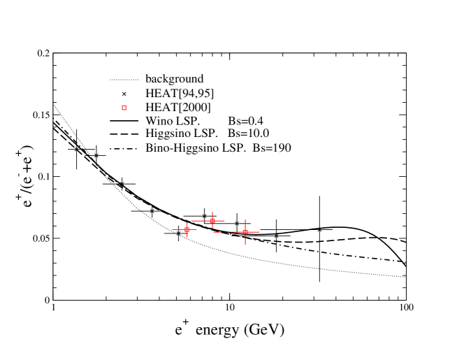
If we assume $\Omega_{\widetilde{N}_{1}}\approx 0.23$ by either thermal (for the third model) or non-thermal production (for the first two models), then there will be interesting experimental signatures. One of them is a positron excess in cosmic rays. Such an excess has been reported by the HEAT experiment[55] and two other experiments (AMS and PAMELA) [56] have been planned which will give improved results in the future. In fact the HEAT excess is currently the only reported dark matter signal that is consistent with other data. In both the wino LSP and the higgsino LSP models, LSPs annihilate to $W$ bosons quite efficiently. In particular, $W^{+}$ decays to a positron(and a neutrino). We used DARKSUSY[57] to fit the HEAT experiment measurements[58]. The fitted curves are shown in Figure 1. The “boost” factors, which characterize the local CDM density fluctuation against the averaged halo CDM density, in both models are not large. Small changes in other parameters could give boost factors very near unity. Thus both models give a nice explanation for the measured positron excess in the cosmic ray data. For the mixed LSP model, because the LSPs do not annihilate efficiently, one needs a “boost” factor of $\mathcal{O}(100)$ to get a good fit, which may be a bit too high.

Figure 1: Cosmic ray positron excess due to LSP annihilations. Crossed points are HEAT experimental data. The dotted line is from the standard cosmological model without taking into account the LSP annihilation contributions. The solid line is for the $\widetilde{W}$ LSP model, the dashed line is for the $\widetilde{H}$ LSP model and the dashed -dotted line is for the mixed $\widetilde{B}$-$\widetilde{H}$ LSP model. Bs is the boost factor.

6 Conclusion

In this paper we investigated some phenomenological implications of intersecting D-brane models, with emphasis on dark matter. We calculated the soft SUSY breaking terms in these models focussing on the $u$ moduli dominated SUSY breaking scenario in type $IIA$, in which case the results do not depend on the Yukawa couplings and Wilson lines. The results depend on the brane wrapping numbers as well as SUSY breaking parameters. Our main result is providing in detail the soft-breaking Lagrangian for intersecting brane models, which provides a new set of soft parameters to study phenomenologically. We use a rather general parameterization of F-term vevs, based on [40], which can be specialized to include the recent progress on susy breaking by flux compactification [18, 19, 20]. Our results overlap and are consistent with those of [20]. We applied our results to a particular intersecting brane model[12] which gives an MSSM-like particle spectrum, and then selected three representative points in the parameter space with relatively light gluinos, in order to reduce fine-tuning, and calculated the weak scale spectrum for them. The phenomenology of the three models corresponding to the three points is very interesting. The LSPs have different properties. They can be either wino-like, higgsino-like, or a mixture of bino and higgsino. All of them can be good candidates for the CDM.

7 Appendix

Here, we list the formulas for the soft scalar mass parameters and the trilinear parameters. It turns out that for the matter content in Table 2, we have the following independent soft parameters :

• Trilinear parameters ($A$):

  $$A_{Q_{L}H_{u}U_{R}} = \frac{-\sqrt{3}m_{3/2}}{4\pi}\,[2\pi({\Theta}_{2}+{\Theta}_{3})+[({\Theta}_{3}-{\Theta}_{2})\left(\Psi({\theta}^{2}_{ab})+\Psi({\theta}^{3}_{ab})-\Psi({\theta}^{2}_{ca})-\Psi({\theta}^{3}_{ca})\right)$$ (44)

  $$+{\Theta}_{1}\,\left(\Psi({\theta}^{2}_{ab})-\Psi({\theta}^{3}_{ab})-\Psi({\theta}^{2}_{ca})+\Psi({\theta}^{3}_{ca})\right)]\,\sin(2\pi\alpha)\,]$$

  $$A_{Q_{L}H_{d}D_{R}} = -\frac{\sqrt{3}m_{3/2}}{4\pi}\,[2\pi({\Theta}_{2}+{\Theta}_{3})+[({\Theta}_{3}-{\Theta}_{2})\left(\Psi({\theta}^{2}_{ab})+\Psi({\theta}^{3}_{ab})-\Psi({\theta}^{2}_{c*a})-\Psi({\theta}^{3}_{c*a})\right)$$ (45)

  $$+{\Theta}_{1}\,\left(\Psi({\theta}^{2}_{ab})-\Psi({\theta}^{3}_{ab})-\Psi({\theta}^{2}_{c*a})+\Psi({\theta}^{3}_{c*a})\right)]\,\sin(2\pi\alpha)\,]$$

  $$A_{Q_{L}H_{d}D_{R}} = A_{LH_{d}E_{R}};\;\;A_{Q_{L}H_{u}U_{R}}=A_{LH_{u}N_{R}}$$

• Scalar Mass parameters (${\tilde{m}}^{2}$):

  $${\tilde{m}}^{2}_{Q_{L}} = \frac{-m_{3/2}^{2}}{16{\pi}^{2}}\;[-12\pi\,\{{{\Theta}_{1}}^{2}({\Psi}({\theta}^{2}_{ab})-{\Psi}({\theta}^{3}_{ab}))-({{\Theta}_{2}}^{2}-{{\Theta}_{3}}^{2})({\Psi}({\theta}^{2}_{ab})+{\Psi}({\theta}^{3}_{ab}))\}\,\sin(2\pi\alpha)+$$ (46)

  $$3\,\{-2{\Theta}_{1}({\Theta}_{2}-{\Theta}_{3})({\Psi}^{\prime}({\theta}^{2}_{ab})-{\Psi}^{\prime}({\theta}^{3}_{ab}))+{{\Theta}_{1}}^{2}({\Psi}^{\prime}({\theta}^{2}_{ab})+{\Psi}^{\prime}({\theta}^{3}_{ab}))+$$

  $$({\Theta}_{2}-{\Theta}_{3})^{2}({\Psi}^{\prime}({\theta}^{2}_{ab})+{\Psi}^{\prime}({\theta}^{3}_{ab}))\}\,{\sin}^{2}(2\pi\alpha)+\pi\,[(-4\pi)+$$

  $$3\,\{{\Theta}_{1}^{2}({\Psi}({\theta}^{2}_{ab})-{\Psi}({\theta}^{3}_{ab}))+({\Theta}_{2}-{\Theta}_{3})^{2}({\Psi}({\theta}^{2}_{ab})-{\Psi}({\theta}^{3}_{ab}))-$$

  $$2{\Theta}_{1}({\Theta}_{2}-{\Theta}_{3})({\Psi}({\theta}^{2}_{ab})+{\Psi}({\theta}^{3}_{ab}))\}\,\sin(4\pi\alpha)\,]\;]$$

  $${\tilde{m}}^{2}_{U_{R}} = \frac{-m_{3/2}^{2}}{16{\pi}^{2}}\;[-12\pi\,\{{{\Theta}_{1}}^{2}({\Psi}({\theta}^{2}_{ac})-{\Psi}({\theta}^{3}_{ac}))-({{\Theta}_{2}}^{2}-{{\Theta}_{3}}^{2})({\Psi}({\theta}^{2}_{ac})+{\Psi}({\theta}^{3}_{ac}))\}\,\sin(2\pi\alpha)+$$ (47)

  $$3\,\{-2{\Theta}_{1}({\Theta}_{2}-{\Theta}_{3})({\Psi}^{\prime}({\theta}^{2}_{ac})-{\Psi}^{\prime}({\theta}^{3}_{ac}))+{{\Theta}_{1}}^{2}({\Psi}^{\prime}({\theta}^{2}_{ac})+{\Psi}^{\prime}({\theta}^{3}_{ac}))+$$

  $$({\Theta}_{2}-{\Theta}_{3})^{2}({\Psi}^{\prime}({\theta}^{2}_{ac})+{\Psi}^{\prime}({\theta}^{3}_{ac}))\}\,{\sin}^{2}(2\pi\alpha)+\pi\,[(-4\pi)+$$

  $$3\,\{{\Theta}_{1}^{2}({\Psi}({\theta}^{2}_{ac})-{\Psi}({\theta}^{3}_{ac}))+({\Theta}_{2}-{\Theta}_{3})^{2}({\Psi}({\theta}^{2}_{ac})-{\Psi}({\theta}^{3}_{ac}))-$$

  $$2{\Theta}_{1}({\Theta}_{2}-{\Theta}_{3})({\Psi}({\theta}^{2}_{ac})+{\Psi}({\theta}^{3}_{ac}))\}\,\sin(4\pi\alpha)\,]\;]$$

  $${\tilde{m}}^{2}_{D_{R}} = \frac{-m_{3/2}^{2}}{16{\pi}^{2}}\;[-12\pi\,\{{{\Theta}_{1}}^{2}({\Psi}({\theta}^{2}_{ac*})-{\Psi}({\theta}^{3}_{ac*}))-({{\Theta}_{2}}^{2}-{{\Theta}_{3}}^{2})({\Psi}({\theta}^{2}_{ac*})+{\Psi}({\theta}^{3}_{ac*}))\}\,\sin(2\pi\alpha)+$$ (48)

  $$3\,\{-2{\Theta}_{1}({\Theta}_{2}-{\Theta}_{3})({\Psi}^{\prime}({\theta}^{2}_{ac*})-{\Psi}^{\prime}({\theta}^{3}_{ac*}))+{{\Theta}_{1}}^{2}({\Psi}^{\prime}({\theta}^{2}_{ac*})+{\Psi}^{\prime}({\theta}^{3}_{ac*}))+$$

  $$({\Theta}_{2}-{\Theta}_{3})^{2}({\Psi}^{\prime}({\theta}^{2}_{ac*})+{\Psi}^{\prime}({\theta}^{3}_{ac*}))\}\,{\sin}^{2}(2\pi\alpha)+\pi\,[(-4\pi)+$$

  $$3\,\{{\Theta}_{1}^{2}({\Psi}({\theta}^{2}_{ac*})-{\Psi}({\theta}^{3}_{ac*}))+({\Theta}_{2}-{\Theta}_{3})^{2}({\Psi}({\theta}^{2}_{ac*})-{\Psi}({\theta}^{3}_{ac*}))-$$

  $$2{\Theta}_{1}({\Theta}_{2}-{\Theta}_{3})({\Psi}({\theta}^{2}_{ac*})+{\Psi}({\theta}^{3}_{ac*}))\}\,\sin(4\pi\alpha)\,]\;]$$

  $${\tilde{m}}^{2}_{Q_{L}} = {\tilde{m}}^{2}_{L};\;\;{\tilde{m}}^{2}_{U_{R}}={\tilde{m}}^{2}_{N_{R}};\;\;{\tilde{m}}^{2}_{D_{R}}={\tilde{m}}^{2}_{E_{R}}$$

The above formulas are subject to the constraint $|{\Theta}_{1}|^{2}+|{\Theta}_{2}|^{2}+|{\Theta}_{3}|^{2}=1$, as can be seen below (24).

Acknowledgement
The authors appreciate helpful conversations with and suggestions from Brent D. Nelson,
Andrew Pawl and Lian-Tao Wang. The research of GLK, PK, JDL and TTW are supported in part by the US Department of Energy.