Abstract

In the framework of the $k_{T}$-factorization approach we have calculated in the fragmentation model the $p_{T}$-spectra of $B_{c}$ mesons at the energies of the Tevatron and the LHC Colliders and at the large $p_{T}$ domain. We compare the obtained results with the existing experimental data and with the predictions obtained in the collinear parton model.

1 Introduction

Recently, $B_{c}$ mesons were observed experimentally [1, 2]. These particles have a special place in the doubly heavy meson family, because they consist of quarks of different flavors. The $B_{c}$ meson spectroscopy has the same features as the spectroscopies of charmonia and bottomonia, however the decay and production properties of $B_{c}$ mesons are unique. There is no annihilation channel for $B_{c}$ mesons into hadrons via the gluons and, consequently, the lifetime of the ground state of the $\bar{b}c$ system is large, given by $\tau\approx 0.46$ ps [2]. The main channel of $B_{c}$ meson decay occurs through the weak decays of the $b$-quark or the $c$-quark, which are respectively about 25% and 65% of the total decay width.

The $B_{c}$ meson hadroproduction cross section is approximately 100 times smaller than the ($b\bar{b}$)-pair production cross section, because the two pairs of the heavy quarks are produced in a parton subprocess. The mass spectrum and the decay properties of the $B_{c}$ mesons are studied in detail in the framework of potential quark models [3], in the QCD sum rules methods [4] and in the OPE approach [5]. The predictions at leading order in $\alpha_{s}$ for the $B_{c}$ meson production rates in the $\gamma\gamma$, $\gamma p$ and $pp$ interactions were obtained in the collinear parton model [6, 7, 8, 9, 10].

The $B_{c}$ meson production cross section became large enough to study experimental ($\sim 1$ nb) only in the region of very high energy or in the region of very small $x\sim M/\sqrt{s}\sim 10^{-2}$, where $x$ is the argument of the gluon distribution function in a proton (the quark contribution to the hadronic production of $B_{c}$ mesons is very small). In this region the $k_{T}$-factorization approach [11, 12] is more adequate for describing the perturbative evolution of the gluon distribution function, which satisfies the BFKL [13] or CCFM [14] evolution equations, in comparison with the collinear parton model, which is based on the DGLAP equation [15].

In this Latter we have calculated $B_{c}$ meson $p_{T}$-spectra at the energy range of the Tevatron and the LHC Colliders in the fragmentation model and in the framework of the $k_{T}$-factorization approach. In the fragmentation model we have taken into consideration only the main contribution originating from fragmentation of a b-quark into a $B_{c}$ meson [16].

2 The $k_{T}$-factorization approach

In the $k_{T}$-factorization approach [11, 12], which generalizes the collinear parton model to the region of small $x$, the hadronic and partonic cross sections are related as follows:

$$\sigma^{\mathrm{KT}}(p\bar{p}\to b\bar{b}X,s)=\int{\frac{dx_{1}}{x_{1}}}\int{d|\vec{k}_{1T}|^{2}}\int{\frac{d\varphi_{1}}{2\pi}}\Phi(x_{1},|\vec{k}_{1T}|^{2},\mu^{2})\times$$

$$\times\int{\frac{dx_{2}}{x_{2}}}\int{d|\vec{k}_{2T}|^{2}}\int{\frac{d\varphi_{2}}{2\pi}}\Phi(x_{2},|\vec{k}_{2T}|^{2},\mu^{2})\hat{\sigma}(g^{\star}g^{\star}\to b\bar{b},\hat{s})\mbox{,}$$ (1)

where $\Phi(x,|\vec{k}_{T}|^{2},\mu^{2})$ is the unintegrated gluon distribution function in a proton (unintegrated refers to the transverse momentum), $|{\vec{k}}_{i,T}|^{2}$ is the virtuality of the initial reggeized gluon, $k_{i}=x_{i}p_{i}+k_{i,T}$ is the 4-momentum of the initial gluon, $k_{i,T}=(0,\vec{k}_{i,T},0)$ is the transverse momentum of the initial gluon, $\varphi_{i}$ is the angle between the gluon transverse momentum and the fixed axis $OX$ in the plane $XOY$, $\hat{s}=x_{1}x_{2}s-|\vec{k}_{1T}|^{2}-|\vec{k}_{2T}|^{2}$. In the numerical calculations we have used the following parameterizations for the unintegrated gluon distribution function in a proton: JB by Blumlein [17], JS by Jung and Salam [18] and KMR by Kimber, Martin and Ryskin [19].

To calculate the amplitude of partonic processes in the $k_{T}$-factorization approach the polarization vector for the reggeized gluon in the initial state is taken to be [11, 12]

$$\varepsilon^{\mu}(k_{T})=\frac{k_{T}^{\mu}}{|\vec{k}_{T}|}\mbox{.}$$ (2)

The squared amplitude for one of the processes in $B_{c}$ meson production in the $k_{T}$-factorization approach, namely

$$g^{\star}+g^{\star}\to b+\bar{b}$$ (3)

was obtained earlier in [11]. Here we use our original results from Ref. [20]

$$\overline{|M(g^{\star}+g^{\star}\to Q+\bar{Q})|^{2}}=8\pi^{2}\alpha_{s}^{2}(M_{11}+M_{22}+M_{33}+2M_{12}+2M_{13}+2M_{23})\mbox{,}$$ (4)

where

$$M_{11} = \frac{1}{3{\tilde{t}}^{2}}\Bigl{(}\kappa_{1}(4\beta_{1}-\kappa_{1})(\kappa_{1}^{2}+\kappa_{2}^{2}-4\beta_{2}\kappa_{2})+4\lambda\beta_{2}(\kappa_{1}-2\beta_{1})(4\kappa_{2}^{2}+{\tilde{t}})+4\kappa_{1}^{3}(\lambda\kappa_{2}-\beta_{1})$$ (5)

$$+ 4\beta_{2}^{2}(\kappa_{1}^{2}+4\beta_{1}\kappa_{1}-4\lambda\kappa_{1}\kappa_{2})+4\lambda\kappa_{2}(\lambda\kappa_{2}-2\beta_{1})(\kappa_{1}^{2}-4\beta_{2}^{2})-4\beta_{1}^{2}(2\beta_{2}-\kappa_{2})^{2}+\kappa_{1}^{4}$$

$$+ 4\lambda\kappa_{2}(2\lambda\beta_{2}+\beta_{1})(2\kappa_{2}^{2}+{\tilde{t}})+8\lambda\beta_{1}\kappa_{2}^{3}+4\lambda\kappa_{2}({\hat{s}}+{\tilde{u}})(\kappa_{1}+\lambda\kappa_{2})+{\tilde{t}}{\tilde{u}}\Bigr{)}\mbox{,}$$

$$M_{22} = \frac{1}{3{\tilde{u}}^{2}}\Bigl{(}\kappa_{2}^{4}-4\beta_{2}\kappa_{2}^{3}-4\beta_{2}^{2}(\kappa_{1}^{2}+\kappa_{2}^{2})+16\beta_{1}\beta_{2}^{2}(\kappa_{1}-\beta_{1})+4\lambda\bigl{(}4\beta_{1}\kappa_{1}^{2}(\kappa_{2}-2\beta_{2})+{\tilde{t}}{\tilde{u}}$$ (6)

$$+ \kappa_{1}(\kappa_{2}^{3}-2\beta_{2}\kappa_{2}^{2}+(\kappa_{2}-\beta_{2})({\hat{s}}+{\tilde{t}}-4\beta_{1}^{2})-\beta_{2}{\tilde{u}})-\beta_{1}(2\beta_{2}-\kappa_{2}){\tilde{u}}\bigr{)}-16\lambda^{2}\beta_{1}^{2}\kappa_{1}^{2}$$

$$+ 4\lambda^{2}\kappa_{1}(4\beta_{1}\kappa_{1}^{2}-\kappa_{1}(\kappa_{1}^{2}+{\tilde{u}})+2\beta_{1}{\tilde{u}})+\kappa_{2}(4\beta_{2}-\kappa_{2})((2\beta_{1}^{2}-\kappa_{1})^{2}+\kappa_{2}^{2})+4\kappa_{2}^{2}\beta_{2}^{2}\Bigr{)}\mbox{,}$$

$$M_{33} = \frac{3}{4{\hat{s}}^{2}}\Bigl{(}(\kappa_{1}^{2}+\kappa_{2}^{2}){\hat{s}}-4(\beta_{2}\kappa_{1}-\beta_{1}\kappa_{2})^{2}+4\lambda\beta_{1}\kappa_{2}(\kappa_{1}^{2}-\kappa_{2}^{2}-{\hat{t}}+{\hat{u}})$$ (7)

$$- \lambda^{2}\bigl{(}\kappa_{1}^{4}+\kappa_{2}^{4}-8\beta_{1}\kappa_{1}^{3}-8\beta_{2}\kappa_{2}^{3}-{\hat{s}}^{2}+{\hat{t}}^{2}+8\beta_{1}\kappa_{1}(\kappa_{2}^{2}-4\beta_{2}\kappa_{2}+{\hat{t}}-{\hat{u}})-2{\hat{t}}{\hat{u}}+{\hat{u}}^{2}$$

$$- 2\kappa_{1}^{2}(\kappa_{2}^{2}-4\beta_{2}\kappa_{2}-8\beta_{1}^{2}+{\hat{t}}-{\hat{u}})+2\kappa_{2}^{2}(8\beta_{2}^{2}+{\hat{t}}-{\hat{u}})-8\beta_{2}\kappa_{2}({\hat{t}}-{\hat{u}})\bigr{)}$$

$$- 2\lambda\bigl{(}8\beta_{2}^{2}\kappa_{1}\kappa_{2}+2\beta_{2}(\kappa_{1}^{3}-4\beta_{1}\kappa_{1}^{2}-4\beta_{1}\kappa_{2}^{2}-\kappa_{1}(\kappa_{2}^{2}+{\hat{t}}-{\hat{u}}))+\kappa_{1}\kappa_{2}(8\beta_{1}^{2}-{\hat{s}})\bigr{)}\Bigr{)}\mbox{,}$$

$$M_{12} = -\frac{1}{48{\tilde{t}}{\tilde{u}}}\biggl{(}4\beta_{1}\kappa_{1}^{3}+\kappa_{2}^{2}({\hat{s}}-8\beta_{1}^{2}-{\tilde{t}}-{\tilde{u}})+32\beta_{1}\beta_{2}(\beta_{1}\kappa_{2}-\beta_{1}\beta_{2})+{\hat{s}}^{2}-{\tilde{t}}^{2}-{\tilde{u}}^{2}$$ (8)

$$- \kappa_{1}^{2}(\kappa_{2}^{2}-\kappa_{1}^{2}-8\beta_{2}\kappa_{2}+8\beta_{2}^{2}-2{\hat{s}})+4\beta_{1}\kappa_{1}(2\kappa_{2}^{2}-8\beta_{2}\kappa_{2}+8\beta_{2}^{2}-\kappa_{1}^{2})+2\lambda^{2}\Bigl{(}\kappa_{1}^{4}$$

$$+ \kappa_{2}^{4}-{\hat{s}}^{2}+{\tilde{t}}^{2}+{\tilde{u}}^{2}+4\beta_{2}\kappa_{2}{\tilde{u}}+2\kappa_{2}^{2}{\tilde{t}}+2\kappa_{1}^{2}(4\beta_{2}\kappa_{2}+{\tilde{u}})+4\beta_{1}\kappa_{1}(2\kappa_{2}^{2}-4\beta_{2}\kappa_{2}$$

$$+ {\tilde{t}})\Bigr{)}-4\lambda\Bigl{(}4\beta_{2}^{2}\kappa_{2}(\kappa_{1}-2\beta_{1})-\kappa_{2}(-4\beta_{1}^{2}\kappa_{1}+\beta_{1}(3\kappa_{1}^{2}+\kappa_{2}^{2}-{\hat{s}})+\kappa_{1}{\hat{s}})-\beta_{2}\bigl{(}\kappa_{1}^{3}$$

$$- 4\beta_{1}\kappa_{1}^{2}+\kappa_{1}(3\kappa_{2}^{2}+8\beta_{1}^{2}-{\hat{s}})+2\beta_{1}({\hat{s}}-3\kappa_{2}^{2}-\kappa_{1}^{2})\bigr{)}\Bigr{)}\biggr{)}\mbox{,}$$

$$M_{13} = -\frac{3}{16{\hat{s}}{\tilde{t}}}\biggl{(}2(\lambda^{2}-1)\kappa_{1}^{4}+2\kappa_{1}^{3}(2\beta_{1}-\lambda\kappa_{2}-3\beta_{1}\lambda^{2}+3\lambda\beta_{2})+2\beta_{1}\lambda(2\kappa_{2}^{3}+4\beta_{2}\kappa_{2}^{2}$$ (9)

$$+ 4\beta_{2}({\hat{t}}-{\hat{u}})-\kappa_{2}(16\beta_{2}^{2}-2{\tilde{u}}))-\kappa_{1}^{2}(2(1+\lambda^{2})\kappa_{2}^{2}-2((5\lambda^{2}-2)\beta_{2}+6\beta_{1}\lambda)\kappa_{2}$$

$$+ 24\lambda\beta_{1}\beta_{2}-8\beta_{2}^{2}+2{\hat{s}}-\lambda^{2}{\hat{s}}+\lambda^{2}{\tilde{t}}+2{\tilde{u}}-3\lambda^{2}{\tilde{u}})+2\kappa_{2}\beta_{2}(8\beta_{1}^{2}+{\tilde{t}}+{\tilde{u}})-4\beta_{1}^{2}\kappa_{2}$$

$$- \kappa_{2}{\tilde{u}}+\lambda^{2}(4\kappa_{2}^{4}-22\beta_{2}\kappa_{2}^{3}-{\hat{s}}^{2}+({\hat{t}}-{\hat{u}})^{2}-\kappa_{2}^{2}({\hat{s}}-32\beta_{2}^{2}-5{\tilde{t}}+3{\tilde{u}})+2\beta_{2}\kappa_{2}({\hat{s}}$$

$$- 7{\tilde{t}}+5{\tilde{u}}))+2\kappa_{1}(\beta_{1}\lambda^{2}(5\kappa_{2}^{2}-16\beta_{2}\kappa_{2}-3{\hat{s}}+{\tilde{t}}-3{\tilde{u}})+\beta_{1}(4\kappa_{2}^{2}-8\beta_{2}^{2}+2{\hat{s}}+{\tilde{t}}$$

$$+ {\tilde{u}})+\lambda(3\kappa_{2}^{3}-11\beta_{2}\kappa_{2}^{2}+\kappa_{2}(16\beta_{2}^{2}-8\beta_{1}^{2}+2{\tilde{t}}-{\tilde{u}})+\beta_{2}(16\beta_{1}^{2}+{\hat{s}}-3{\hat{t}}+3{\hat{u}})))\biggr{)}\mbox{,}$$

$$M_{23} = -\frac{3}{16{\hat{s}}{\tilde{u}}}\biggl{(}\lambda^{2}(4\kappa_{1}^{4}+2\kappa_{2}^{4}-22\beta_{1}\kappa_{1}^{3}-{\hat{s}}^{2}+2\beta_{1}\kappa_{1}(5\kappa_{2}^{2}-16\beta_{2}\kappa_{2}+{\hat{s}}+5{\tilde{t}}-7{\tilde{u}})$$ (10)

$$- \kappa_{1}^{2}(2\kappa_{2}^{2}-16\beta_{2}\kappa_{2}-32\beta_{1}^{2}+{\hat{s}}+3{\tilde{t}}-5{\tilde{u}})+\kappa_{2}^{2}({\hat{s}}+3{\tilde{t}}-{\tilde{u}})+({\hat{t}}-{\hat{u}})^{2}+8\beta_{2}\kappa_{2}{\tilde{u}})$$

$$- 2(\kappa_{1}^{2}(\kappa_{2}^{2}-3\beta_{2}\kappa_{2}+4\beta_{2}^{2}+{\tilde{t}})+\kappa_{2}(\kappa_{2}^{3}-\beta_{2}\kappa_{2}^{2}+\kappa_{2}({\hat{s}}-4\beta_{1}^{2}+{\tilde{t}})+\beta_{2}(8\beta_{1}^{2}-{\hat{s}}))$$

$$- \beta_{1}\kappa_{1}(8\beta_{2}^{2}-2\kappa_{2}^{2}+{\tilde{t}}+{\tilde{u}}))+2\lambda(\kappa_{1}^{3}(\kappa_{2}+2\beta_{2})+\beta_{1}\kappa_{1}^{2}(4\beta_{2}-11\kappa_{2})+\beta_{1}(4\beta_{2}({\hat{u}}-{\hat{t}})$$

$$+ 3\kappa_{2}^{3}-12\beta_{2}\kappa_{2}^{2}+\kappa_{2}(16\beta_{2}^{2}+{\hat{s}}+3{\hat{t}}-3{\hat{u}}))-\kappa_{1}(3\kappa_{2}^{3}-8\beta_{2}\kappa_{2}^{2}-\kappa_{2}(16\beta_{1}^{2}-8\beta_{2}^{2}-2{\hat{s}}$$

$$- 3{\tilde{t}}+{\tilde{u}})+\beta_{2}(16\beta_{1}^{2}-{\tilde{t}})))\biggr{)}\mbox{,}$$

where

$${\tilde{t}} = {\hat{t}}-m_{Q}^{2}\mbox{,}$$ (11)

$${\tilde{u}} = {\hat{u}}-m_{Q}^{2}\mbox{,}$$ (12)

$$\beta_{1} = |{\vec{p}}_{T}|\cos{\varphi_{1}}\mbox{,}$$ (13)

$$\beta_{2} = |{\vec{p}}_{T}|\cos{\varphi_{2}}\mbox{,}$$ (14)

$$\kappa_{1} = |{\vec{k}}_{1T}|\mbox{,}$$ (15)

$$\kappa_{2} = |{\vec{k}}_{2T}|\mbox{,}$$ (16)

$$\lambda = \cos{(\varphi_{1}-\varphi_{2})}$$ (17)

and ${\vec{p}}_{T}$ — transverse momentum of anti-quark. Since these are more suitable for numerical calculations. In those calculations, which were in the framework of the collinear parton model, we used the GRV [21] parameterization for the gluon distribution function.

3 The fragmentation model

The analysis of the $B_{c}$ meson gluon-gluon production in the framework of the collinear parton model shows [6, 7, 8] the dominant role of the fusion mechanism up to $p_{T}\thickapprox 30$ GeV. It takes into account the total gauge invariant set of the diagrams which describes the parton process

$$g+g\to B_{c}+b+\bar{c}\mbox{.}$$ (18)

Thus, the fragmentation approximation, incorporating factorization of the heavy quark production process and the soft process of a meson created in the final state, applies only at $p_{T}>30$ GeV. Of course, at the Tevatron Collider this region of $p_{T}$ is far from being available for experimental study. On the other hand, at the LHC Collider the $p_{T}\leq 50$ GeV region will be under consideration.

In the fragmentation model, the $B_{c}$ meson production cross section can be presented as follows:

$$d\sigma(pp\to B_{c}X)=\sum_{i}\int{dz}D_{i\to B_{c}}(z)\cdot d\hat{\sigma}(pp\to i)\mbox{,}$$ (19)

where the sum is taken over all the relevant partons $i=c$, $b$ and $g$ (but the main contribution comes from $b$-quark fragmentation).

The fragmentation functions for the $b$-quark splitting into a vector $B_{c}^{*}$ and pseudoscalar $B_{c}$ meson at the starting scale of the perturbative QCD evolution were obtained in Ref. [22, 23]:

$$D_{\bar{b}\to B_{c}}(z,\mu_{0}) = \frac{8\alpha_{s}^{2}(\mu_{0})|\Psi_{B_{c}}(0)|^{2}}{81m_{c}^{3}}\frac{r(1-z)^{2}z}{(1-(1-r)z)^{6}}\Bigl{(}6-18(1-2r)z+(21-74r+68r^{2})z^{2}$$ (20)

$$- 2(1-r)(6-19r+18r^{2})z^{3}+3(1-r)^{2}(1-2r+2r^{2})z^{4}\Bigr{)}\mbox{,}$$

$$D_{\bar{b}\to B_{c}^{\star}}(z,\mu_{0}) = \frac{8\alpha_{s}^{2}(\mu_{0})|\Psi_{B_{c}}(0)|^{2}}{27m_{c}^{3}}\frac{r(1-z)^{2}z}{(1-(1-r)z)^{6}}\Bigl{(}2-2(3-2r)z+3(3-2r+4r^{2})z^{2}$$ (21)

$$- 2(1-r)(4-r+2r^{2})z^{3}+(1-r)^{2}(3-2r+2r^{2})z^{4}\Bigr{)}\mbox{,}$$

where $r=\frac{m_{c}}{m_{c}+m_{b}}$. $|\Psi_{B_{c}}(0)|^{2}$ is the squared $B_{c}$ meson wave function at the origin, which can be calculated using the nonrelativistic potential quark model [24]. In the numerical calculations, we used the result $\Psi_{B_{c}}(0)=\sqrt{\frac{m_{B_{c}}}{12}}f_{B_{c}}$, where $f_{B_{c}}=490-560$ MeV is the $B_{c}$ meson leptonic decay constant.

The QCD evolution of the fragmentation functions $D_{\bar{b}\to B_{c}}$ and $D_{\bar{b}\to B_{c}^{\star}}$ are described by the DGLAP [15] evolution equation

$$\mu^{2}\frac{\partial D}{\partial\mu^{2}}(z,\mu^{2})=\frac{\alpha_{s}(\mu^{2})}{2\pi}\int_{z}^{1}\frac{dx}{x}P_{q\to q}(\frac{x}{z})D(x,\mu^{2})\mbox{,}$$ (22)

where $P_{q\to q}(z)$ is the standard quark-quark splitting function.

4 The results

The results of our calculation for the $p_{T}$-spectra of the $B_{c}^{\star}$ meson are shown in Fig. 1 for the energy of the Tevatron Collider $\sqrt{s}=1.8$ TeV, and in the Fig. 2 for the energy of the LHC Collider $\sqrt{s}=14$ TeV. The spectra that we obtain are compared with those obtained earlier in the collinear parton model via the fragmentation mechanism. The curves in Fig. 1 correspond to a choice of the parameters from Ref. [16]: $m_{c}=1.5$ GeV, $m_{b}=4.9$ GeV, $\alpha_{s}=\alpha_{s}(p_{T}^{2}+m_{B_{c}}^{2})$ and $f_{B_{c}}=490$ MeV. The curves in Fig. 2 were obtained using the set of parameters from Ref. [6]: $m_{c}=1.5$ GeV, $m_{b}=5.1$ MeV, $\alpha_{s}\simeq 0.23$ and $f_{B_{c}}=560$ MeV.

Fig. 1 shows that our result obtained in the collinear parton model agrees well with the result obtained earlier in Ref. [16]. The curves obtained in the $k_{T}$-factorization approach lie approximately 2—5 times higher than the collinear parton model prediction in the region $p_{T}>10$ GeV. The maximum value of the $B_{c}$ meson production cross section is obtained using the JS [18] parameterization of the unintegrated gluon distribution function, and the minimum value is obtained using the JB [17] parameterization.

Note that the slopes of the $p_{T}$-spectra obtained in the collinear parton model and in the $k_{T}$-factorization approach are equal, and the situation is the same as in the case of $D^{\star}$ meson production in $ep$ interactions [25, 26].

At present, there is no experimental information on the $p_{T}$-spectra of $B_{c}$ mesons. It is known that the integrated production cross section in the region $p_{T}>6$ GeV, $|y|<1$ and $\sqrt{s}=1.8$ TeV is given by $\sigma_{B_{c}}\simeq 10\pm 6$ nb [1, 2]. As shown in Ref. [6], the uncertainties in the calculations are about $\sim 50$%. This value depends on the choice of the masses, the $\alpha_{s}$ constant and the leptonic decay constant $f_{B_{c}}$. Furthermore, our calculations performed in the $k_{T}$-factorization approach show that the $B_{c}$ meson production cross section has a strong dependence on the choice of the unintegrated gluon distribution function — a variation by a factor of 2 was observed.

The obtained values of the integrated $B_{c}$ and $B_{c}^{\star}$ meson production cross section at the energies of the Tevatron and the LHC Colliders are presented in Table 1. One can see that, with the fragmentation model, the results obtained in the collinear parton model are smaller to those obtained in the $k_{T}$-factorization approach. The theoretical predictions are shown together with their uncertainties, which are significantly larger in the $k_{T}$-factorization approach. The absolute value of the cross section obtained in the collinear parton model ($\sigma_{B_{c}}=1.7\pm 0.8$ nb) is much smaller than the CDF experimental data ($\sigma_{B_{c}}=10\pm 6$ nb) [1, 2]. On the other hand, the prediction of the $k_{T}$-factorization approach agrees well with the data ($\sigma_{B_{c}}=7.4\pm 5.4$ nb).

Taking into account the relative roles of the fusion and fragmentation mechanisms in $B_{c}$ meson hadroproduction, one can suppose that the cross section calculated in the fusion model and in the $k_{T}$-factorization approach will be more large than that obtained in the fragmentation model and in the $k_{T}$-factorization approach. The calculation of the $B_{c}$ meson hadroproduction rates via the partonic subprocess (18) with the reggeized initial gluons will be presented in our forthcoming paper.

5 Acknowledgments

We thank B. Kniehl and A. Likhoded for useful discussions about the results obtained. The work is supported by the Russian Federal Agency of Education under Grant A04-2.9-52. The part of the D.V. work was done in the framework of the Grant ”Mikhail Lomonosov”, which is supported by DAAD and by Russian Ministry of Education. D.V. thanks the International Center of Fundamental Physics in Moscow and Dynastiya Foundation for the financial support received while this work was done.

Table 1: The summed $B_{c}$ and $B_{c}^{\star}$ meson production cross sections in the different models at the energies of the Tevatron and LHC Colliders. The data from the CDF Collaboration[1, 2] are shown. The cross sections are in nb.

$\sqrt{s},$	$|y|$	$p_{T,min}$,	Parton	$k_{T}$-factorization	Experimental
TeV		GeV	model	approach	data
$1.8$	$<1$	$6$	$1.7\pm 0.8$	$7.4\pm 5.4$	$10\pm 6$
$14$	$<2.5$	$10$	$28\pm 14$	$122\pm 90$	—

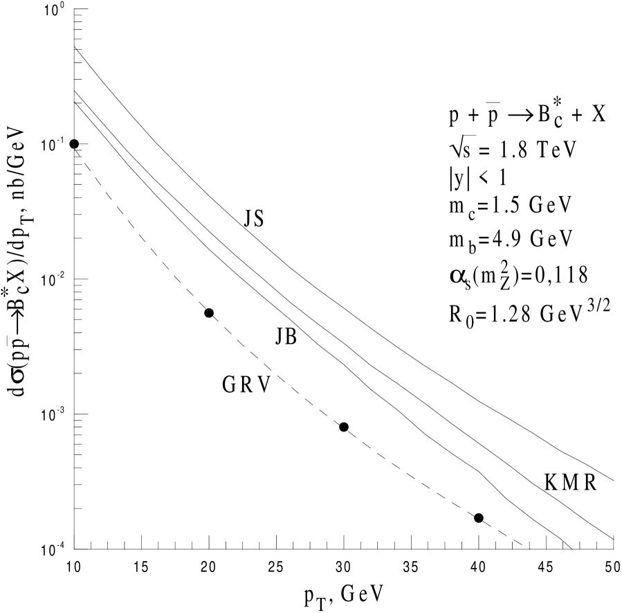
Figure 1: The $B_{c}^{\star}$ meson $p_{T}$-spectrum at $\sqrt{s}=1.8$ TeV and $|y|<1$ in the fragmentation model. The continuous lines are a result of calculations in the $k_{T}$-factorization approach with the different parameterizations of the unintegrated gluon distribution function. The dashed line is the prediction from the collinear parton model. The points show the results obtained in the Ref. [16].

Figure 2: The $B_{c}^{\star}$ meson $p_{T}$-spectrum at $\sqrt{s}=14$ TeV and $|y|<2.5$ in the fragmentation model. The continuous lines are results of calculations in the $k_{T}$-factorization approach with the different parameterizations of the unintegrated gluon distribution function. The dashed line is the prediction from the collinear parton model.

References

- [1] CDF Collaboration, F. Abe, at al., Phys. Rev. Lett. 81 (1998) 2432; CDF Collaboration, F. Abe, at al., Phys. Rev. D 58 (1998) 112004.
- [2] K. Anikeev, at al., FERMILAB-Pub-01/197 (2001) 480.
- [3] S.S. Gershtein, V.V. Kiselev, A.K. Likhoded, S.R. Slabospitsky, A.V. Tkabladze, Yad. Fiz. 48 (1988) 515; Y.-Q. Chen, Y.-P. Kuang, Phys. Rev. D 46 (1992) 1165; E. Eichten, F. Feinberg, Phys. Rev. D 23 (1981) 2724.
- [4] V.V. Kiselev, A.K. Likhoded, A.O. Onishenko, Nucl. Phys. B 569 (2000) 473; V.V. Kiselev, A.K. Likhoded, A.E. Kovalsky, Nucl. Phys. B 585 (2000) 353.
- [5] I. Bigi, Phys. Lett. B 371 (1996) 103; M. Beneke, G. Buchalla, Phys. Rev. D 53 (1996) 4991.
- [6] A.V. Berezhnoy, A.K. Likhoded, M.V. Shevlyagin, Yad. Fiz. 58 (1995) 730; A.V. Berezhnoy, A.K. Likhoded, O.O. Yushenko, Yad. Fiz. 59 (1996) 742; A.V. Berezhnoy, V.V. Kiselev, A.K. Likhoded, Z. Phys. A 356 (1996) 79.
- [7] K. Kolodziej, R. Rückl, Nucl. Instrum. Methods A 408 (1998) 33; K. Kolodziej, A. Leike, R. Rückl, Phys. Lett. B 355 (1995) 337.
- [8] C.-H. Chang, at al., Phys. Lett. B 364 (1995) 78; C.-H. Chang, Y.-Q. Chen, R.J. Oakes, Phys. Rev. D 54 (1996) 4344.
- [9] S.P. Baranov, Phys. Rev. D 56 (1997) 3046.
- [10] A.P. Martynenko, V.A. Saleev, Phys. Rev. D 54 (1996) 1891; A.P. Martynenko, V.A. Saleev, Yad. Fiz. 59 (1996) 747.
- [11] J.C. Collins, R.K. Ellis, Nucl. Phys. 360 (1991) 3.
- [12] L.V. Gribov, E.M. Levin, M.G. Ryskin, Phys. Rep. 100 (1983) 1; S. Catani, M. Ciafoloni, F. Hautmann, Nucl. Phys. B 366 (1991) 135; V.S. Fadin, L.N. Lipatov, Nucl. Phys. B 477 (1996) 767.
- [13] E.A. Kuraev, L.N. Lipatov, V.S. Fadin, Sov. Phys. JETP 44 (1976) 443; I.I. Balitsky, L.N. Lipatov, Sov. J. Nucl. Phys. 28 (1978) 822.
- [14] M. Ciafaloni, Nucl. Phys. B 296 (1988) 49; S. Catani, F. Fiorani, G. Marchesini, Phys. Lett. B 234 (1990) 339; G. Marchesini, Nucl. Phys. B 445 (1995) 49.
- [15] V.N. Gribov, L.N. Lipatov, Sov. J. Nucl. Phys. 15 (1972) 438; Y.L. Dokshitzer, Sov. Phys. JETP 46 (1977) 641; G. Altarelli, G. Parisi, Nucl. Phys. B 126 (1977) 298.
- [16] K. Cheung, T.C. Yuan, Phys. Rev. D 53 (1996) 1232; K. Cheung, Phys. Rev. Lett. 71 (1993) 3413.
- [17] J. Blumlein, DESY 95-121 (1995).
- [18] H. Jung, G. Salam, Eur. Phys. J. C 19 (2001) 351.
- [19] M.A. Kimber, A.D. Martin, M.G. Ryskin, Phys. Rev. D 63 (2001) 114027.
- [20] V.A. Saleev, D.V. Vasin, Yad. Fiz. (2005) to be published.
- [21] M. Gluck, E. Reya, A. Vogt, Z. Phys. C 67 (1995) 433.
- [22] E. Braaten, K. Cheung, T.C. Yuan, Phys. Rev. D 48 (1993) 5049.
- [23] V.V Kiselev, A.K. Likhoded, M.V. Shevlyagin, Z. Phys. C 63 (1994) 77.
- [24] E.J. Eichten, C. Quigg, Phys. Rev. D 52 (1995) 1726.
- [25] V.A. Saleev, D.V. Vasin, Phys. Lett. B 548 (2002) 161; erratum ibid., hep-ph /0209220, v. 2.
- [26] S.P. Baranov, H. Jung, L. Jonsson, S. Padhi, N. P. Zotov, Eur. Phys. J. C 24 (2002) 425; S.P. Baranov, H. Jung, N.P. Zotov, Nucl. Phys. A (Proc. Suppl.) 99 (2001) 192.