Abstract

A complete study of the processes $B\to{\pi}^{+}{\pi}^{-}V\ \ (V=1^{--})$ is performed both in the framework of the helicity formalism and the effective lagrangian approach. Emphasis is put on the factorization hypothesis and the importance of the ${{\rho}^{0}}-{\omega}$ mixing in enhancing the direct $CP$ violation. New results involving some branching ratios and the ratio of the Penguin/Tree amplitude are given in details.

1 Physical Motivations for the channels $B\to V_{1}V_{2}$ and their Decay Kinematics

In the framework of the LHCb experiment devoted to the search for $CP$ violation and rare $B$ decays, special care is given to the $B$ decays into two vector mesons, $B\to V_{1}V_{2},\ \ V_{i}=\ 1^{--}$.

(i) $B$ decays being governed by weak interactions, the vector-mesons are polarized and their final states have specific angular distributions; which allows one to cross-check the Standard Model (SM) predictions and to perform tests of models beyond the SM.
(ii) In the special case of two neutral vector mesons with ${\bar{V}}^{0}=V^{0}\$; orbital angular momentum $\ell$, total spin $S$ and $CP$ eigenvalues are related by the following relations : $\ell=\ S\ =\ 0,1,2\ \Longrightarrow CP\ =\ {(-1)}^{\ell}\$ , which implies a mixing of different $CP$ eigenstates, proving a $CP$ non-conservation process. According to Dunietz et al [1], tests of $CP$ violation in a model independent way can be performed and severe constraints on models beyond the SM can be set. Because the $B$ meson has spin $0$, the final two vector mesons, $V_{1}$ and $V_{2}$, have the same helicity ${\lambda}_{1}={\lambda}_{2}=-1,0,+1,$ and their angular distribution is isotropic in the $B$ rest frame. Let $H_{w}$ be the weak Hamiltonian describing the $B$ decays. Any transition amplitude between the initial and final states will have the following form:

$$H_{\lambda}=\langle V_{1}{(\lambda)}V_{2}{(\lambda)}|H_{w}|B\rangle\$$ (1)

where the common helicity is ${\lambda}=-1,0,+1$. Then, each vector meson $V_{i}$ will decay into two pseudo-scalar mesons, $a_{i}\ \mathrm{and}\ b_{i}$ ; $a_{i}(b_{i})$ can be either a pion or a kaon which angular distributions depend on $V_{i}$ polarization.

The helicity frame of a vector-meson $V_{i}$ is defined in the $B$ rest frame such that the direction of the Z-axis is given by its momentum ${\vec{p}_{i}}$. Schematically, the whole process gets the form:

$$B\longrightarrow V_{1}+V_{2}\longrightarrow(a_{1}+b_{1})+(a_{2}+b_{2})\ .$$

The corresponding decay amplitude, $M_{\lambda}\bigl{(}B\rightarrow\sum_{i=1}^{2}(a_{i}+b_{i})\bigr{)}$, is factorized according to the relation,

$$M_{\lambda}\bigl{(}B\rightarrow\sum_{i=1}^{2}(a_{i}+b_{i})\bigr{)}=H_{\lambda}(B\rightarrow V_{1}+V_{2})\times\prod_{i=1}^{2}A_{i}(V_{i}\rightarrow a_{i}+b_{i})\ ,$$ (2)

where the amplitudes $A_{i}(V_{i}\rightarrow a_{i}+b_{i})$ are related to the decay of the resonances $V_{i}$. For a given value of ${\lambda}$ and a well defined final state, amplitudes $A_{i}(V_{i}\rightarrow a_{i}+b_{i})$ are given, according to the Wigner-Eckart theorem, by the following expressions:

$$A_{1}(V_{1}\rightarrow a_{1}+b_{1})=c_{1}D^{1}_{\lambda m_{1}}(0,\theta_{1},0)\ \ \mathrm{and}\ \ A_{2}(V_{2}\rightarrow a_{2}+b_{2})=c_{2}D^{1}_{\lambda m_{2}}(\phi,\theta_{2},-\phi)\ .$$ (3)

In Eq. (3), the $c_{1}$ and $c_{2}$ coefficients represent respectively the dynamical decay parameters of the $V_{1}$ and $V_{2}$ resonances. The term $D^{1}_{\lambda m_{i}}(\phi_{i},\theta_{i},-\phi_{i})$ is the Wigner rotation matrix element for a spin-1 particle and we let $\lambda{(a_{i})}$ and $\lambda{(b_{i})}$ be the respective helicities of the final particles $a_{i}$ and $b_{i}$ in the $V_{i}$ rest frame. $\theta_{1}$ is the polar angle of $a_{1}$ in the $V_{1}$ helicity frame. The decay plane of $V_{1}$ is identified with the (X-Z) plane and consequently the azimuthal angle $\phi_{1}$ is set to $0$. Similarly $\theta_{2}$ and $\phi$ are respectively the polar and azimuthal angles of particle $a_{2}$ in the $V_{2}$ helicity frame. Finally, the coefficients $m_{i}$ are defined as $\ m_{i}=\lambda(a_{i})-\lambda(b_{i})$.

2 Decay Dynamics and Basis for Simulations

The most general form of the decay amplitude ${\cal M}\bigl{(}B\rightarrow\sum_{i=1}^{2}(a_{i}+b_{i})\bigr{)}$ is a linear superposition of the previous amplitudes $M_{\lambda}\bigl{(}B\rightarrow\sum_{i=1}^{2}(a_{i}+b_{i})\bigr{)}$ denoted by:

$${\cal M}\bigl{(}B\rightarrow\sum_{i=1}^{2}(a_{i}+b_{i})\bigr{)}=\sum_{\lambda}M_{\lambda}\bigl{(}B\rightarrow\sum_{i=1}^{2}(a_{i}+b_{i})\bigr{)}\ .$$ (4)

The decay width $\Gamma{(B\rightarrow V_{1}V_{2})}$ can be computed by taking the square of the modulus, $|{\cal M}\bigl{(}B\rightarrow\sum_{i=1}^{2}(a_{i}+b_{i})\bigr{)}|$, which involves the three kinematic parameters, $\theta_{1},\theta_{2}$ and $\phi$. This leads to the following general expression:

$$d^{3}{\Gamma}(B\rightarrow V_{1}V_{2})\propto\Bigl{|}\sum_{\lambda}M_{\lambda}\bigl{(}B\rightarrow\sum_{i=1}^{2}(a_{i}+b_{i})\bigr{)}\Bigr{|}^{2}=\sum_{\lambda,\lambda^{\prime}}h_{\lambda,\lambda^{\prime}}F_{\lambda,\lambda^{\prime}}(\theta_{1})G_{\lambda,\lambda^{\prime}}(\theta_{2},\phi)\ ,$$ (5)

which gives rise to three density-matrices $\ h_{\lambda\lambda^{\prime}},F_{\lambda\lambda^{\prime}}(\theta_{1})$ and $G_{\lambda\lambda^{\prime}}(\theta_{2},\phi)$  : (i) The factor $h_{\lambda\lambda^{\prime}}=H_{\lambda}H^{*}_{\lambda^{\prime}}$ is an element of the density-matrix related to the $B$ decay; (ii) $F_{\lambda\lambda^{\prime}}(\theta_{1})$ represents the density-matrix of the decay $V_{1}\rightarrow a_{1}+b_{1}$ and (iii) $G_{\lambda\lambda^{\prime}}(\theta_{2},\phi)$ represents the density-matrix of the decay $V_{2}\rightarrow a_{2}+b_{2}$.

The analytic expression in Eq. (5) exhibits a very general form. It depends on neither the specific nature of the intermediate resonances nor their decay modes (except for the spin of the final particles).

The previous calculations are illustrated by the reaction $B^{0}\rightarrow K^{*0}{\rho}^{0}$ where $K^{*0}\rightarrow K^{+}{\pi}^{-}$ and ${\rho}^{0}\rightarrow{\pi}^{+}{\pi}^{-}$. In this channel, since all the final particles have spin zero, the coefficients $m_{1}$ and $m_{2}$, defined previously, are equal to zero. The three-fold differential width has the following form :

$$\frac{d^{3}\Gamma(B\rightarrow V_{1}V_{2})}{d(\cos\theta_{1})d(\cos\theta_{2})d\phi}\propto\bigl{(}h_{++}+h_{--}\bigr{)}{{\sin}^{2}{\theta_{1}}{\sin}^{2}{\theta_{2}}}/4+{h_{00}{\cos}^{2}{\theta_{1}}{\cos}^{2}{\theta_{2}}}\\ +\Bigl{\{}\mathscr{R}\!e{(h_{+0})}{\cos{\phi}}-\mathscr{I}\!m{(h_{+0})}{\sin{\phi}}+\mathscr{R}\!e{(h_{0-})}{\cos{\phi}}-\mathscr{I}\!m{(h_{0-})}{\sin{\phi}}\Bigr{\}}{{\sin{2\theta_{1}}}{\sin{2\theta_{2}}}}/4\\ +\Bigl{\{}\mathscr{R}\!e{(h_{+-})}{\cos{2\phi}}-\mathscr{I}\!m{(h_{+-})}{\sin{2\phi}}\Bigr{\}}{{\sin}^{2}{\theta_{1}}{\sin}^{2}{\theta_{2}}}/2\ .$$ (6)

It is worth noticing that the expression in Eq. (6) is completely symmetric in ${\theta}_{1}$ and ${\theta}_{2}$ and consequently the angular distribution of $a_{1}$ in the $V_{1}$ frame is identical to that of $a_{2}$ in the $V_{2}$ frame. From Eq. (6) the normalized probability distribution functions (pdf) of ${\theta}_{1}$, ${\theta}_{2}$ and $\phi$ can be derived and one finds :

$$f{({\cos}{\theta}_{1,2})}\ ={(3h_{00}-1)}{{\cos}^{2}{\theta}_{1,2}}+{(1-h_{00})}\ ,\ \ g{(\phi)}\ =1+2\;\mathscr{R}\!e{(h_{+-})}{\cos{2\phi}}-2\;\mathscr{I}\!m{(h_{+-})}{\sin{2\phi}}\ .$$ (7)

A practical way to compute the matrix elements is to use the Effective Hamiltonian approach based on the general hamiltonian :

$${\cal H}_{eff}=\frac{G_{F}}{\sqrt{2}}\sum_{i}V_{CKM}C_{i}(\mu)O_{i}(\mu)\ ,$$ (8)

where $G_{F}$ is the Fermi constant, $V_{CKM}$ is the CKM matrix element, $C_{i}(\mu)$ are the Wilson Coefficients (W.C.), $O_{i}(\mu)$ are the operators associated to the tree, QCD-penguin and EW-penguin diagrams and, finally $\mu$ is the renormalization energy scale taken equal to $m_{B}$.

Then, applying the Operator Product Expansion (OPE) method pioneered by Wilson, the W.C. $C_{i}$ are calculated perturbatively at the Next to Leading Order (NLO) for an energy scale $\geq m_{B}$ [4]. The non-perturbative effects which are related to the operators $O_{i}$ and representing physical processes at an energy $\leq m_{B}$ are introduced through a set of form factors. The latters are explicitly computed in the framework of the pioneering BSW models [5]. However some free parameters remain like : (i) the ratio ${q^{2}}/{{m_{b}}^{2}}$ where ${q^{2}}$ is the squared invariant mass of the gluon appearing in the penguin diagrams and (ii) the effective number of colors ${N_{c}}^{eff}$.

Final State Interactions and ${\rho}^{0}-{\omega}$ Mixing

Hadrons produced from $B$ decays are scattered again by their mutual strong interactions, which could modify completely their final wave-function. Computations of the branching ratios $B\to{\rm{hadrons}}$ must take account of the final state interactions (FSI) [3] which are generally divided into two regimes : perturbative and non-perturbative. These two aspects have been already mentioned above in the framework of the OPE method. However an important question arises: how to deal with the FSI in a simple and practical way in order to perform realistic and rigorous simulations?
The method which has been followed for the computations is largely developed in [2] and [6] and it is based on the hypothesis of Naive Factorization, which can be summarized as follows :
$\star$ In the Feynman diagrams describing the $B$ decays into hadrons like tree or penguin diagrams, the soft gluons exchanged among the quark lines are neglected.
$\star$ The color number $N_{c}$ is no longer fixed and equal to 3. It is modified according to the relation :
$\frac{1}{(N_{c}^{eff})}=\frac{1}{3}+\xi\ \$ where $\xi$ is an operator representing the non-perturbative effects.
$\star$ The QCD-penguin diagram introduces an intrinsic phase-shift, ${\delta}_{P/T}\$, by comparison with the tree one (BSS mechanism [7]). Thus, the total amplitude gets an absorptive part, which is an illustration of the FSI in the perturbative regime.
$\star$ Another important effect which appears in the channels $B\to{\pi}^{+}{\pi}^{-}V$ is the ${{\rho}^{0}}-{\omega}$ mixing, which is an unavoidable quantum process. Indeed, the tree amplitude $A^{T}$ and the penguin one, $A^{P}$, are modified according to the following relations :

$$\langle K^{*}\pi^{-}\pi^{+}|H^{T}|B\rangle=\frac{g_{\rho}}{s_{\rho}s_{\omega}}\tilde{\Pi}_{\rho\omega}t_{\omega}+\frac{g_{\rho}}{s_{\rho}}t_{\rho}\ \ \ ,\ \ \langle K^{*}\pi^{-}\pi^{+}|H^{P}|B\rangle=\frac{g_{\rho}}{s_{\rho}s_{\omega}}\tilde{\Pi}_{\rho\omega}p_{\omega}+\frac{g_{\rho}}{s_{\rho}}p_{\rho}\$$ (9)

Here $t_{V}\;(V=\rho\;{\rm or}\;\omega)\ \mathrm{and}\ p_{V}$ are respectively the tree and penguin amplitudes for producing a vector meson $V\$, $g_{\rho}$ is the coupling for $\rho^{0}\rightarrow\pi^{+}\pi^{-}\$, $\tilde{\Pi}_{\rho\omega}$ is the effective $\rho^{0}-\omega$ mixing amplitude and $s_{V}$ is the inverse propagator of the vector meson $V\ ,\ \ s_{V}=s-m_{V}^{2}+im_{V}\Gamma_{V}\ \mathrm{where}\ \sqrt{s}$ is the invariant mass of the $\pi^{+}\pi^{-}$ pair.
The ratio ${A^{P}}/{A^{T}}$, which is a complex number, gets the final expression :

$$re^{i\delta}e^{i\phi}=\frac{\tilde{\Pi}_{\rho\omega}p_{\omega}+s_{\omega}p_{\rho}}{\tilde{\Pi}_{\rho\omega}t_{\omega}+s_{\omega}t_{\rho}}\ ,$$ (10)

where $\delta$ is the total strong phase arising both from the ${{\rho}^{0}}-{\omega}$ resonance mixing and the penguin diagram quark loop, and $\phi$ is the weak angle resulting from the CKM matrix elements.

3 Main Results and Comparison with Recent Experimental Data

Owing to the presence of resonances with large widthes, the mass of each resonance is generated according to a relativistic Breit-Wigner distribution :

$$\frac{d\sigma}{dM^{2}}\propto\frac{\Gamma_{R}M_{R}}{{(M^{2}-{M^{2}_{R}})}^{2}+{(\Gamma_{R}M_{R})}^{2}}\ ,$$

$M_{R}$ and $\Gamma_{R}$ being respectively the mass and the width of the vector meson.
Then, combining both the Wilson Coefficients and the BSW formalism and including the ${{\rho}^{0}}-{\omega}$ mixing, the helicity amplitude (computed in the $B$ meson rest-frame) is given by the following expression :

$$H_{\lambda}\bigl{(}B\rightarrow\rho^{0}(\omega)V_{2}\bigr{)}=iB^{\rho}_{\lambda}(V_{ub}V_{us}^{*}c_{t_{1}}^{\rho}-V_{tb}V_{ts}^{*}c_{p_{1}}^{\rho})+iC^{\rho}_{\lambda}(V_{ub}V_{us}^{*}c_{t_{2}}^{\rho}-V_{tb}V_{ts}^{*}c_{p_{2}}^{\rho})+\\ \frac{\tilde{\Pi}_{\rho\omega}}{(s_{\rho}-m_{\omega}^{2})+im_{\omega}\Gamma_{\omega}}\Bigl{[}iB^{\omega}_{\lambda}(V_{ub}V_{us}^{*}c_{t_{1}}^{\omega}-V_{tb}V_{ts}^{*}c_{p_{1}}^{\omega})+iC^{\omega}_{\lambda}(V_{ub}V_{us}^{*}c_{t_{2}}^{\omega}-V_{tb}V_{ts}^{*}c_{p_{2}}^{\omega})\Bigr{]}\ ,$$ (11)

where the terms $B_{\lambda}^{V_{i}}$ and $C_{\lambda}^{V_{i}}$ are combinations of different form factors. Their explicit expressions, corresponding to the helicity values (${\lambda}=\ -1,0,+1$), are given in Ref. [2]. This expression allows to deduce the dynamical density-matrix elements $\ h_{{\lambda}{\lambda}^{\prime}}\$ given by :

$$h_{{\lambda}{\lambda}^{\prime}}=H_{\lambda}\bigl{(}B\rightarrow\rho^{0}(\omega)V_{2}\bigr{)}H^{*}_{\lambda^{\prime}}\bigl{(}B\rightarrow\rho^{0}(\omega)V_{2}\bigr{)}\ .$$

Because of the hermiticity of the DM, only six elements need to be calculated. The main results are :
1) The matrix elements $\ h_{ij}$ depend essentially on the masses of the resonances. Their spectrum of is too wide because of the resonance widths, especially the ${\rho}^{0}$ width ${\Gamma}_{\rho}=\ 150\ {\rm MeV/c^{2}}.$
2) The longitudinal polarization, $h_{00}=\ {|H_{0}|}^{2}\ ,$ is largely dominant. In the case of $B^{0}\to\rho^{0}(\omega)K^{*0}$, the mean value of $h_{00}$ is $\approx 87\%$ while for $B^{+}\to\rho^{0}(\omega)\rho^{+}$, its mean value is $\approx 90\%\$ (Fig.1). These results have been confirmed recently by both BaBar [8] and Belle collaborations [9].
3) The matrix element $h_{--}={|H_{-1}|}^{2}$ is very tiny, $\ \leq\ 0.5\%$.
4) The non-diagonal matrix elements $h_{ij}$ are mainly characterized by : (i) The smallness of both their real and imaginary parts. (ii) The ratio $\ {\mathscr{I}\!m}/{\mathscr{R}\!e}\ \approx 0.001\to 0.1$. (iii) In the special case of $B^{+}\to\rho^{0}(\omega)\rho^{+},\ {\rm\mathscr{I}\!m{(h_{ij})}}\ \approx 0.0\$. Our conclusion is that there is a kind of universal behavior of the density-matrix elements, whatever the decay $B\to{\pi}^{+}{\pi}^{-}V$ is ($V=\ K^{*0},K^{*{\pm}}\ ,\ {\rho}^{\pm}$).
$\bullet$ Consequences on the Angular Distributions :
In the helicity frame of each vector-meson $V_{i}\$, the angular distributions given above (see Eq. (7)) become simplified : because of the small value of $\langle h_{+-}\rangle$, the azimuthal angle distribution $g(\phi)$ is rather flat. In the expression of $f{({\cos}{\theta}_{1,2})}\$, the longitudinal part $h_{00}$ being largely dominant, the polar angle distribution is $\approx{{\cos}^{2}}{\theta}$.

Branching Ratios and Asymmetries

$\star$ The energy $E_{i}$ and the momentum $p_{i}$ of each vector meson vary significantly according to the generated event. So, the width of each channel is computed by Monte-Carlo methods from the fundamental relation :

$$d{\Gamma}(B\rightarrow V_{1}V_{2})\ =\ {\frac{1}{8{\pi}^{2}M}}\ {|{\cal M}(B\rightarrow V_{1}V_{2})|}^{2}\ {\frac{d^{3}{\vec{p}_{1}}}{2E_{1}}}\ {\frac{d^{3}{\vec{p}_{2}}}{2E_{2}}}\ {\delta}^{4}{(P-p_{1}-p_{2})}\$$ (12)

from which the specific branching ratios are deduced.
$\star$ For a fixed value of ${q^{2}}/{{m_{b}}^{2}}$, the BRs depend strongly on the Form Factor models. They could vary up to a factor 2.

$\star$ The relative difference between two conjugate branching ratios, $Br{(B\rightarrow f)}$ and $Br{({\bar{B}}\rightarrow{\bar{f}})}$, is almost independent of the form-factor models. The global asymmetry defined by :

$${\cal A}_{CP}=\frac{Br{(B\rightarrow f)}-Br{(\bar{B}\rightarrow\bar{f})}}{Br{(B\rightarrow f)}+Br{(\bar{B}\rightarrow\bar{f})}}$$

is usually $\ \leq 2\%$
$\star$ However, an interesting effect is found in the variation of the differential asymmetry with respect to the $\pi\pi$ invariant mass. This parameter defined as :

$$a_{CP}(m)=\frac{{\Gamma}_{m}{(B\rightarrow f)}-{\bar{\Gamma}}_{m}{(\bar{B}\rightarrow{\bar{f}})}}{{\Gamma}_{m}{(B\rightarrow f)}+{\bar{\Gamma}}_{m}{(\bar{B}\rightarrow{\bar{f}})}}$$

is amplified in the in the vicinity of the $\omega$ resonance mass ($\pm 20\ {\rm MeV/}c^{2}$ around $M_{\omega}=\ 782{\rm MeV/}c^{2}$). $a_{CP}(m)$ is $\approx 15\%$ in the case of $B^{0}\to K^{*0}{\rho}^{0}{(\omega)}\$ and equal to $24\%$ in the channel $B^{\pm}\to{\rho}^{\pm}{\rho}^{0}{(\omega)}$.

This kind of asymmetry is almost independent of the form factor models. It is worth noticing that this novel effect has been predicted analytically in the channel $B\to VP\to{\pi}^{+}{\pi}^{-}{\pi}$ by Leitner et al [11] and its only explanation is the mixing process of the two vector-mesons ${\rho}^{0}\ \mathrm{and}\ {\omega}$.

Ratio Penguin/Tree

The ratio Penguin/Tree is given by the following relation derived from equation (11) :

$$\frac{P}{T}=\ re^{i\delta}e^{i\phi}\ \ ,\ \ r=\ r^{\prime}|{\frac{V_{tb}V^{*}_{tq}}{V_{ub}V^{*}_{uq}}}|$$

where $r^{\prime}$ is the ”naked” ratio $P/T\$. It is almost constant over the $\pi\pi$ interval mass, but it varies very sharply in the $\omega$ interval, from 760 MeV $\ \to\$ 820 MeV, especially in the channel $B^{0}\to K^{*0}{\rho}^{0}{(\omega)}\$ where it reaches $60\%$. Its variation is almost independent of ${q^{2}}/{m^{2}_{b}}\$ but it depends on $N^{eff}_{c}$.

Channel	Usual Values	$\omega\$ Interval
$B^{0}\to K^{*0}\rho^{0}(\omega)$	$0.08\leq{r^{\prime}}\leq 0.30$	0.60
$B^{+}\to K^{*+}\rho^{0}(\omega)$	$0.04\leq{r^{\prime}}\leq 0.05$	0.06
$B^{+}\to\rho^{+}\rho^{0}(\omega)$	$r^{\prime}\approx 0.016$	0.05

Final Phase-Shift $\delta$

The strong phase $\delta$ which is the phase difference between the Penguin and Tree diagrams is the main ingredient of the absorptive part of the B decay amplitude. Its physical origin is related to the : (i) Intrinsic pahse-shift induced by the Top quark in the Penguin diagram, (ii) the complex Wilson Coefficients, and (iii) essentially the ${\rho}^{0}-\omega$ mixing in the $\pi\pi$ final state interactions. It depends on the ratio ${q^{2}}/{{m_{b}}^{2}}$ and strongly on $N^{eff}_{c}$. Usually, $\delta$ is almost constant in all the $\pi\pi$ invariant mass interval except in the $\omega$ resonance window, $770\to 790$ MeV, where it undergoes a variation of $80^{\circ}\to 100^{\circ}$ in the $K^{*0}{\rho}^{0}({\omega})$ channel and a variation of $5^{\circ}\to 25^{\circ}$ in the $K^{*+}{\rho}^{0}({\omega})$ one.

$\bullet$ Very interesting physical consequences can be inferred from the exhaustive study of the parameters $P/T\ \mathrm{and}\ \delta$ with the $\pi\pi$ invariant mass. The direct CP asymmetry parameter is defined according to the relation :

$$a_{CP}^{dir}={\frac{A^{2}-{\bar{A}}^{2}}{A^{2}+{\bar{A}}^{2}}}=\frac{-2\ r\ {\sin{\delta}}\ {\sin{\phi}}}{1+r^{2}+2\ r\ {\cos{\delta}}\ {\cos{\phi}}}\ .$$ (13)

where $\Phi$ is one of the weak mixing angle deduced from the CKM matrix elements. In the channel $B\to{\rho}^{0}{(\omega)}K^{*}\$, angle $\Phi$ is identified with $Arg{[V_{tb}V^{*}_{ts}/V_{ub}V^{*}_{us}]}=\gamma\$; while in the channel $B\to{\rho}^{0}{(\omega)}\rho$, angle $\Phi$ is given by $Arg{[V_{tb}V^{*}_{td}/V_{ub}V^{*}_{ud}]}=\ {\beta}+{\gamma}\ ={\Pi}-{\alpha}$. So, the theoretical knowledge of $r\ \mathrm{and}\ \delta$ and the experimental measurements of $a_{CP}^{dir}$ according to the $\pi\pi$ invariant mass allow to extract angle(s) $\Phi$ from the above equation (13).

These results could be seen as experimental challenges for the future LHC experiments in the field of $B$ physics like LHCB.

Recent Experimental Results

Recently, B factories like BaBar and Belle experiments published interesting results related to the charmless decays $B\to V_{1}V_{2}$. They both agree on the fact that the longitudinal part of the decay amplitude is very dominant, which is one of our essential results. However, these collaborations do not take into account the process of ${\rho}^{0}-{\omega}$ mixing in the estimation of the branching ratios and the asymmetries. By computing the branching ratios from relation (12) and comparing them with those published in ref. [8] and [9], we can summarize the main results in the table 1

Channel	Br($\times{10}^{-6}$)	$f_{L}={|H_{0}|}^{2}$	$A_{CP}$
${\rho}^{0}K^{*+}$(BaBar)	${10.6}^{+3.0}_{-2.6}{\pm}2.4$	${0.96}^{+0.04}_{-0.15}{\pm}0.04$	${0.20}^{+0.32}_{-0.29}{\pm}0.04$
Our results	$2.3\to 5.8$	$87\%$	${-6.4\%}\to{-22\%}$
${\rho}^{0}{\rho}^{+}$(BaBar)	${22.5}^{+5.7}_{-5.4}{\pm}5.8$	${0.97}^{+0.03}_{-0.07}{\pm}0.04$	${-0.19}{\pm}0.23{\pm}0.03$
${\rho}^{0}{\rho}^{+}$(Belle)	${31.7}^{+3.8}_{-6.7}{\pm}7.1$	${0.95}{\pm}0.02{\pm}0.11$	${0.00}{\pm}0.22{\pm}0.03$
Our results	$11.0\to 20.0$	$90\%$	${-8.5\%}\to{-10\%}$

Table 1: Predicted results compared to experimental data from BaBar and Belle

4 Conclusion and Perspectives

Helicity formalism has been used very successfully for a full computation and numerical simulations of the channels $B\to{\pi}^{+}{\pi}^{-}V$ with $V=\ K^{*0},K^{*{\pm}},{\rho}^{\pm}$. Naive factorization is very useful for weak hadronic B decays despite its theoretical uncertainties. Furthermore, interesting results have been obtained like : (i) The important role of the form factor models, (ii) The longitudinal polarization is largely dominant, whatever the form factor model. (iii) The ${{\rho}^{0}}-{\omega}$ mixing is the main ingredient in the enhancement of the direct $CP$ violation. (iv) A new way to look for direct $CP$ Violation is found and it can help to develop new methods for measuring the angles ${\gamma}\ {\rm and}\ {\alpha}$.
What remains to be done is to cross-check these predictions with experimental data coming soon from the LHC exoeriments.
Acknowledgments : Z.J.A. is very indebted to the organizers of the QFTHEP04 conference which was held in this historical and marvellous city of Sant-Petersburg.

Figure 1: Spectrum of $h_{--},h_{00},h_{++}\$ : $B^{0}\rightarrow\rho^{0}(\omega)K^{*0}\$ (left) $\ B^{+}\rightarrow\rho^{0}(\omega)\rho^{+}$ (right)

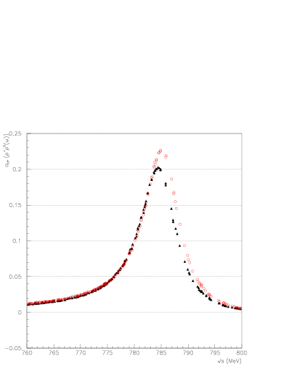
Figure 2: $CP$-violating asymmetry parameter, $a_{CP}(m)$, as a function of the ${\pi}^{+}{\pi}^{-}$ invariant mass in the vicinity of the $\omega$ mass region for the channel $B^{+}\rightarrow\rho^{0}(\omega)\rho^{+}\$ for two different form factor models.

References

- [1] I. Dunietz et al, Phys. Rev. D43 (1991) 2193.
- [2] Z.J. Ajaltouni et al, Eur.Phys.J. C 29, 215-233 (2003).
- [3] H. Quinn, ”Hadronic effects in two-body B decays”. Lectures at SLAC Summer Institute (1999).
- [4] A.J. Buras, Lect. Notes Phys. 558 (2000) 65, also in ‘Recent Developments in Quantum Field Theory’, Springer Verlag, edited by P. Breitenlohner, D. Maison and J. Wess (Springer-Verleg, Berlin, in press), hep-ph/9901409; R. Fleischer, Int. J. Mod. Phys. A12 (1997) 2459, Z. Phys. C62 (1994) 81, Z. Phys. C58 (1993) 483.
- [5] M. Bauer, B. Stech and M. Wirbel, Z. Phys. C34 (1987) 103; M. Wirbel, B. Stech and M. Bauer, Z. Phys. C29 (1985) 637.
-
[6]
C. Rimbault, PhD Thesis, DU1492 ”Etude de la violation directe de dans la
désintegration du méson en deux mésons vecteurs non charmés. Analyse
du canal dans le cadre de l’experience LHCb.” Université Blaise Pascal-Clermont
II (Février 2004)
O. Leitner, PhD Thesis, ”Direct violation in decays including mixing and covariant light-front dynamics”. - [7] M.Bander, D.Silverman, A.Soni, Phys.Rev.Let. 43 (1979) 242
- [8] B. Aubert et al (BaBar collaboration), ”Rates, Polarizations and asymmetries in Charmless Vector-Vector B Meson Decays”, Phys.Rev.Let. 91 (2003), 171802 and Phys.Rev. D69, 031102(R) (2004).
-
[9]
J. Zhang et al (Belle collaboration), ”Observation of ”
Phys.Rev.Let. 91 (2003), 221801 - [10] O. Leitner, X.-H. Guo, A.W.Thomas, Phys. Rev. D63 (2001) 056012.
- [11] O.Leitner, X.Guo, A.W.Thomas, Phys.Rev. D66 (2002), 096008