Color Superconductivity from Supersymmetry

Abstract

A supersymmetric composite model of color superconductivity is proposed. Quarks and diquarks are dynamically generated as composite fields by a newly introduced strong gauge dynamics. It is shown that the condensation of the scalar component of the diquark supermultiplet occurs when the chemical potential becomes larger than some critical value. We believe that the model well captures aspects of the diquark condensate behavior and helps our understanding of the diquark dynamics in real QCD. The results obtained here might be useful when we consider a theory composed of quarks and diquarks.

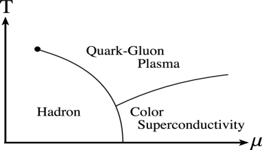
In the past few years, interesting properties of quark matter with nonzero temperature and baryon density such as the phase diagram in Fig. 1 have been extensively studied. In particular, color superconductivity CSC is one of the most promising possiblities to occur in such a system at low temperature because there exists an attractive interaction between quarks on the Fermi surface through the antisymmetric color $\bar{3}$ gluon exchange and it results in the quark-quark (not quark-antiquark) pairing, so-called diquark condensate. So far, a lot of people have tried to investigate this phenomena using different methods. At asymptotically high density, one can perform the weak coupling analysis of QCD and compute the superconducting gap son . On the other hand, at lower densities where the quark chemical potential $\mu$ is of order 500 MeV, since QCD itself is not tractable in this strong coupling regime and in addition there is a nortorious sign problem on the lattice Monte Carlo simulation with nonzero $\mu$, only some model studies (for instance, the Nambu-Jona-Lasinio model) which mimic crucial features of QCD such as chiral symmetry have been done so far NJL . According to these model studies, a phase transition between hadronic phase and color superconducting one is suggested to happen. Combining this with the result of the weak coupling analysis, we expect a similar phase structure is realized in dense QCD.

In the light of these current situations, the purpose of this paper is to propose some new way of understanding a system of dense quark matter based on supersymmetric (SUSY) QCD. In SUSY gauge theories, some exact nonperturbative results, which are powerful tools to study the strong coupling dynamics, have been already known review . It might be therefore interesting to investigate color superconductivity using SUSY gauge dynamics and consider whether we can obtain some insight into real QCD.

Figure 1: (Conjectured) phase diagram of hot and dense quark matter.

In HLM , symmetry breaking pattern was studied by using the exact results of SUSY QCD with nonzero chemical potetnial and was compared to that obtained from the analysis via nonsupersymmetric QCD schafer . One of the important observations is that the chemical potential can be incorpolated as the time component of a fictitious gauge field of the $U(1)_{B}$ baryon number symmetry at zero temperature, which leads to a tachyonic SUSY breaking scalar mass. However, gauge variant quantities such as the diquark degrees of freedom was not treated in their model. In order to see what happens to the system at large chemical potential, however, as has been already mentioned before, it is indispensable to include that degrees of freedom. Therefore in this paper we try to extend the work of HLM so as to involve gauge variant quantities at an intermediate energy range.

Along these line of thought, we propose a supersymmetric composite model of color superconductivity, in which quarks and diquarks appear as massless composites at low energy by a newly introduced strong coupling gauge dynamics, not by QCD dynamics. We find a certain parameter region where the scalar component of diquark supermultiplet condensation occurs when the chemical potetnial gets larger than some critical value. Although our model is not fully realistic in the sense that not diquarks themselves but the scalar component of the diquarks supermultiplet condense, nevertheless we believe that our model well captures some important aspects of the diquark condensate and helps our understanding for the color superconductivity in real QCD. The results obtained here may give an interesting insight on the phase structure at the intermediate region of the quark chemical potential.

Let us explain our model, which is based on a ${\cal N}=1$ SUSY $SO(N=N_{f}+4)$ gauge theory with $N_{f}$ vector representations IS . Its non-Abelian global symmetry $SU(N_{f})$ is extended to $SU(3)_{C}\times SU(N_{f})_{L}\times SU(N_{f})_{R}$ where $SU(3)_{C}$(usual color symmetry) gauge theory is assumed to be weakly gauged compared with $SO(N)$ gauge theory, ${\i.e.}\Lambda_{SO(N)}>\Lambda_{SU(3)_{C}}$ for the dynamical scales of each gauge group. Matter content is summarized below.

$$Q = (\>{\vbox{\vbox{\hrule height=0.6pt\hbox{\vrule width=0.6pt,height=5.0pt\kern 5.0pt\vrule width=0.6pt,height=5.0pt} \hrule height=0.6pt} }}\>\>,\>{\vbox{\vbox{\hrule height=0.6pt\hbox{\vrule width=0.6pt,height=5.0pt\kern 5.0pt\vrule width=0.6pt,height=5.0pt} \hrule height=0.6pt} }}\>\>,\>{\vbox{\vbox{\hrule height=0.6pt\hbox{\vrule width=0.6pt,height=5.0pt\kern 5.0pt\vrule width=0.6pt,height=5.0pt} \hrule height=0.6pt} }}\>\>,{\bf 1})_{1,1,1},$$ (1)

$$\bar{Q} = (\>{\vbox{\vbox{\hrule height=0.6pt\hbox{\vrule width=0.6pt,height=5.0pt\kern 5.0pt\vrule width=0.6pt,height=5.0pt} \hrule height=0.6pt} }}\>\>,\>\overline{{\vbox{\vbox{\hrule height=0.6pt\hbox{\vrule width=0.6pt,height=5.0pt\kern 5.0pt\vrule width=0.6pt,height=5.0pt} \hrule height=0.6pt} }}}\>\>,{\bf 1},\>\overline{{\vbox{\vbox{\hrule height=0.6pt\hbox{\vrule width=0.6pt,height=5.0pt\kern 5.0pt\vrule width=0.6pt,height=5.0pt} \hrule height=0.6pt} }}}\>\>)_{-1,1,1},$$ (2)

$$X = (\>{\vbox{\vbox{\hrule height=0.6pt\hbox{\vrule width=0.6pt,height=5.0pt\kern 5.0pt\vrule width=0.6pt,height=5.0pt} \hrule height=0.6pt} }}\>\>,{\bf 1},{\bf 1},{\bf 1})_{0,-6N_{f},3-N}$$ (3)

where the representations in the parenthesis are transformation properties under the group $SO(N)\times SU(3)_{C}\times SU(N_{f})_{L}\times SU(N_{f})_{R}$, where $N=6N_{f}+5$ in the present case. The numbers in the subscripts are charges for nonanomalous $U(1)$ global symmetries $U(1)_{B}\times U(1)_{A}\times U(1)_{R}$, which each $U(1)$ symmetries are linear combinations of the original anomalous $U(1)$ symmetries. $U(1)_{B}$ is a baryon number symmetry which plays an impotant role for considering the chemical potential effects. $U(1)_{A}$ is a non-R symmetry and $U(1)_{R}$ is an R-symmetry.

$SO(N)$ gauge theory under consideration is asymptotically free and known to be in a confining phase at the infrared (IR) IS . At the scale $\Lambda_{SO(N)}$, the theory becomes strongly coupled and $SO(N)$ gauge invariant composite fields appear as massless degrees of freedom in the low energy effective theory.

$$(Q^{2}) = (\>\overline{{\vbox{\vbox{\hrule height=0.6pt\hbox{\vrule width=0.6pt,height=5.0pt\kern 5.0pt\vrule width=0.6pt,height=5.0pt} \hrule height=0.6pt} }}}\>\>,\>{\vbox{\vbox{\hrule height=0.6pt\hbox{\vrule width=0.6pt,height=5.0pt\kern 5.0pt\vrule width=0.6pt,height=5.0pt} \hrule height=0.6pt\hbox{\vrule width=0.6pt,height=5.0pt\kern 5.0pt\vrule width=0.6pt,height=5.0pt} \hrule height=0.6pt} }}\>\>,{\bf 1})_{2,2,2},(\>{\vbox{\vbox{\hrule height=0.6pt\hbox{\vrule width=0.6pt,height=5.0pt\kern 5.0pt\vrule width=0.6pt,height=5.0pt\kern 5.0pt\vrule width=0.6pt,height=5.0pt} \hrule height=0.6pt} }}\>\>,\>{\vbox{\vbox{\hrule height=0.6pt\hbox{\vrule width=0.6pt,height=5.0pt\kern 5.0pt\vrule width=0.6pt,height=5.0pt\kern 5.0pt\vrule width=0.6pt,height=5.0pt} \hrule height=0.6pt} }}\>\>,{\bf 1})_{2,2,2},$$ (4)

$$(\bar{Q}^{2}) = (\>{\vbox{\vbox{\hrule height=0.6pt\hbox{\vrule width=0.6pt,height=5.0pt\kern 5.0pt\vrule width=0.6pt,height=5.0pt} \hrule height=0.6pt} }}\>\>,{\bf 1},\overline{\>{\vbox{\vbox{\hrule height=0.6pt\hbox{\vrule width=0.6pt,height=5.0pt\kern 5.0pt\vrule width=0.6pt,height=5.0pt} \hrule height=0.6pt\hbox{\vrule width=0.6pt,height=5.0pt\kern 5.0pt\vrule width=0.6pt,height=5.0pt} \hrule height=0.6pt} }}\>\>})_{-2,2,2},(\overline{\>{\vbox{\vbox{\hrule height=0.6pt\hbox{\vrule width=0.6pt,height=5.0pt\kern 5.0pt\vrule width=0.6pt,height=5.0pt\kern 5.0pt\vrule width=0.6pt,height=5.0pt} \hrule height=0.6pt} }}\>\>},{\bf 1},\overline{\>{\vbox{\vbox{\hrule height=0.6pt\hbox{\vrule width=0.6pt,height=5.0pt\kern 5.0pt\vrule width=0.6pt,height=5.0pt\kern 5.0pt\vrule width=0.6pt,height=5.0pt} \hrule height=0.6pt} }}\>\>})_{-2,2,2},$$ (5)

$$(X^{2}) = ({\bf 1},{\bf 1},{\bf 1})_{0,-12N_{f},6-2N},$$ (6)

$$(QX) = (\>{\vbox{\vbox{\hrule height=0.6pt\hbox{\vrule width=0.6pt,height=5.0pt\kern 5.0pt\vrule width=0.6pt,height=5.0pt} \hrule height=0.6pt} }}\>\>,\>{\vbox{\vbox{\hrule height=0.6pt\hbox{\vrule width=0.6pt,height=5.0pt\kern 5.0pt\vrule width=0.6pt,height=5.0pt} \hrule height=0.6pt} }}\>\>,{\bf 1})_{1,1-6N_{f},4-N},$$ (7)

$$(\bar{Q}X) = (\>\overline{{\vbox{\vbox{\hrule height=0.6pt\hbox{\vrule width=0.6pt,height=5.0pt\kern 5.0pt\vrule width=0.6pt,height=5.0pt} \hrule height=0.6pt} }}}\>\>,{\bf 1},\>\overline{{\vbox{\vbox{\hrule height=0.6pt\hbox{\vrule width=0.6pt,height=5.0pt\kern 5.0pt\vrule width=0.6pt,height=5.0pt} \hrule height=0.6pt} }}}\>\>)_{-1,1-6N_{f},4-N},$$ (8)

$$(Q\bar{Q}) = ({\bf 1},\>{\vbox{\vbox{\hrule height=0.6pt\hbox{\vrule width=0.6pt,height=5.0pt\kern 5.0pt\vrule width=0.6pt,height=5.0pt} \hrule height=0.6pt} }}\>\>,\>\overline{{\vbox{\vbox{\hrule height=0.6pt\hbox{\vrule width=0.6pt,height=5.0pt\kern 5.0pt\vrule width=0.6pt,height=5.0pt} \hrule height=0.6pt} }}}\>\>)_{0,2,2},({\bf 8},\>{\vbox{\vbox{\hrule height=0.6pt\hbox{\vrule width=0.6pt,height=5.0pt\kern 5.0pt\vrule width=0.6pt,height=5.0pt} \hrule height=0.6pt} }}\>\>,\>\overline{{\vbox{\vbox{\hrule height=0.6pt\hbox{\vrule width=0.6pt,height=5.0pt\kern 5.0pt\vrule width=0.6pt,height=5.0pt} \hrule height=0.6pt} }}}\>\>)_{0,2,2}$$ (9)

where the representations in the parenthesis are those under the group $SU(3)_{C}\times SU(N_{f})_{L}\times SU(N_{f})_{R}$. The numbers in the subscripts are charges for nonanomalous $U(1)$ symmetries $U(1)_{B}\times U(1)_{A}\times U(1)_{R}$. Note that $Q^{2}(\bar{Q}^{2})$ has symmetric (its conjugate) and anti-symmetric (its conjugate) representations under $SU(3)_{C}\times SU(N_{f})_{L}\times SU(N_{f})_{R}$ because $SO(N)$ indices are contracted symmetrically and the superfields are bosonic. The anti-symmetric ones correspond to “diquark” superfield responsible for the condensation when the chemical potential becomes larger than some critical value. $QX(\bar{Q}X)$ correspond to usual quarks (anti-quarks) superfields. Thus, quarks and diquarks coexist as massless composites in the low energy. As a nontrivial check that composite fields (4)–(9) are appropriate massless degrees of freedom, we can easily show that the ’t Hooft anomaly matching conditions for $[SU(N_{f})_{L,R}]^{3}$, $[SU(N_{f})_{L,R}]^{2}U(1)_{B,A,R}$, $U(1)_{B,A,R}$, $[U(1)_{B,A,R}]^{3}$, $[U(1)_{B,A}]^{2}U(1)_{R}$, $[U(1)_{A,R}]^{2}U(1)_{B}$, $[U(1)_{B,R}]^{2}U(1)_{A}$ at the origin of the moduli space are satisfied between elementary fields $Q,\bar{Q},X$ and all composite fields (4)–(9).

The low energy effective superpotential is generated by the gaugino condensation in the unbroken gauge group $SO(N)\to SO(4)\simeq SU(2)_{L}\times SU(2)_{R}$;

$$W_{{\rm eff}}=2(\epsilon_{L}+\epsilon_{R})\left(\frac{\Lambda_{SO(N)}^{6N_{f}+4}}{[{\rm det}(Q\bar{Q})]X}\right)$$ (10)

where $\epsilon_{L,R}=\pm 1$ are phase factors reflecting the number of SUSY vacua suggested from Witten index Witten .

Since our interest is whether the condensation of the scalar component of the diquark supermultiplet occurs or not as the chemical potential changes, we need to estimate the soft scalar mass squareds for composite fields, whose sign indicate whether composite fields develop vacuum expectation values (VEVs) or not. In softly broken SUSY gauge theory, it is well known that soft scalar masses in the IR region can be derived from those in the ultraviolet (UV) region by the procedure in Ref. AR . The effective Kähler potential for composite fields is fixed by symmetries and the renormalization group (RG) invariance,

$$K_{{\rm eff}} = c_{(Q^{2})}\frac{{\cal Z}_{(Q^{2})}}{I}(Q^{2})^{\dagger}e^{2V_{B}}(Q^{2})$$ (11)

$$+ c_{(\bar{Q}^{2})}\frac{{\cal Z}_{(\bar{Q}^{2})}}{I}(\bar{Q}^{2})^{\dagger}e^{-2V_{B}}(\bar{Q}^{2})$$

$$+ c_{(X^{2})}\frac{{\cal Z}_{(X^{2})}}{I}(X^{2})^{\dagger}(X^{2})$$

$$+ c_{(QX)}\frac{{\cal Z}_{(QX)}}{I}(QX)^{\dagger}e^{V_{B}}(QX)$$

$$+ c_{(\bar{Q}X)}\frac{{\cal Z}_{(\bar{Q}X)}}{I}(\bar{Q}X)^{\dagger}e^{-V_{B}}(\bar{Q}X)$$

$$+ c_{(Q\bar{Q})}\frac{{\cal Z}_{(Q\bar{Q})}}{I}(Q\bar{Q})^{\dagger}(Q\bar{Q}),$$

where overall coefficients $c$’s are of order ${\cal O}(1)$ unknown constants. The exponential factors for QCD are suppressed. $V_{B}$ is a background vector superfield $U(1)_{B}$ with a VEV $\langle V_{B}\rangle=\bar{\theta}\sigma^{\mu}\theta\langle A_{\mu}\rangle,\quad\langle A_{\mu}\rangle=(\mu/g_{B},0,0,0)$. $g_{B}$ is a gauge coupling constant and $\mu$ is a chemical potential, which breaks SUSY explicitly. Therefore, we assume $\mu\ll\Lambda_{SO(N)}$ so that we can make use of exact results of the SUSY gauge theory. This VEV of the background vector field provides additional tachyonic soft SUSY breaking scalar mass squareds as discussed in HLM . Wave function renomalization constants $Z_{i}$ are promoted to a superfield ${\cal Z}_{i}$

$${\cal Z}_{i}=Z_{i}\left[1-\theta^{2}\bar{\theta}^{2}m_{{\rm soft}}^{2}\right]$$ (12)

where $m_{{\rm soft}}$ is a soft SUSY breaking scalar mass in the UV and taken to be universal. The quantity $I$ is a spurious $U(1)$ symmetry and the RG invariant superfield,

$$I=\Lambda_{h}^{\dagger}{\cal Z}^{2T/b_{0}}\Lambda_{h}$$ (13)

where $T$ is the total Dynkin index of the matter fields, $b_{0}$ is the 1-loop beta function coefficient and $\Lambda_{h}=\mu_{UV}{\rm exp}[-8\pi^{2}S(\mu_{UV})/b_{0}],S(\mu_{UV})=\frac{1}{g^{2}}\left(1+\theta^{2}\frac{m_{\lambda}}{2}\right)(m_{\lambda}:{\rm gaugino~{}mass})$. Note that a spurious $U(1)$ transformations are given by

$$Q_{r}\to e^{A}Q_{r},{\cal Z}_{r}\to e^{A+A^{\dagger}}{\cal Z}_{r},$$ (14)

$$S(\mu_{{\rm UV}})\to S(\mu_{{\rm UV}})-\frac{T}{4\pi^{2}}A$$ (15)

where $A$ is a chiral superfield.

Now, the soft SUSY breaking scalar masses for composites with the canonical kinetic term are obtained by taking $\theta^{2}\bar{\theta}^{2}$ terms in Eq. (11) footnote1 ,

$$\tilde{m}^{2}_{(Q^{2})}=\tilde{m}^{2}_{(\bar{Q}^{2})} = \frac{6N_{f}+7}{2(3N_{f}+2)}m_{{\rm soft}}^{2}-\mu^{2},$$ (16)

$$\tilde{m}^{2}_{(X^{2})}=\tilde{m}^{2}_{(Q\bar{Q})} = \frac{6N_{f}+7}{2(3N_{f}+2)}m^{2}_{{\rm soft}}>0,$$ (17)

$$\tilde{m}^{2}_{(QX)}=\tilde{m}^{2}_{(\bar{Q}X)} = \frac{6N_{f}+7}{2(3N_{f}+2)}m_{{\rm soft}}^{2}-\frac{1}{4}\mu^{2}.$$ (18)

For the case $\epsilon_{L}=-\epsilon_{R}$ with vanishing superpotetnial in (10), the scalar potetntial consists of only the soft scalar masses (16)–(18). We then immediately find from (16) that $\tilde{m}^{2}_{(Q^{2})}=\tilde{m}^{2}_{(\bar{Q}^{2})}<0$ for $\mu>\mu_{*}(\equiv\sqrt{\frac{6N_{f}+7}{2(3N_{f}+2)}}m_{{\rm soft}}>m_{{\rm soft}})$. This means that $\langle Q^{2}\rangle,\langle\bar{Q}^{2}\rangle\neq 0$ in that range of the chemical potential footnote2 .

Furthermore, if we take into account the most attractive channel hypothesis MAC , anti-symmetric part of $Q^{2}(\>\overline{{\vbox{\vbox{\hrule height=0.6pt\hbox{\vrule width=0.6pt,height=5.0pt\kern 5.0pt\vrule width=0.6pt,height=5.0pt} \hrule height=0.6pt} }}}\>\>,\>{\vbox{\vbox{\hrule height=0.6pt\hbox{\vrule width=0.6pt,height=5.0pt\kern 5.0pt\vrule width=0.6pt,height=5.0pt} \hrule height=0.6pt\hbox{\vrule width=0.6pt,height=5.0pt\kern 5.0pt\vrule width=0.6pt,height=5.0pt} \hrule height=0.6pt} }}\>\>,{\bf 1})_{2,2,2},\bar{Q}^{2}(\>{\vbox{\vbox{\hrule height=0.6pt\hbox{\vrule width=0.6pt,height=5.0pt\kern 5.0pt\vrule width=0.6pt,height=5.0pt} \hrule height=0.6pt} }}\>\>,{\bf 1},\overline{\>{\vbox{\vbox{\hrule height=0.6pt\hbox{\vrule width=0.6pt,height=5.0pt\kern 5.0pt\vrule width=0.6pt,height=5.0pt} \hrule height=0.6pt\hbox{\vrule width=0.6pt,height=5.0pt\kern 5.0pt\vrule width=0.6pt,height=5.0pt} \hrule height=0.6pt} }}\>\>})_{-2,2,2}$ are likely to have VEVs since the force acting on $Q^{2}$ or $\bar{Q}^{2}$ by one $SO(N)$ gauge boson exchange is attractive. On the other hand, the force is replusive in the symmetric case. This is our main result that we wish to show.

We also note that $\mu_{*}>m_{{\rm soft}}$ implies $\mu>m_{{\rm soft}}$ for the condensation of the scalar component of the diquark supermultiplet to occur. This leads to UV unstable theory since the soft SUSY breaking scalar mass squared in the UV becomes negative in the presence of the chemical potential, $\tilde{m}^{2}_{Q}=m_{{\rm soft}}^{2}-\mu^{2}<0$. We therefore add SUSY mass terms

$$W=m_{ij}Q_{i}\bar{Q}_{j},\quad m_{ij}=m\delta_{ij}$$ (19)

where the mass is taken to be flavor diagonal to preserve the most global symmetry. For the UV theory to be stable, $\sqrt{m^{2}+m_{{\rm soft}}^{2}}>\mu$ is required. The SUSY mass term (19) can be rewritten in the IR as the linear term of composite,

$$W=m(Q\bar{Q}),$$ (20)

which breaks SUSY spontaneously. We also have to impose the condition $m\ll\Lambda_{SO(N)}$ to use the exact results of SUSY gauge theory reliably.

Combining these facts, we can obtain the diquark supermultiplet the scalar component of the diquark supermultiplet condenses at some critical value of chemical potenial $\mu_{*}$. We cannot determine exactly where the scalar component of the diquark supermultiplet stabilize, but in a region where the field VEV is much larger than $\Lambda_{SO(N)}$, elementary fields are appropriate variables, we know that the potential is stabilized by SUSY mass terms. This implies that the VEVs of the scalar component of the diquark supermultiplet should be stabilized at certain value.

One may find from (18) that composite squarks develop VEVs $\langle QX\rangle,\langle\bar{Q}X\rangle\neq 0$ for $\mu>2\mu_{*}$ if $2\mu_{*}<\sqrt{m^{2}+m_{{\rm soft}}^{2}}$. However, the scalar component of the diquark supermultiplet condenses as far as the chemical potential is larger than the critical chemical potential value $\mu_{*}$. In order to analyze the theory in such a case, we have to expand our theory around the VEV of the scalar component of the diquark supermultiplet condensation. Therefore, the above description of the squark condensation is left untouched at the present stage.

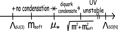
Figure 2: Relation among various scales are displayed. Horizontal axis means the energy scale. The possible range of the chemical potential is below $\sqrt{m^{2}+m^{2}_{{\rm soft}}}$. There is no condensation when the chemical potential is between QCD scale $\Lambda_{{\rm SU(3)}}$ and the critical chemical potential $\mu_{*}$. The condensation of the scalar component of the diquark supermultiplet occurs when the chemical potential is between $\mu_{*}$ and $\sqrt{m^{2}+m^{2}_{{\rm soft}}}$. UV theory becomes unstable if the chemical potetntial is beyond the scale $\sqrt{m^{2}+m^{2}_{{\rm soft}}}$.

The above argument for the behavior of the scalar component of the diquark supermultiplet or squark supermultiplet condensation is valid for the vanishing superpotential with $\epsilon_{L}=-\epsilon_{R}$ in (10). For the case with $\epsilon_{L}=\epsilon_{R}$, on the other hand, it is found that the scalar potenial is very complicated,

$$V = \left(\frac{\partial^{2}K_{{\rm eff}}}{\partial\Phi_{i}\partial\Phi^{*}_{j}}\right)^{-1}\left(\frac{\partial W_{{\rm eff}}}{\partial\Phi_{i}}\right)\left(\frac{\partial W^{*}_{{\rm eff}}}{\partial\Phi^{*}_{j}}\right)\Lambda^{2}_{SO(N)}$$ (21)

$$+ \frac{1}{\Lambda^{2}_{SO(N)}}\left[\tilde{m}^{2}_{(Q^{2})}|(Q^{2})|^{2}+\tilde{m}^{2}_{(\bar{Q}^{2})}|(\bar{Q}^{2})|^{2}\right.$$

$$+ \left.\tilde{m}^{2}_{(X^{2})}|(X^{2})|^{2}+\tilde{m}^{2}_{(QX)}|(QX)|^{2}\right.$$

$$+ \left.\tilde{m}^{2}_{(\bar{Q}X)}|(\bar{Q}X)|^{2}+\tilde{m}^{2}_{(Q\bar{Q})}|(Q\bar{Q})|^{2}\right]$$

where $\Phi_{i}$ denote the scalar component of composite superfields, $K_{{\rm eff}}$ is given by (11) and $W_{{\rm eff}}$ is the sum of the superpotential (10) rewritten in terms of composites and (20). Therefore, we give here a qualitative discussion on the scalar potential behavior instead of performing an explicit minimization of the scalar potential. Note that F-term contributions to the scalar potential in the first line of (21) have a runaway behavior, which make the fields VEV away from the origin. For $\mu=0$, all SUSY breaking scalar mass squareds are positive, which set the fields VEV at the origin. Therefore all composites are expected to develop nonvanishing VEVs by balancing terms between the runaway potential and the SUSY breaking scalar mass terms. Even if we take into account that the scalar diquark mass squareds become negative for $\mu>\mu_{*}$, qualitative features of phase transition remains unchanged. In any case, the case of nonzero superpotential with $\epsilon_{L}=\epsilon_{R}$ in (10) is irrelevant to the phase of color superconductivity of our interest. Even if we compare the vacuum energy in both cases, the case with vanishing superpotential seems to be energetically favored.

In summary, motivated by the work of HLM , we have tried to construct a toy model where gauge noninvariant operators are taken into account in SUSY gauge theories. We have proposed a SUSY composite model of color superconductivity, which is based on an $SO(N)$ gauge theory with $(N-4)$ vector representations IS . Our model is in a confining phase for $SO(N)$ gauge dymanics at low energies, in which quarks and diquarks are generated dynamically as composite fields satisfying anomaly matching conditions. We have shown that the scalar component of the diquark supermultiplet condensate occurs when the chemical potential becomes larger than some critical value $\mu_{*}=\sqrt{\frac{6N_{f}+7}{2(3N_{f}+2)}}m_{{\rm soft}}$. Our model is valid in the parameter region $\Lambda_{{\rm SU(3)}}<\mu<\sqrt{m^{2}+m^{2}_{{\rm soft}}}$, where the upper bound is required for the theory to be stable in the UV and the lower bound implies that we consider the theory where quarks are deconfined. Although the model is not fully realistic in that the scalar component of diquark supermultiplet (not diquarks themselves) condense, we believe that it well captures some important aspects of the diquark condensation behavior and helps our understanding for the color superconductivity in real QCD. If there is a certain intermediate region of the chemical potential where quarks are deconfined but not superconducting yet, owing to the strong quark-quark correlation, the system may be well described by a compositon of quarks and diquarks. Then the analysis performed in this paper will help us with comprehending the behavior of such a system.

As future directions, it is interesting to extend our analysis to other flavor cases with various phases other than the confining phase. In particular, it might be possible to obtain better and more realistic understanding for the diquark condensation behavior by exploiting Seiberg dual magnetic description Seiberg . In order to fully understand the phase structure of QCD, it is necessary to take into account the finite temperature effects. It is therefore indispensable to consider our model extended to five dimensional spacetime compactified on $S^{1}$, and then to study the scalar component of the diquark supermultiplet condensation behavior on the temperature-chemical potential plane as shown in Fig 1.