Particle abundance in a thermal plasma:
quantum kinetics vs. Boltzmann equation

Abstract

We study the abundance of a particle species in a thermalized plasma by introducing a quantum kinetic description based on the non-equilibrium effective action. A stochastic interpretation of quantum kinetics in terms of a Langevin equation emerges naturally. We consider a particle species that is stable in the vacuum and interacts with heavier particles that constitute a thermal bath in equilibrium. Asymptotic theory suggests a definition of a fully renormalized single particle distribution function. Its real time dynamics is completely determined by the non-equilibrium effective action which furnishes a Dyson-like resummation of the perturbative expansion. The distribution function reaches thermal equilibrium on a time scale $\sim 1/2\,\Gamma_{k}(T)$ with $\Gamma_{k}(T)$ being the quasiparticle relaxation rate. The equilibrium distribution function depends on the full spectral density as a consequence the fluctuation-dissipation relation. Such dependence leads to off-shell contributions to the particle abundance. A specific model of a bosonic field $\Phi$ in interaction with two heavier bosonic fields $\chi_{1,2}$ is studied. The decay of the heaviest particle and its recombination lead to a width of the spectral function for the particle $\Phi$ and to off-shell corrections to the abundance. We find substantial departures from the Bose-Einstein result both in the high temperature and the low temperature but high momentum region. In the latter the abundance is exponentially suppressed but larger than the Bose-Einstein result. We obtain the Boltzmann equation in renormalized perturbation theory and highlight the origin of the differences. Cosmological consequences are discussed: we argue that the corrections to the abundance of cold dark matter candidates are observationally negligible and that recombination erases any possible spectral distortions of the CMB. However we expect that the enhancement at high temperature may be important for baryogenesis.

I Introduction

Phenomena out of equilibrium played a fundamental role in the early Universe: during phase transitions, baryogenesis, nucleosynthesis, recombination, particle production, annihilation and freeze out of relic particles, some of which could be dark matter candidateskolbturner ; bernstein ; dodelson . Of the many different non-equilibrium processes, particle production, annihilation and freeze-out and baryogenesiskolbturner ; buchmuller are non-equilibrium kinetic processes which are mainly studied via the Boltzmann equationkolbturner ; bernstein ; dodelson .

The Boltzmann kinetic equation is also the main approach to study equilibration, thermalization and abundance of a species in a plasma. A thorough formulation of semiclassical kinetic theory in an expanding Friedmann-Robertson-Walker cosmology is given in ref.bernstein .

However the Boltzmann equation is a classical equation for the distribution function with an inhomogeneity determined by collision terms which are computed with the S-matrix formulation of quantum field theory. The collision term in the Boltzmann equation is obtained from the transition probability per unit time extracted from the asymptotic long time limit of the transition matrix element. This is tantamount to implementing Fermi’s golden rule. Potential quantum interference and memory effects are completely ignored in this approach. Furthermore a single particle distribution function, the main ingredient in the Boltzmann equation, is usually defined via some coarse graining procedure. All of these shortcomings of the usual semiclassical Boltzmann equations when extrapolated to the realm of temperatures and density in the Early Universe, suggest that in order to provide a reliable understanding of such delicate processes such as baryo and leptogenesis a full quantum field theory treatment of kinetics may be requiredbuchmuller .

One of the basic predictions of the Boltzmann equation is that the local thermodynamic equilibrium solution for the abundance of a particle species is determined by the Bose-Einstein or Fermi-Dirac distribution functions, hence exponentially suppressed at low temperatures (in absence of a chemical potential).

This basic prediction has recently been challenged in a series of articlesyoshimura wherein a surprising result is obtained: the abundance of heavy particles with masses much larger than the temperature is not exponentially suppressed as the Boltzmann equation predicts but the suppression is a power law. Such result, if correct, can have important consequences for the relic abundance of cold dark matter candidates.

This result, however, has been criticized and scrutinized in detail by several authorssrednicki ; jia ; pietroni who concluded that it is a consequence of the definition of the particle number introduced in ref.yoshimura . The definition of the total number of particles proposed in yoshimura is based on the non-interacting Hamiltonian for the heavy particle divided by its mass plus counterterms, which purportedly account for renormalization effects. The results of referencessrednicki ; jia ; pietroni point out the inherent ambiguity in separating the contribution to the energy density from the particle and that of the bath and the interaction. The ambiguity in the separation of the different contributions to the energy has been studied thoroughly in these references in particular exactly solvable modelssrednicki , effective field theoryjia or a consistent treatment of renormalization effectspietroni .

Understanding the limitations of and corrections to the Boltzmann kinetic description and potential departures from the predicted abundances is important for a deeper assessment of possible mechanisms of baryogenesis as well as for the relic abundance of cold dark matter candidates. In the case of baryogenesis, the applicability and reliability of Boltzmann kinetics in the conditions of temperature and density that prevailed in the early Universe warrants a critical reassessmentbuchmuller . Refinements of the usual Boltzmann equation have been proposed in the literaturejakovac .

While the work in refs.srednicki ; jia ; pietroni has clarified the shortcomings of the definition of the total particle number proposed inyoshimura explaining the origin of the power law suppression as a consequence of the ambiguity in this definition, what is missing from this discussion is a suitable definition of a distribution function and its real time evolution. The Boltzmann equation is a local differential equation that determines the dynamics of the single particle distribution function. Therefore in order to clearly assess potential corrections to the equilibrium solutions of the familiar Boltzmann equation a suitable distribution function and its dynamical evolution must be understood.

The definition of the distribution function both in non-relativistic many body theorybaym as well as in relativistic quantum field theorymalfliet ; calzetta is typically based on a Wigner transform of a two point correlation function, which is not manifestly positive semidefinite. Usual derivations of the Boltzmann kinetic equation invoke gradient expansions or quasiparticle (on-shell) approximations which lead to Markovian dynamics. Alternative derivations of the kinetic equationsboyaboltz which explicitly implement real time perturbation theory often invoke a long time limit and Fermi’s Golden rule which enforces energy conservation in the kinetic equation. This is also the case in the dynamical renormalization group approach to quantum kinetics advocated in ref.drg although this latter method allows one to systematically include off-shell corrections. Whichever method of derivation of the kinetic equation is used, the first step is to define a single particle distribution function.

Any definition of the distribution function of particles that decay in the vacuum (resonances) is fraught with ambiguities because the spectral representation of such particles is not a sharp delta function but typically a Breit-Wigner distribution. Since these particles decay even in vacuum and do not exist as asymptotic states any definition of an operator that “counts” these particles will unavoidably be ambiguous.

In this work, we circumvent this ambiguity by focusing on the study of the quantum kinetics and equilibration dynamics of the distribution functions of particles that are stable at zero temperature associated with a field $\Phi$. Stable physical particles are asymptotic states which can be measured and a distribution function for the single particle physical states can be introduced according to the basic assumptions of asymptotic theory. While our ultimate goal is to find a quantum kinetic description for phenomena in the early Universe, in this article we focus on a study in Minkowski space-time as a first step towards that goal.

Goals and methods:

In this article we provide a framework for non-equilibrium quantum kinetics beyond the usual Boltzmann equation. This non-equilibrium formulation includes off-shell and non-Markovian (memory) processes which are not accounted for in the semiclassical Boltzmann equation and result in modifications of the equilibrium abundances. We focus on the case of a scalar field $\Phi$ coupled to other heavier fields for a wide variety of relevant interacting quantum field theories. Here we consider that the heavier fields constitute a thermal bath in equilibrium. In order to study the thermalization of the $\Phi$ particle as well as the time evolution of its distribution function we consider the case in which the field $\Phi$ is coupled to the thermal bath at some initial time $t_{i}$. We then obtain the non-equilibrium effective action for the field $\Phi$ by integrating out the degrees of freedom of the thermal bath to lowest order in the coupling of the field $\Phi$ to the heavy sector but in principle to all orders in the couplings of the heavy fields amongst themselves.

At zero temperature the $\Phi$-particles are stable because they are the lightest, therefore they are manifest as asymptotic states. Hence according to asymptotic theory we introduce a definition of an interpolating number operator that counts these particles, for example as those measured by a detector in a collision experiment in the vacuum. At finite temperature the distribution function is the expectation value of this interpolating operator in the statistical ensemble. The real time evolution of this distribution function is completely determined by the non-equilibrium effective action and its asymptotic long time limit determines the abundance of the physical particles $\Phi$ in the thermal plasma. The non-equilibrium approach introduced here, borrows from the seminal work on quantum Brownian motionschwinger ; feyver ; leggett ; grabert which is adapted to quantum field theory.

After the discussion of the general case, we introduce a specific model in which the scalar field $\Phi$ associated with the stable particle couples to two heavier bosonic fields which constitute the thermal bath. At lowest order in the coupling we find that the $\Phi$ particle despite being the lightest, acquires a width in the medium as a consequence of the two body decay of the heavier particle and its recombination in the plasma. These processes result in a broadening of its spectral function and corrections to its equilibrium abundance.

Brief summary of results:

• We obtain the non-equilibrium effective action for a field $\Phi$ coupled to other heavier fields by integrating out the latter to lowest order in their coupling to the field $\Phi$ but in principle to all orders in the couplings amongst themselves. The heavy fields are taken to be in thermal equilibrium and therefore provide a thermal “bath” for the $\Phi$ field. The resulting non-equilibrium effective action can be interpreted as a generating functional of a stochastic field theory in which the (integrated out) heavy fields introduce a Gaussian but colored noise and a non-Markovian self-energy (dissipative) kernel.

• We introduce a definition of the single particle distribution function in the general case of a particle that is stable in the vacuum. Stable physical particles are asymptotic states which can be measured by a detector. In accordance with the results of asymptotic theory, we introduce a fully renormalized interpolating number operator whose expectation value in the non-equilibrium state (density matrix) is identified with the single particle distribution function. The time evolution of this distribution function is determined by the non-equilibrium effective action and is completely specified by the solution of a stochastic Langevin equation with a memory kernel and a Gaussian stochastic noise. The properties of the memory kernel are related to the spectrum of the noise by a generalized fluctuation dissipation relation. We argue that the time evolution of the distribution function is a result of a Dyson resummation of the perturbative expansion provided by the non-equilibrium effective action. The single particle distribution function becomes insensitive to the initial conditions at time scales longer than the “quasiparticle” relaxation time and its asymptotic long time limit describes a thermalized state.

• A specific example is studied in detail. This is a model of Bosonic scalar fields with a coupling $g\,\Phi\,\chi_{1}\,\chi_{2}$ with the masses of the “bath” fields $\chi_{1,2}$ obeying the hierarchy $M_{1}>M_{2}>>M_{\Phi}$. In this case the particles associated with the field $\Phi$ are stable in the vacuum. However, at finite temperature the particle $\Phi$ acquires a width from the two-body decay and recombination process $\chi_{1}\leftrightarrow\Phi+\chi_{2}$. We study the approach to thermal equilibrium of the single $\Phi$ particle distribution function whose asymptotic long time limit yields their equilibrium abundance in the bath. We find that the equilibrium abundance is always larger than that predicted by the Bose-Einstein distribution. The enhancement is more significant at high temperatures, as well as at low temperatures but large momenta. The departure from the Bose-Einstein result is a distinct consequence of off-shell support of the spectral function of the $\Phi$ field in the plasma.

• We derive the usual quantum kinetic Boltzmann equation in renormalized perturbation theory up to the same order in the coupling to the bath as the non-equilibrium effective action. This derivation highlights the neglect of memory and correlations in the usual Boltzmann equation. We contrast its prediction for the equilibrium abundance, the usual Bose-Einstein distribution, to that from the full quantum kinetic equation with memory and off-shell contributions. This direct comparison leads to the conclusion that memory and off-shell phenomena result in substantial corrections to the equilibrium abundances that are not captured by the Boltzmann equation.

• We conclude that potential corrections to the abundance of cold dark matter candidates as well as distortions of the cosmic microwave background post recombination are negligible observationally, but substantial corrections in a high temperature plasma may be important for baryogenesis.

The article is organized as follows: in section (II) we introduce the general form of the interacting quantum field theories considered and develop the formulation in terms of the non-equilibrium effective action. The effective action is obtained to lowest order in the coupling of the field $\Phi$ to the heavier fields (the bath) and in principle to all orders in the coupling of the bath fields amongst themselves. We show that a stochastic formulation in terms of a Langevin equation emerges naturally. In section (III) we introduce the definition of the fully renormalized interpolating number operator and the single particle distribution function based on asymptotic theory. The time evolution of this distribution function is completely determined by the solution of the stochastic Langevin equation.

In section (IV) we study a specific model in which the $\Phi$ field is coupled to two heavy scalar fields with a coupling $g\,\Phi\,\chi_{1}\,\chi_{2}$. This interacting quantum field theory provides an excellent testing ground and highlights the main conceptual results. We study the dynamics of the distribution function for the $\Phi$ particle up to one loop order. The asymptotic distribution function is studied for a wide range of parameters allowing to extract fairly general conclusions whose validity goes beyond this specific model. In particular we analyze in detail how off-shell effects result in large corrections to the usual Bose-Einstein equilibrium abundance. In section (V) we obtain the usual Boltzmann quantum kinetic equation and highlight the main assumptions implicit in its derivation. We contrast the predictions for the asymptotic abundance between the non-equilibrium kinetic formulation and that of the usual quantum kinetic Boltzmann equation, highlighting that memory and off-shell effects are responsible for the differences in the predictions. Our conclusions and a discussion on the cosmological consequences are presented in section (VI). An appendix is devoted to the explicit calculation of the self-energy in the specific example studied.

II General formulation: the non-equilibrium effective action

We focus on the description of the dynamics of the relaxation of the occupation number of a scalar field $\Phi$ which is in interaction with other fields either fermionic or bosonic, collectively written as $\chi_{i}$, with a Lagrangian density of the form

$${\cal L}[\Phi(x),\chi(x)]={\cal L}_{0,\Phi}[\Phi(x)]+{\cal L}_{\chi_{i}}[\chi_{i}(x)]+g\Phi{\cal O}[\chi_{i}(x)]$$ (1)

where ${\cal O}[\chi_{i}]$ stands for an operator non-linear in the fields $\chi_{i}$ and ${\mathcal{L}}_{0,\Phi}$ is the free field Lagrangian density for the field $\Phi$ but ${\cal L}_{\chi_{i}}[\chi_{i}(x)]$ is the full Lagrangian for the fields $\chi$ including interactions amongst themselves. This general form describes several relevant cases:

• Interacting scalars, for example the linear sigma model in the broken symmetry phase. The interaction between the massive scalar and the Goldstone bosons is of the form $\sigma\pi^{2}$. In this article we focus on the case of a trilinear interaction of the form $\Phi\sum_{ij}g_{ij}\chi_{i}\chi_{j}$ where the fields $\chi_{1,2}$ have masses larger than that of the $\Phi$ field.

• A Yukawa theory with $\chi$ being fermionic fields and $\Phi$ a scalar field, with interaction $\Phi\bar{\Psi}\Psi$. This could be generalized to a chiral model.

• A gauge theory in which $\Phi$ is the gauge field and $\chi$ is either a complex scalar or fermion fields, the interaction being of the form $A^{\mu}J_{\mu}$ with $J_{\mu}$ being a bilinear of the fields. In particular this approach has been recently implemented to study photon production from a quark gluon plasma in local thermal equilibriumboyphoton . This case is particularly relevant for assessing potential distortions in the spectrum of the cosmic microwave background.

• Another possible realization of this situation could be the case in which $\Phi$ is a neutrino field in interaction with leptons and (or) quarks which constitute a thermal or dense plasma.

• The case of a self-interacting scalar field in which one mode say with wave vector $k$ is singled out as the “system” and the other modes are treated as a “bath”.

In all of these cases the fields $\chi_{i}$ are treated as a bath in equilibrium assuming that the bath fields are sufficiently strongly coupled so as to guarantee their thermal equilibration. These fields will be “integrated out” yielding a reduced density matrix for the field $\Phi$ in terms of an effective real-time functional, known as the influence functionalfeyver in the theory of quantum brownian motion. The reduced density matrix can be represented by a path integral in terms of the non-equilibrium effective action that includes the influence functional. This method has been used extensively to study quantum brownian motionfeyver ; leggett ; grabert and for preliminary studies of quantum kinetics in the simpler case of a particle coupled linearly to a bath of harmonic oscillatorsboyalamo ; yoshimura .

The models can be generalized further by considering that the interaction between $\Phi$ and $\chi$ is also polynomial in $\Phi$. However, in this article we will consider the simpler case described by (1) since it describes a broad range of physically relevant cases, and as will be discussed below this case already reveals a wealth of novel phenomena. As we will discuss in detail below most of the relevant phenomena can be highlighted within this wide variety of models and most of the results will be seen to be fairly general.

The relaxation of the distribution function is an initial value problem, therefore we propose the initial density matrix at a time $t_{i}$ to be of the form

$$\hat{\rho}(t_{i})=\hat{\rho}_{\Phi,i}\otimes\hat{\rho}_{\chi_{i},i}$$ (2)

The initial density matrix of the $\chi_{i}$ fields will be taken to describe state in thermal equilibrium at a temperature $T=1/\beta$, namely

$$\hat{\rho}_{\chi}=e^{-\beta\,H_{\chi}}$$ (3)

where $H_{\chi_{i}}(\chi_{i})$ is the Hamiltonian for the fields $\chi_{i}$. We will now refer collectively to the set of fields $\chi_{i}$ simply as $\chi$ to avoid cluttering of indices.

In the field basis the matrix elements of $\hat{\rho}_{\Phi,i}$ are given by

$$\langle\Phi|\hat{\rho}_{\Phi,i}|\Phi^{\prime}\rangle=\rho_{\Phi,i}(\Phi;\Phi^{\prime})$$ (4)

The density matrix for $\Phi$ will represent an initial out of equilibrium state.

The physical situation described by this initial state is that of a field (or fields) in thermal equilibrium at a temperature $T=1/\beta$, namely a heat bath, which is put in contact with another system, here represented by the field $\Phi$. Once the system and bath are put in contact their mutual interaction will eventually lead to a state of thermal equilibrium. The goal is to study the relaxation of the field $\Phi$ towards equilibrium with the “bath”. The initial density matrix of the field $\Phi$ will describe a state with few quanta (or the vacuum) initially.

The real time evolution of this initial uncorrelated state will introduce transient evolution, however the long time behavior will be insensitive to this initial transient. Furthermore, we point out that it is important to study the initial transient stage for the following reason. As a particle $\Phi$ propagates in the medium it will be screened or dressed by the excitations in the medium and it will propagate as a “quasiparticle”. Its distribution function will be shown to become insensitive to the initial conditions on time scales larger than the “quasiparticle” relaxation time.

The strategy is to integrate out the $\chi$ fields therefore obtaining the reduced time dependent density matrix for the field $\Phi$, and the non-equilibrium influence functional for this field. Once we obtain the reduced density matrix for the field $\Phi$ we can compute expectation values or correlation functions of this field. We will focus on studying the time evolution of the distribution function, or particle number to be defined below.

The time evolution of the initial density matrix is given by

$$\hat{\rho}(t_{f})=e^{-iH(t_{f}-t_{i})}\hat{\rho}(t_{i})e^{iH(t_{f}-t_{i})}$$ (5)

Where the total Hamiltonian $H$ is given by

$$H=H_{\Phi}(\Phi)+H_{\chi}(\chi)+H_{I}(\Phi,\chi)$$ (6)

The calculation of correlation functions is facilitated by introducing currents coupled to the different fields. Furthermore since each time evolution operator in eqn. (5) will be represented as a path integral, we introduce different sources for forward and backward time evolution operators, referred to as $J^{+},J^{-}$ respectively. The forward and backward time evolution operators in presence of sources are $U(t_{f},t_{i};J^{+})$, $U^{-1}(t_{f},t_{i},J^{-})$ respectively.

We will only study correlation functions of the $\Phi$ field, therefore we carry out the trace over the $\chi$ degrees of freedom. Since the currents $J^{\pm}$ allow us to obtain the correlation functions for any arbitrary time by simple variational derivatives with respect to these sources, we can take $t_{f}\rightarrow\infty$ without loss of generality.

The non-equilibrium generating functional is given by

$${\cal Z}[j^{+},j^{-}]=\mathrm{Tr}U(\infty,t_{i};J^{+})\hat{\rho}(t_{i})U^{-1}(\infty,t_{i},J^{-})$$ (7)

Where $J^{\pm}$ stand collectively for all the sources coupled to different fields. Functional derivatives with respect to the sources $J^{+}$ generate the time ordered correlation functions, those with respect to $J^{-}$ generate the anti-time ordered correlation functions and mixed functional derivatives with respect to $J^{+},J^{-}$ generate mixed correlation functions. Each one of the time evolution operators in the generating functional (7) can be written in terms of a path integral: the time evolution operator $U(\infty,t_{i};J^{+})$ involves a path integral forward in time from $t_{i}$ to $t=\infty$ in presence of sources $J^{+}$, while the inverse time evolution operator $U^{-1}(\infty,t_{i},J^{-})$ involves a path integral backwards in time from $t=\infty$ back to $t_{i}$ in presence of sources $J^{-}$. Finally the equilibrium density matrix for the bath $e^{-\beta\,H_{\chi}}$ can be written as a path integral along imaginary time with sources $J^{\beta}$. Therefore the path integral form of the generating functional (7) is given by

$${\cal Z}[j^{+},j^{-}]=\int D\Phi_{i}\int D\Phi^{\prime}_{i}\,\rho_{\Phi,i}(\Phi_{i};\Phi^{\prime}_{i})\int{\cal D}\Phi^{\pm}\int{\cal D}\chi^{\pm}{\cal D}\chi^{\beta}e^{iS[\Phi^{\pm},\chi^{\pm};J^{\pm}_{\Phi};J^{\pm}_{\chi}]}$$ (8)

with the boundary conditions $\Phi^{+}(\vec{x},t_{i})=\Phi_{i}(\vec{x})\,;\,\Phi^{-}(\vec{x},t_{i})=\Phi^{{}^{\prime}}_{i}(\vec{x})$.

The non-equilibrium action is given by

$$S[\Phi^{\pm},\chi^{\pm};J^{\pm}_{\Phi};J^{\pm}_{\chi}] = \int_{t_{i}}^{\infty}dtd^{3}x\,\left[\mathcal{L}_{0,\Phi}(\Phi^{+})+J^{+}_{\Phi}\Phi^{+}+h\Phi^{+}-\mathcal{L}_{0,\Phi}(\Phi^{-})-J^{-}_{\Phi}\Phi^{-}-h\Phi^{-}\right]+$$ (9)

$$\int_{\mathcal{C}}d^{4}x\Bigg{\{}\mathcal{L}_{\chi}(\chi)+J_{\chi}\chi+g\,\Phi\,\mathcal{O}[\chi]\Bigg{\}}$$

where $\mathcal{C}$ describes a contour in the complex time plane as follows: along the forward branch $(t_{i},+\infty)$ the fields and sources are $\Phi^{+},\chi^{+},J^{+}_{\chi}$, along the backward branch $(\infty,t_{i})$ the fields and sources are $\Phi^{-},\chi^{-},J^{-}_{\chi}$ and along the Euclidean branch $(t_{i},t_{i}-i\beta)$ the fields and sources are $\Phi=0;\chi^{\beta},J^{\beta}_{\chi}$. Along the Euclidean branch the interaction term vanishes since the initial density matrix for the field $\chi$ is assumed to be that of thermal equilibrium. The contour is depicted in fig. (1)

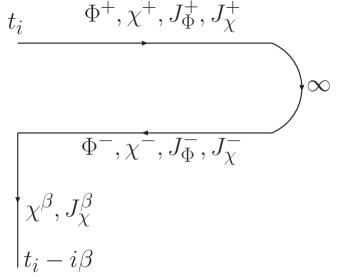
Figure 1: Contour in time for the non-equilibrium path integral representation.

The linear term $h\Phi^{\pm}$ is a counterterm that will be required to cancel the linear terms (tadpole) in $\Phi^{\pm}$ in the non-equilibrium effective action. This issue will be discussed below when we obtain the non-equilibrium effective action for the field $\Phi$ after integrating out the field(s) $\chi$.

The trace over the degrees of freedom of the $\chi$ field with the initial equilibrium density matrix, entail periodic (for bosons) or antiperiodic (for fermions) boundary conditions for $\chi$ along the contour $\mathcal{C}$. However, the boundary conditions on the path integrals for the field $\Phi$ are given by

$$\Phi^{+}(\vec{x},t=\infty)=\Phi^{-}(\vec{x},t=\infty)$$ (10)

and

$$\Phi^{+}(\vec{x},t=t_{i})=\Phi_{i}(\vec{x})\;\;\;;\;\;\;\Phi^{-}(\vec{x},t=t_{i})=\Phi^{\prime}_{i}(\vec{x})$$ (11)

The reason for the different path integrations is that whereas the $\chi$ field is traced over with an initial thermal density matrix (since it is taken as the “bath”), the initial density matrix for the $\Phi$ field will be specified later as part of the initial value problem. The path integral over $\chi$ leads to the influence functional for $\Phi^{\pm}$feyver .

II.1 Tracing over the “bath” degrees of freedom

As far as the path integrals over the bath degrees of freedom $\chi$ is concerned the fields $\Phi^{\pm}$ are simply c-number sources. The contour path integral

$$Z[\Phi^{\pm}]=\int{\cal D}\chi^{\pm}{\cal D}\chi^{\beta}e^{i\int_{\mathcal{C}}d^{4}x\Bigg{\{}\mathcal{L}_{\chi}(\chi)+J_{\chi}\chi+g\,\Phi\,\mathcal{O}[\chi]\Bigg{\}}}$$ (12)

is the generating functional of correlation functions of the field $\chi$ in presence of external c-number sources $\Phi^{\pm}$ (the sources $J^{\pm}_{\chi}$ generate the correlation functions via functional derivatives and are set to zero at the end of the calculation), namely

$$\int{\cal D}\chi^{\pm}{\cal D}\chi^{\beta}e^{i\int_{\mathcal{C}}d^{4}x\Big{\{}\mathcal{L}_{\chi}(\chi)+g\Phi\,\mathcal{O}[\chi]\Big{\}}}=\Big{\langle}e^{ig\int_{\mathcal{C}}d^{4}x\Phi\,\mathcal{O}[\chi]}\Big{\rangle}_{\chi}\,Z[0].$$ (13)

Note that the expectation value in the right hand side of eqn. (13) is in the equilibrium density matrix of the field $\chi$. The path integral can be carried out in perturbation theory and the result exponentiated to yield the effective action as follows

$$\Big{\langle}e^{ig\int_{\mathcal{C}}d^{4}x\Phi\,\mathcal{O}[\chi]}\Big{\rangle}_{\chi}=1+ig\int_{\mathcal{C}}d^{4}x\Phi(x)\,\Big{\langle}\mathcal{O}[\chi](x)\Big{\rangle}_{\chi}+\frac{(ig)^{2}}{2}\int_{\mathcal{C}}d^{4}x\int_{\mathcal{C}}d^{4}x^{\prime}\Phi(x)\Phi(x^{\prime})\Big{\langle}\mathcal{O}[\chi](x)\mathcal{O}[\chi](x^{\prime})\Big{\rangle}_{\chi}+\mathcal{O}(g^{3})$$ (14)

This the usual expansion of the exponential of the connected correlation functions, where this series is identified with

$$\Big{\langle}e^{ig\int_{\mathcal{C}}d^{4}x\Phi\,\mathcal{O}[\chi]}\Big{\rangle}_{\chi}=e^{i\,L_{if}[\Phi^{+},\Phi^{-}]}\;,$$ (15)

and where the influence functionalfeyver $L_{if}[\Phi^{+},\Phi^{-}]$ is given by the following expression

$$L_{if}[\Phi^{+},\Phi^{-}]=g\int_{\mathcal{C}}d^{4}x\Phi(x)\,\langle\mathcal{O}[\chi](x)\rangle_{\chi}+i\frac{g^{2}}{2}\int_{\mathcal{C}}d^{4}x\int_{\mathcal{C}}d^{4}x^{\prime}\Phi(x)\Phi(x^{\prime})\langle\mathcal{O}[\chi](x)\mathcal{O}[\chi](x^{\prime})\rangle_{\chi,con}+\mathcal{O}(g^{3})$$ (16)

In detail, the integrals along the contour $\mathcal{C}$ stand for the following:

$$\int_{\mathcal{C}}d^{4}x\Phi(x)\,\langle\mathcal{O}[\chi](x)\rangle_{\chi}=\int d^{3}x\int_{t_{i}}^{\infty}dt\left[\Phi^{+}(\vec{x},t)\langle\mathcal{O}[\chi^{+}](x)\rangle_{\chi}-\Phi^{-}(\vec{x},t)\langle\mathcal{O}[\chi^{-}](x)\rangle_{\chi}\right]$$ (17)

$$\int_{\mathcal{C}}d^{4}x\int_{\mathcal{C}}d^{4}x^{\prime}\Phi(x)\Phi(x^{\prime})\langle\mathcal{O}[\chi](x)\mathcal{O}[\chi](x^{\prime})\rangle_{\chi,con}= \int d^{3}x\int_{t_{i}}^{\infty}dt\int d^{3}x^{\prime}\int_{t_{i}}^{\infty}dt^{\prime}\Big{[}\Phi^{+}(x)\Phi^{+}(x^{\prime})\langle\mathcal{O}[\chi^{+}](x)\mathcal{O}[\chi^{+}](x^{\prime})\rangle_{\chi,con}$$

$$+ \Phi^{-}(x)\Phi^{-}(x^{\prime})\langle\mathcal{O}[\chi^{-}](x)\mathcal{O}[\chi^{-}](x^{\prime})\rangle_{\chi,con}$$

$$- \Phi^{+}(x)\Phi^{-}(x^{\prime})\langle\mathcal{O}[\chi^{+}](x)\mathcal{O}[\chi^{-}](x^{\prime})\rangle_{\chi,con}$$

$$- \Phi^{-}(x)\Phi^{+}(x^{\prime})\langle\mathcal{O}[\chi^{-}](x)\mathcal{O}[\chi^{+}](x^{\prime})\rangle_{\chi,con}\Big{]}$$ (18)

Since the expectation values above are computed in a thermal equilibrium translational invariant density matrix, it is convenient to introduce the spatial Fourier transform of the composite operator ${\cal O}$ in a spatial volume $V$ as

$${\cal O}_{\vec{k}}(t)=\frac{1}{\sqrt{V}}\int d^{3}xe^{i\vec{k}\cdot\vec{x}}{\cal O}[\chi(\vec{x},t)]$$ (19)

in terms of which we obtain following the correlation functions

$$\langle{\cal O}_{\vec{k}}(t)\rangle=\langle{\cal O}^{+}_{\vec{k}}(t)\rangle=\langle{\cal O}^{-}_{\vec{k}}(t)\rangle=\mathrm{Tr}\,e^{-\beta\,H_{\chi}}\,{O}_{\vec{k}}(t)$$ (20)

$$\langle{\cal O}_{\vec{k}}(t){\cal O}_{-\vec{k}}(t^{\prime})\rangle=\langle\mathcal{O}^{-}_{\vec{k}}(t){\cal O}^{+}_{-\vec{k}}(t^{\prime})\rangle=\mathrm{Tr}\,{\cal O}_{-\vec{k}}(t^{\prime})\,e^{-\beta\,H_{\chi}}\,{O}_{\vec{k}}(t)=\mathcal{G}^{>}_{k}(t-t^{\prime})={\cal G}^{-+}_{k}(t,t^{\prime})$$ (21)

$$\langle{\cal O}_{-\vec{k}}(t^{\prime}){\cal O}_{\vec{k}}(t)\rangle=\langle{\cal O}^{+}_{\vec{k}}(t){\cal O}^{-}_{-\vec{k}}(t^{\prime})\rangle=\mathrm{Tr}\,{O}_{\vec{k}}(t)\,e^{-\beta\,H_{\chi}}\,{\cal O}_{-\vec{k}}(t^{\prime})={\cal G}^{<}_{k}(t-t^{\prime})={\cal G}^{+-}_{k}(t,t^{\prime})={\cal G}^{-+}_{k}(t^{\prime},t)$$ (22)

$$\langle T{\cal O}_{\vec{k}}(t){\cal O}_{-\vec{k}}(t^{\prime})\rangle={\cal G}^{>}_{k}(t-t^{\prime})\Theta(t-t^{\prime})+{\cal G}^{<}_{k}(t-t^{\prime})\Theta(t^{\prime}-t)={\cal G}^{++}_{k}(t,t^{\prime})$$ (23)

$$\langle\widetilde{T}{\cal O}_{\vec{k}}(t){\cal O}_{-\vec{k}}(t^{\prime})\rangle={\cal G}^{>}_{k}(t-t^{\prime})\Theta(t^{\prime}-t)+{\cal G}^{<}_{k}(t-t^{\prime})\Theta(t-t^{\prime})={\cal G}^{--}_{k}(t,t^{\prime})$$ (24)

The time evolution of the operators is determined by the Heisenberg picture of $H_{\chi}$, namely ${\cal O}_{\vec{k}}(t)=e^{iH_{\chi}(t-t_{i})}{\cal O}_{\vec{k}}(t_{i})e^{-iH_{\chi}(t-t_{i})}$. Because the density matrix for the bath is in equilibrium, the correlation functions above are solely functions of the time difference. These correlation functions are computed exactly to all orders in the couplings of the bath fields amongst themselves.

These correlation functions are not independent, but obey

$$\mathcal{G}^{++}_{k}(t,t^{\prime})+\mathcal{G}^{--}_{k}(t,t^{\prime})-\mathcal{G}^{-+}_{k}(t,t^{\prime})-\mathcal{G}^{+-}_{k}(t,t^{\prime})=0$$ (25)

The non-equilibrium effective action is given by

$$L_{eff}[\Phi^{+},\Phi^{-}]=\int_{t_{i}}^{\infty}dtd^{3}x\,\left[\mathcal{L}_{0,\Phi}(\Phi^{+})+h\Phi^{+}-\mathcal{L}_{0,\Phi}(\Phi^{-})-h\Phi^{-}\right]+L_{if}[\Phi^{+},\Phi^{-}]$$ (26)

where we have set the sources $J^{\pm}$ for the fields $\Phi^{\pm}$ to zero.

The choice of counterterm

$$h=-\langle{\cal O}(\vec{x},t)\rangle$$ (27)

cancels the terms linear in $\Phi^{\pm}$ (tadpole) in the non-equilibrium effective action.

In what follows we take $t_{i}=0$ without loss of generality since (i) for $t>t_{i}$ the total Hamiltonian is time independent and the correlations will be solely functions of $t-t_{i}$, and (ii) we will be ultimately interested in the limit $t\gg t_{i}$ when all transient phenomena has relaxed. In terms of the spatial Fourier transform of the fields $\Phi^{\pm}$ defined as in eqn. (19) we find

$$iL_{eff}[\Phi^{+},\Phi^{-}] = \sum_{\vec{k}}\Bigg{\{}\frac{i}{2}\int_{0}^{\infty}dt\left[\dot{\Phi}^{+}_{\vec{k}}(t)\dot{\Phi}^{+}_{-\vec{k}}(t)-(k^{2}+m^{2})\Phi^{+}_{\vec{k}}(t)\Phi^{+}_{-\vec{k}}(t)-\dot{\Phi}^{-}_{\vec{k}}(t)\dot{\Phi}^{-}_{-\vec{k}}(t)+(k^{2}+m^{2})\Phi^{-}_{\vec{k}}(t)\Phi^{-}_{-\vec{k}}(t)\right]$$ (28)

$$-\frac{g^{2}}{2}\int_{0}^{\infty}dt\int_{0}^{\infty}dt^{\prime}\left[\Phi^{+}_{\vec{k}}(t){\cal G}^{++}_{k}(t,t^{\prime})\Phi^{+}_{-\vec{k}}(t^{\prime})+\Phi^{-}_{\vec{k}}(t){\cal G}^{--}_{k}(t,t^{\prime})\Phi^{-}_{-\vec{k}}(t^{\prime})\right.$$

$$\left.-\Phi^{+}_{\vec{k}}(t){\cal G}^{+-}_{k}(t,t^{\prime})\Phi^{-}_{-\vec{k}}(t^{\prime})-\Phi^{-}_{\vec{k}}(t){\cal G}^{-+}_{k}(t,t^{\prime})\Phi^{+}_{-\vec{k}}(t^{\prime})\right]\Bigg{\}}$$

where all the time integrations are in the interval $0\leq t\leq\infty$.

A similar program has been used recently to study the relaxation of scalar fieldsyokoyama as well as the photon production from a quark gluon plasma in thermal equilibriumboyphoton .

II.2 Stochastic description: generalized Langevin equation.

As it will become clear below, it is more convenient to introduce the Wigner center of mass and relative variables

$$\Psi(\vec{x},t)=\frac{1}{2}\left(\Phi^{+}(\vec{x},t)+\Phi^{-}(\vec{x},t)\right)\;\;;\;\;R(\vec{x},t)=\left(\Phi^{+}(\vec{x},t)-\Phi^{-}(\vec{x},t)\right)$$ (29)

and the Wigner transform of the initial density matrix for the $\Phi$ field

$${\cal W}(\Psi_{i};\Pi_{i})=\int DR_{i}e^{-i\int d^{3}x\Pi_{i}(\vec{x})R_{i}(\vec{x})}\rho(\Psi_{i}+\frac{R_{i}}{2};\Psi_{i}-\frac{R_{i}}{2})~{}~{};~{}~{}\rho(\Psi_{i}+\frac{R_{i}}{2};\Psi_{i}-\frac{R_{i}}{2})=\int D\Pi_{i}e^{i\int d^{3}x\Pi_{i}(\vec{x})R_{i}(\vec{x})}{\cal W}(\Psi_{i};\Pi_{i})$$ (30)

The boundary conditions on the $\Phi$ path integral given by (11) translate into the following boundary conditions on the center of mass and relative variables

$$\Psi(\vec{x},t=0)=\Psi_{i}\;\;;\;\;R(\vec{x},t=0)=R_{i}$$ (31)

furthermore, the boundary condition (10) yields the following boundary condition for the relative field

$$R(\vec{x},t=\infty)=0.$$ (32)

This observation will be important in the steps that follow. In terms of the spatial Fourier transforms of the center of mass and relative variables (29) introduced above, integrating by parts and accounting for the boundary conditions (31), the non-equilibrium effective action (28) becomes:

$$iL_{eff}[\Psi,R] = \int_{0}^{\infty}dt\sum_{\vec{k}}\left\{-iR_{-\vec{k}}\left(\ddot{\Psi}_{\vec{k}}(t)+(k^{2}+m^{2})\Psi_{k}(t)\right)\right\}$$ (33)

$$- \int_{0}^{\infty}dt\int_{0}^{\infty}dt^{\prime}\left\{\frac{1}{2}R_{-\vec{k}}(t)R_{\vec{k}}(t^{\prime}){\cal K}_{k}(t-t^{\prime})+R_{-\vec{k}}(t)i\Sigma^{R}_{k}(t-t^{\prime})\Psi_{\vec{k}}(t^{\prime})\right\}$$

$$+ \int d^{3}xR_{i}(\vec{x})\dot{\Psi}(\vec{x},t=0)$$

where the last term arises after the integration by parts in time, using the boundary conditions (31) and (32). The kernels in the above effective Lagrangian are given by (see eqns. (21-24))

$$\mathcal{K}_{k}(t-t^{\prime}) = \frac{g^{2}}{2}\left[{\cal G}_{k}^{>}(t-t^{\prime})+{\cal G}_{k}^{<}(t-t^{\prime})\right]$$ (34)

$$i\Sigma^{R}_{k}(t-t^{\prime}) = g^{2}\left[{\cal G}_{k}^{>}(t-t^{\prime})-{\cal G}_{k}^{<}(t-t^{\prime})\right]\Theta(t-t^{\prime})\equiv i\Sigma_{k}(t-t^{\prime})\Theta(t-t^{\prime})$$ (35)

The term quadratic in the relative variable $R$ can be written in terms of a stochastic noise as

$$\exp\Big{\{}-\frac{1}{2}\int dt\int dt^{\prime}R_{-\vec{k}}(t){\cal K}_{k}(t-t^{\prime})R_{\vec{k}}(t^{\prime})\Big{\}}=\int{\cal D}\xi\exp\Big{\{}-\frac{1}{2}\int dt\int dt^{\prime}~{}~{}\xi_{\vec{k}}(t){\cal K}^{-1}_{k}(t-t^{\prime})\xi_{-\vec{k}}(t^{\prime})$$

$$+i\int dt~{}~{}\xi_{-\vec{k}}(t)R_{\vec{k}}(t)\Big{\}}$$ (36)

The non-equilibrium generating functional can now be written in the following form

$${\cal Z} = \int D\Psi_{i}\int D\Pi_{i}\int{\cal D}\Psi{\cal D}R{\cal D}\xi~{}~{}{\cal W}(\Psi_{i};\Pi_{i})DR_{i}e^{i\int d^{3}xR_{i}(\vec{x})\left(\Pi_{i}(\vec{x})-\Psi(\vec{x},t=0)\right)}{\cal P}[\xi]$$

$$\exp\left\{-i\int_{0}^{\infty}dt~{}~{}R_{-\vec{k}}(t)\left[\ddot{\Psi}_{\vec{k}}(t)+(k^{2}+m^{2})\Psi_{\vec{k}}(t)+\int dt^{\prime}~{}~{}\Sigma^{R}_{k}(t-t^{\prime})\Psi_{\vec{k}}(t^{\prime})-\xi_{\vec{k}}(t)\right]\right\}$$

$${\cal P}[\xi] = \exp\left\{-\frac{1}{2}\int_{0}^{\infty}dt\int_{0}^{\infty}dt^{\prime}~{}~{}\xi_{\vec{k}}(t){\cal K}_{k}^{-1}(t-t^{\prime})\xi_{-\vec{k}}(t^{\prime})\right\}$$ (38)

The functional integral over $R_{i}$ can now be done, resulting in a functional delta function, that fixes the boundary condition $\dot{\Psi}(\vec{x},t=0)=\Pi_{i}(\vec{x})$.

Finally the path integral over the relative variable can be performed, leading to a functional delta function and the final form of the generating functional given by

$${\cal Z}=\int D\Psi_{i}D\Pi_{i}~{}~{}{\cal W}(\Psi_{i};\Pi_{i}){\cal D}\Psi{\cal D}\xi~{}~{}{\cal P}[\xi]\,\delta\left[\ddot{\Psi}_{\vec{k}}(t)+(k^{2}+m^{2})\Psi_{\vec{k}}(t)+\int_{0}^{t}dt^{\prime}~{}\Sigma_{k}(t-t^{\prime})\Psi_{\vec{k}}(t^{\prime})-\xi_{\vec{k}}(t)\right]$$ (39)

with the boundary conditions on the path integral on $\Psi$ given by

$$\Psi(\vec{x},t=0)=\Psi_{i}(\vec{x})\;\;;\;\;\dot{\Psi}(\vec{x},t=0)=\Pi_{i}(\vec{x})$$ (40)

where we have used the definition of $\Sigma^{R}_{k}(t-t^{\prime})$ in terms of $\Sigma_{k}(t-t^{\prime})$ given in equation (35).

The meaning of the above generating functional is the following: in order to obtain correlation functions of the center of mass Wigner variable $\Psi$ we must first find the solution of the classical stochastic Langevin equation of motion

$$\ddot{\Psi}_{\vec{k}}(t)+(k^{2}+m^{2})\Psi_{\vec{k}}(t)+\int_{0}^{t}dt^{\prime}~{}\Sigma_{k}(t-t^{\prime})\Psi_{\vec{k}}(t^{\prime})=\xi_{\vec{k}}(t)$$

$$\Psi_{\vec{k}}(t=0)=\Psi_{i,\vec{k}};~{}~{}\dot{\Psi}_{\vec{k}}(t=0)=\Pi_{i,\vec{k}}$$ (41)

for arbitrary noise term $\xi$ and then average the products of $\Psi$ over the stochastic noise with the Gaussian probability distribution ${\cal P}[\xi]$ given by (38), and finally average over the initial configurations $\Psi_{i}(\vec{x});\Pi_{i}(\vec{x})$ weighted by the Wigner function ${\cal W}(\Psi_{i},\Pi_{i})$, which plays the role of an initial phase space distribution function.

Calling the solution of (41) $\Psi_{\vec{k}}(t;\xi;\Psi_{i};\Pi_{i})$, the two point correlation function, for example, is given by

$$\langle\Psi_{-\vec{k}}(t)\Psi_{\vec{k}}(t^{\prime})\rangle=\int{\cal D}[\xi]{\cal P}[\xi]\int D\Psi_{i}\int D\Pi_{i}~{}~{}{\cal W}(\Psi_{i};\Pi_{i})\Psi_{\vec{k}}(t;\xi;\Psi_{i};\Pi_{i})\Psi_{-\vec{k}}(t^{\prime};\xi;\Psi_{i};\Pi_{i})$$ (42)

We note that in computing the averages and using the functional delta function to constrain the configurations of $\Psi$ to the solutions of the Langevin equation, there is the Jacobian of the operator $d^{2}/dt^{2}+(k^{2}+m^{2})+\int dt^{\prime}\Sigma^{ret}_{k}(t-t^{\prime})$ which however, is independent of the field and cancels between numerator and denominator in the averages.

This formulation establishes the connection with a stochastic problem and is similar to the Martin-Siggia-RoseMSR path integral formulation for stochastic phenomena. There are two different averages:

• The average over the stochastic noise term, which up to this order is Gaussian. We denote the average of a functional $\mathcal{F}[\xi]$ over the noise with the probability distribution function $P[\xi]$ given by eqn. (38) as

  $$\langle\langle\mathcal{F}[\xi]\rangle\rangle\equiv\frac{\int\mathcal{D}\xi P[\xi]\mathcal{F}[\xi]}{\int\mathcal{D}\xi P[\xi]}.$$ (43)

  Since the noise probability distribution function is Gaussian the only necessary correlation functions for the noise are given by

  $$\langle\langle\xi_{\vec{k}}(t)\rangle\rangle=0\;,\;\langle\langle\xi_{\vec{k}}(t)\xi_{\vec{k}^{\prime}}(t^{\prime})\rangle\rangle={\mathcal{K}}_{k}(t-t^{\prime})\,\delta^{3}(\vec{k}+\vec{k}^{\prime})$$ (44)

  and the higher order correlation functions are obtained from Wick’s theorem. Because the noise kernel $\mathcal{K}_{k}(t-t^{\prime})\neq\delta(t-t^{\prime})$ the noise is colored.

• The average over the initial conditions with the Wigner distribution function ${\cal W}(\Psi_{i},\Pi_{i})$ which we denote as

  $$\overline{\mathcal{A}[\Psi_{i},\Pi_{i}]}\equiv\frac{\int D\Psi_{i}\int D\Pi_{i}~{}~{}{\cal W}(\Psi_{i};\Pi_{i})\mathcal{A}[\Psi_{i},\Pi_{i}]}{\int D\Psi_{i}\int D\Pi_{i}~{}~{}{\cal W}(\Psi_{i};\Pi_{i})}$$ (45)

  In what follows we will consider a Gaussian initial Wigner distribution function with vanishing mean values of $\Psi_{i};\Pi_{i}$ with the following averages:

  $$\overline{\Psi_{i,\vec{k}}\Psi_{i,-\vec{k}}}=\frac{1}{2W_{k}}\left[1+2\mathcal{N}_{b,k}\right]$$ (46)

  $$\overline{\Pi_{i,\vec{k}}\Pi_{i,-\vec{k}}}=\frac{W_{k}}{2}\left[1+2\mathcal{N}_{b,k}\right]$$ (47)

  $$\overline{\Pi_{i,\vec{k}}\Psi_{i,-\vec{k}}+\Psi_{i,\vec{k}}\Pi_{i,-\vec{k}}}=0$$ (48)

  where $W_{k}$ is a reference frequency. Both $W_{k}$ and $\mathcal{N}_{b,k}$ characterize the initial gaussian density matrix. Such a density matrix describes a free field theory of particles with frequencies $W_{k}$. The averages (46,47) are precisely the expectation values obtained in a free field Fock state with $\mathcal{N}_{b,k}$ number of free field quanta of momentum $k$ and frequency $W_{k}$ or a free field density matrix which is diagonal in the Fock representation of a free field with frequency $W_{k}$. This can be seem simply by writing the field and canonical momentum in terms of the usual creation and annihilation operators of Fock quanta of momentum $k$ and frequency $W_{k}$. While this is a particular choice of initial state, we will see below that the distribution function becomes insensitive to it after a time scale longer than the quasiparticle relaxation time.

The average in the time evolved full density matrix is therefore defined by

$$\langle\cdots\rangle\equiv\overline{\langle\langle\cdots\rangle\rangle}~{}~{}.$$ (49)

II.3 Fluctuation and Dissipation:

From the expression (35) for the self-energy and the Wightmann functions (21,22) which are obtained as averages in the equilibrium density matrix of the $\chi$ fields (bath), we now obtain a dispersive representation for the kernels $\mathcal{K}_{k}(t-t^{\prime});\Sigma^{R}_{k}(t-t^{\prime})$. This is achieved by explicitly writing the expectation value in terms of energy eigenstates of the bath, introducing the identity in this basis, and using the time evolution of the Heisenberg field operators to obtain

$$g^{2}{\cal G}_{k}^{>}(t-t^{\prime}) = \int^{\infty}_{-\infty}d\omega~{}\sigma^{>}_{\vec{k}}(\omega)~{}e^{i\omega(t-t^{\prime})}$$ (50)

$$g^{2}{\cal G}_{k}^{<}(t-t^{\prime}) = \int^{\infty}_{-\infty}d\omega~{}\sigma^{<}_{\vec{k}}(\omega)~{}e^{i\omega(t-t^{\prime})}$$ (51)

with the spectral functions

$$\sigma^{>}_{\vec{k}}(\omega) = \frac{g^{2}}{\mathcal{Z}_{b}}\sum_{m,n}e^{-\beta E_{n}}\langle n|{\cal O}_{\vec{k}}(0)|m\rangle\langle m|{\cal O}_{-\vec{k}}(0)|n\rangle\,\delta(\omega-(E_{n}-E_{m}))$$ (52)

$$\sigma^{<}_{\vec{k}}(\omega) = \frac{g^{2}}{\mathcal{Z}_{b}}\sum_{m,n}e^{-\beta E_{m}}\langle n|{\cal O}_{-\vec{k}}(0)|m\rangle\langle m|{\cal O}_{\vec{k}}(0)|n\rangle\,\delta(\omega-(E_{m}-E_{n}))$$ (53)

where $\mathcal{Z}_{b}=\mathrm{Tr}\,e^{-\beta H_{\chi}}$ is the equilibrium partition function of the “bath”. Upon relabelling $m\leftrightarrow n$ in the sum in the definition (53) we find the KMS relationkapusta ; lebellac

$$\sigma^{<}_{k}(\omega)=\sigma^{>}_{k}(-\omega)=e^{\beta\omega}\sigma^{>}_{k}(\omega)$$ (54)

where we have used parity and rotational invariance in the second line above to assume that the spectral functions only depend of the absolute value of the momentum.

Using the spectral representation of the $\Theta(t-t^{\prime})$ we find the following representation for the retarded self-energy

$$\Sigma^{R}_{k}(t-t^{\prime})=\int_{-\infty}^{\infty}\frac{dk_{0}}{2\pi}e^{ik_{0}(t-t^{\prime})}\widetilde{\Sigma}^{R}(k,k_{0})$$ (55)

with

$$\widetilde{\Sigma}^{R}(k,k_{0})=\int_{-\infty}^{\infty}d\omega\frac{[\sigma^{>}_{k}(\omega)-\sigma^{<}_{k}(\omega)]}{\omega-k_{0}+i\epsilon}$$ (56)

Using the condition (54) the above spectral representation can be written in a more useful manner as

$$\widetilde{\Sigma}^{R}(k,k_{0}) = -\frac{1}{\pi}\int_{-\infty}^{\infty}d\omega\frac{\mathrm{Im}\widetilde{\Sigma}^{R}(k,\omega)}{\omega-k_{0}+i\epsilon}\,,$$ (57)

where the imaginary part of the self-energy is given by

$$\mathrm{Im}\widetilde{\Sigma}^{R}(k,\omega) = \pi\sigma^{>}_{k}(\omega)\left[e^{\beta\omega}-1\right]$$ (58)

and is clearly positive for $\omega>0$. Equation (54) entails that the imaginary part of the retarded self-energy is an odd function of frequency, namely

$$\mathrm{Im}\widetilde{\Sigma}^{R}(k,\omega)=-\mathrm{Im}\widetilde{\Sigma}^{R}(k,-\omega)\;.$$ (59)

The relation (58) leads to the following results which will be useful later

$$\sigma^{>}_{k}(\omega) = \frac{1}{\pi}\mathrm{Im}\widetilde{\Sigma}^{R}(k,\omega)\,n(\omega)$$ (60)

$$\sigma^{<}_{k}(\omega) = \frac{1}{\pi}\mathrm{Im}\widetilde{\Sigma}^{R}(k,\omega)\,\left[1+n(\omega)\right]$$ (61)

Similarly from the definitions (34) and (50,51) and the condition (54) we find

$$\mathcal{K}_{k}(t-t^{\prime}) = \int_{-\infty}^{\infty}\frac{dk_{0}}{2\pi}e^{ik_{0}(t-t^{\prime})}\widetilde{\mathcal{K}}(k,k_{0})$$ (62)

$$\widetilde{\mathcal{K}}(k,k_{0}) = \pi\sigma^{>}_{k}(k_{0})\left[e^{\beta k_{0}}+1\right]$$ (63)

whereupon using the condition (54) leads to the followint generalized form of the fluctuation-dissipation relation

$$\widetilde{\mathcal{K}}(k,k_{0})=\mathrm{Im}\widetilde{\Sigma}^{R}(k,k_{0})\coth\left[\frac{\beta k_{0}}{2}\right]$$ (64)

Thus we see that $\mathrm{Im}\widetilde{\Sigma}^{R}(k,k_{0})\,;\,\widetilde{\mathcal{K}}(k,k_{0})$ are odd and even functions of frequency respectively.

For further analysis below we will also need the following representation (see eqn. (35))

$$\Sigma_{k}(t-t^{\prime})=-i\int_{-\infty}^{\infty}e^{i\omega(t-t^{\prime})}\left[\sigma^{>}_{k}(\omega)-\sigma^{<}_{k}(\omega)\right]d\omega=\frac{i}{\pi}\int_{-\infty}^{\infty}e^{i\omega(t-t^{\prime})}\mathrm{Im}\widetilde{\Sigma}^{R}(k,\omega)d\omega$$ (65)

whose Laplace transform is given by

$$\widetilde{\Sigma}(k,s)\equiv\int^{\infty}_{0}dte^{-st}\Sigma_{k}(t)=-\frac{1}{\pi}\int^{\infty}_{-\infty}\frac{\mathrm{Im}\widetilde{\Sigma}^{R}(k,\omega)}{\omega+is}d\omega$$ (66)

This spectral representation, combined with (57) lead to the relation

$$\widetilde{\Sigma}^{R}(k,k_{0})=\widetilde{\Sigma}(k,s=ik_{0}+\epsilon)$$ (67)

We highlight that the self-energy $\widetilde{\Sigma}^{R}(k,k_{0})$ as well as the fluctuation kernel $\widetilde{\mathcal{K}}(k,k_{0})$ are to all orders in the couplings amongst the fields $\chi$ but to lowest order, namely $\mathcal{O}(g^{2})$ in the coupling between the field $\Phi$ and the fields $\chi$. The self-energy is depicted in fig.(2).

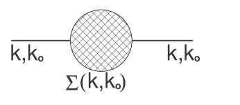
Figure 2: Self-energy of $\Phi$ to lowest order in $g^{2}$ but to all orders in the couplings of the fields $\chi$ amongst themselves. The external lines correspond to the field $\Phi$.

II.4 The solution:

The solution of the Langevin equation (41) can be found by Laplace transform. Defining the Laplace transforms

$$\widetilde{\Psi}_{\vec{k}}(s)\equiv\int^{\infty}_{0}dte^{-st}\Psi_{\vec{k}}(t)$$ (68)

$$\widetilde{\xi}_{\vec{k}}(s)\equiv\int^{\infty}_{0}dte^{-st}\xi_{\vec{k}}(t)$$ (69)

along with the Laplace transform of the self-energy given by eqn. (66) we find the solution

$$\widetilde{\Psi}_{\vec{k}}(s)=\frac{\Pi_{i,\vec{k}}+s\Psi_{i,\vec{k}}+\widetilde{\xi}_{\vec{k}}(s)}{s^{2}+\omega^{2}_{k}+\widetilde{\Sigma}(k,s)}~{}~{};~{}\omega^{2}_{k}=k^{2}+m^{2}$$ (70)

where we have used the initial conditions (40). The solution in real time can be written in a more compact manner as follows. Introduce the function $f_{k}(t)$ that obeys the following equation of motion and initial conditions

$$\ddot{f}_{k}(t)+\omega^{2}_{k}\,f_{k}(t)+\int_{0}^{t}dt^{\prime}~{}\Sigma_{k}(t-t^{\prime})f_{k}(t^{\prime})=0~{}~{};~{}~{}f(t=0)=0;~{}~{}\dot{f}_{k}(t=0)=1$$ (71)

whose Laplace transform is given by

$$\widetilde{f}_{k}(s)=\frac{1}{s^{2}+\omega^{2}_{k}+\widetilde{\Sigma}(k,s)}$$ (72)

In terms of this auxiliary function the solution of the Langevin equation (41) in real time is given by

$$\Psi_{k}(t;\Psi_{i};\Pi_{i};\xi)=\Psi_{i,\vec{k}}~{}\dot{f}_{k}(t)+\Pi_{i,\vec{k}}~{}f_{k}(t)+\int^{t}_{0}f_{k}(t-t^{\prime})~{}\xi_{\vec{k}}(t^{\prime})dt^{\prime}$$ (73)

For the study of the number operator below we will also need the time derivative of the solution, given by

$$\dot{\Psi}_{k}(t;\Psi_{i};\Pi_{i};\xi)=\Psi_{i,\vec{k}}~{}\ddot{f}_{k}(t)+\Pi_{i,\vec{k}}~{}\dot{f}_{k}(t)+\int^{t}_{0}\dot{f}_{k}(t-t^{\prime})~{}\xi_{\vec{k}}(t^{\prime})dt^{\prime}$$ (74)

where we have used the initial conditions given in eqn. (73). From eqn. (70) it is clear that the solution (73) represents a Dyson resummation of the perturbative expansion.

The real time solution for $f(t)$ is found by the inverse Laplace transform

$$f_{k}(t)=\int_{C}\frac{ds}{2\pi i}\frac{e^{st}}{s^{2}+\omega^{2}_{k}+\widetilde{\Sigma}(k,s)}$$ (75)

where $C$ stands for the Bromwich contour, parallel to the imaginary axis in the complex $s$ plane to the right of all the singularities of $\widetilde{f}(s)$ and along the semicircle at infinity for $\mathrm{Re}\,s<0$. The singularities of $\widetilde{f}(s)$ in the physical sheet are isolated single particle poles and multiparticle cuts along the imaginary axis. Thus the contour can be deformed to run parallel to the imaginary axis with a small positive real part with $s=i\omega+\epsilon\,;\,-\infty\leq\omega\leq\infty$ , returning parallel to the imaginary axis with $s=i\omega-\epsilon\,;\,\infty>\omega>-\infty$, with $\epsilon=0^{+}$ as depicted in fig. (3).

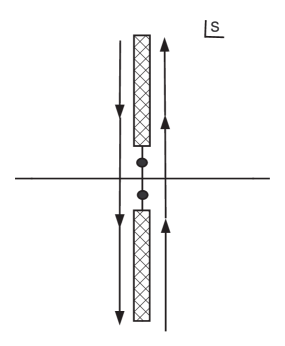
Figure 3: General structure of the self-energy in the complex s-plane. The dashed regions correspond to multiparticle cuts namely $\mathrm{Im}\widetilde{\Sigma}^{R}(k,s=i\omega+\epsilon)\neq 0$. The dots depict isolated poles.

From the spectral representations (58,66)) one finds that $\widetilde{\Sigma}(k,s=i\omega\pm\epsilon)=\mathrm{Re}\widetilde{\Sigma}^{R}(k,\omega)\pm\mathrm{Im}\widetilde{\Sigma}^{R}(k,\omega)$ and using that $\mathrm{Im}{\widetilde{\Sigma}}^{R}(k,\omega)=-\mathrm{Im}\widetilde{\Sigma}^{R}(k,-\omega)$ we find the following solution in real time

$$f_{k}(t)=\int_{-\infty}^{\infty}\sin(\omega t)\,\rho(k,\omega;T)\,d\omega\,,$$ (76)

where we have introduced the spectral density

$$\rho(k,\omega;T)=\frac{1}{\pi}\,\frac{~{}\left[\mathrm{Im}\widetilde{\Sigma}^{R}(k,\omega;T)+2\omega\epsilon\right]}{\left[\omega^{2}-\omega^{2}_{k}-\mathrm{Re}\widetilde{\Sigma}^{R}(k,\omega;T)\right]^{2}+\left[\mathrm{Im}\widetilde{\Sigma}^{R}(k,\omega;T)+2\omega\epsilon\right]^{2}}\;,$$ (77)

and we have made explicit the temperature dependence of the self-energy.

We have kept the infinitesimal $2\omega\epsilon$ with $\epsilon\rightarrow 0^{+}$ since if there are isolated single particle poles away from the multiparticle cuts for which $\mathrm{Im}\widetilde{\Sigma}^{R}(k,s)=0$ then this term ensures that the isolated pole contribution is accounted for, namely

$$\frac{1}{\pi}~{}\frac{2\omega\epsilon}{\left[\omega^{2}-\omega^{2}_{k}-\mathrm{Re}\widetilde{\Sigma}^{R}(k,\omega)\right]^{2}+\left[2\omega\epsilon\right]^{2}}=\mathrm{sign}(\omega)\,\delta\left[\omega^{2}-\omega^{2}_{k}-\mathrm{Re}\widetilde{\Sigma}^{R}(k,\omega)\right]\;.$$ (78)

The initial condition $\dot{f}_{k}(t=0)=1$ leads to the following sum rule

$$\int_{-\infty}^{\infty}\frac{d\omega}{\pi}~{}\frac{\omega\left[\mathrm{Im}\widetilde{\Sigma}^{R}(k,\omega)+2\omega\epsilon\right]}{\left[\omega^{2}-\omega^{2}_{k}-\mathrm{Re}\widetilde{\Sigma}^{R}(k,\omega)\right]^{2}+\left[\mathrm{Im}\widetilde{\Sigma}^{R}(k,\omega)+2\omega\epsilon\right]^{2}}=1$$ (79)

III Counting particles: the number operator

In an interacting theory the definition of a particle number requires careful consideration. To begin with, a distinction must be made between physical particles that appear in asymptotic states and can be counted by a detector, from unstable particles or resonances which have a finite lifetime and decay into other particles. Resonances are not asymptotic states, do not correspond to eigenstates of a Hamiltonian and their presence is inferred from virtual contributions to cross sections. In an interacting theory virtual processes turn a bare particle into a physical particle by dressing the bare particle with a cloud of virtual excitations. Physical particles correspond to asymptotic states and are eigenstates of the full (interacting) Hamiltonian with the physical mass. These physical particles correspond to real poles in the Green’s functions or propagators in the complex frequency plane. In the exact vacuum state, the propagator of the field associated with the physical particles features poles below the multiparticle continuum at the exact frequencies and with a residue given by the wave function renormalization constant $Z$. The wave function renormalization determines the overlap between the bare and interacting single particle states. Lorentz invariance of the vacuum state entails that the exact frequencies are of the form $\Omega_{k}=\sqrt{k^{2}+m^{2}_{P}}$, where $m_{P}$ is the physical mass and that the wave function renormalization is independent of the momentum $k$. In asymptotic theory, the spatial Fourier transform of the field operator $\hat{\Phi}_{\vec{k}}(t)$ obeys the (weak) asymptotic condition

$$\hat{\Phi}_{\vec{k}}(t)|0\rangle~{}~{}\overrightarrow{t\rightarrow\infty}~{}~{}\sqrt{\frac{Z}{{2\Omega_{k}}}}\,e^{i\Omega_{k}\,t}\,a^{\dagger}_{out}|0\rangle\equiv\sqrt{\frac{Z}{{2\Omega_{k}}}}\,e^{i\Omega_{k}\,t}\,|1_{\vec{k}}\rangle\,,$$ (80)

where $|1_{\vec{k}}\rangle$ is the state with one physical particle.

In a medium at finite temperature there are no asymptotic states, each particle, even when stable in vacuum acquires a width in a medium either by collisional processes (collisional broadening) or other processes such as Landau damping. The width acquired by a physical particle in a medium is a consequence of the interaction between the physical particle and the excitations in the medium. In particular the medium-induced width is necessary to ensure that physical particles relax to a state of thermal equilibrium with the medium. The relaxation rate is a measure of the width of the particle in the medium. Therefore in a medium a physical particle becomes a quasiparticle with a medium modification of the dispersion relation and a width.

Thus the question arises as to what particles are “counted” by a definition of a distribution function, namely, a decision must be made to count either physical particles or quasiparticles.

One can envisage counting physical particles by introducing a detector in the medium. Such detector must be calibrated so as to “click” every time it finds a particle with given characteristics. A detector that has been calibrated to measure physical particles in a scattering experiment for example, will measure the energy and the momentum (and any other good quantum numbers) of a particle. Every time that the detector measures a momentum $\vec{k}$ and an energy $\Omega_{k}$ determined by the dispersion relation of the physical particle (as well as other available quantum numbers), it counts this “hit” as one particle.

Once this detector has been calibrated in this manner, for example by carrying out a scattering experiment in the vacuum, we can insert this detector in a medium and let it count the physical particles in the medium.

Counting quasiparticles entails a different calibration of the detector which must account for the properties of the medium in the definition of a quasiparticle. The first obstacle in such calibration is the fact that a quasiparticle does not have a definite dispersion relation because its spectral density features a width, namely a quasiparticle is not associated with a sharp energy but with a continuum distribution of energies. How much of this distribution will be accepted by the detector in its definition of a quasiparticle, will depend on the filtering process involved in accepting a quasiparticle, and so cannot be unique. Therefore statements about measuring a distribution of quasiparticles are somewhat ambiguous.

In this article we focus on the first strategy, by counting only physical particles. Hence we propose a number operator that “counts” the physical particle states of mass $m_{P}$ that a detector will measure for example in a scattering experiment at asymptotically long times. Asymptotic theory and the usual reduction formula suggest the following definition of an interpolating number operator that counts the number of physical (stable) particles in a state

$$\hat{N}_{k}(t)=\frac{1}{2\Omega_{k}\,Z}\left\{\hat{\dot{\Phi}}_{\vec{k}}(t)\hat{\dot{\Phi}}_{-\vec{k}}(t)+\Omega^{2}_{k}\hat{{\Phi}}_{\vec{k}}(t)\hat{{\Phi}}_{-\vec{k}}(t)\right\}-\mathcal{C}_{k}$$ (81)

where $Z$ is the wave function renormalization, namely the residue of the single (physical) particle pole in the exact propagator, $\Omega_{k}=\sqrt{k^{2}+m^{2}_{P}}$ is the renormalized physical frequency and the normal ordering constant $\mathcal{C}_{k}$ will be adjusted so as to include renormalization effects. In free field theory $\Omega_{k}=\omega_{k}=\sqrt{k^{2}+m^{2}}\,,Z=1\,,\,\mathcal{C}_{k}=1/2$. However, in asymptotic theory the field $\Phi$ creates a single particle state of momentum $k$ and mass $m_{P}$ with amplitude $\sqrt{Z}$ out of the exact vacuum.

The quantity $\mathcal{C}_{k}$ arises from the necessity of redefining the normal ordering for the correct identification of the particle number in an interacting field theory. It will be fixed below by requiring that the expectation value of $\hat{N}_{k}(t)$ vanishes in the exact vacuum state at asymptotically long time. Alternatively this constant can be extracted from the equal time limit of the operator product expansion.

The approach that we follow is to consider an initial factorized density matrix corresponding to a tensor product of a density matrix of the field $\Phi$ and a thermal bath of the fields $\chi$. This initial state will evolve in time with the full interacting Hamiltonian, leading to transient phenomena which results in the dressing of the bare particles by the virtual excitations. At asymptotically long times the bare particle is fully dressed into the physical particle, and at finite temperature, a quasiparticle. The time evolution of the interpolating number operator will reflect this transient stage and the dynamics of the dressing of the bare into the physical state. Since the thermal bath is stationary, the distribution of physical particles in the bath will be extracted from the asymptotic long time limit of the expectation value of the interpolating Heisenberg number operator $\hat{N}_{k}(t)$ in the initial state.

The expectation value of $\hat{N}_{k}(t)$ is related to the real-time correlation functions of the field $\Phi$ as follows

$$\langle\hat{N}_{k}(t)\rangle=\frac{1}{4\Omega_{k}\,Z}\left(\frac{\partial}{\partial t}\frac{\partial}{\partial t^{\prime}}+\Omega^{2}_{k}\right)\Bigg{[}g^{>}_{k}(t,t^{\prime})+g^{<}_{k}(t,t^{\prime})\Bigg{]}_{t=t^{\prime}}-\mathcal{C}_{k}$$ (82)

where the non-equilibrium correlation functions are given by

$$\langle\Phi^{+}_{\vec{k}}(t)\Phi^{+}_{-\vec{k}}(t^{\prime})\rangle=g^{>}_{k}(t,t^{\prime})\Theta(t-t^{\prime})+g^{<}_{k}(t,t^{\prime})\Theta(t^{\prime}-t)$$ (83)

$$\langle\Phi^{-}_{\vec{k}}(t)\Phi^{-}_{-\vec{k}}(t^{\prime})\rangle=g^{>}_{k}(t,t^{\prime})\Theta(t^{\prime}-t)+g^{<}_{k}(t,t^{\prime})\Theta(t-t^{\prime})$$ (84)

$$\langle\Phi^{-}_{\vec{k}}(t)\Phi^{+}_{-\vec{k}}(t^{\prime})\rangle=g^{>}_{k}(t,t^{\prime})$$ (85)

$$\langle\Phi^{-}_{-\vec{k}}(t^{\prime})\Phi^{+}_{\vec{k}}(t)\rangle=g^{<}_{k}(t,t^{\prime})$$ (86)

The symmetrized definition of the expectation value (82) has been chosen for convenience because, as it is shown in detail below, it is related to a simple correlation function of the center of mass field $\Psi_{k}(t)$ given by eqn. (29). However we could have chosen any other definition of the equal time correlation function, such as $g^{>}_{k}(t,t);g^{<}_{k}(t,t)$ or any combination thereof that does not involve a Heaviside step function in time for which the time derivatives will yield spurious delta functions. It is a straightforward exercise with the density matrix to show that all of these alternative definitions are equivalent in the equal time limit, since these do not involve discontinuous functions of time.

In terms of the center of mass field $\Psi_{k}(t)=(\Phi^{+}_{\vec{k}}(t)+\Phi^{-}_{\vec{k}}(t))/2$ introduced above it is straightforward to find that the correlation function in the bracket in (82) is given by

$$\langle\Psi_{\vec{k}}(t)\Psi_{-\vec{k}}(t^{\prime})\rangle=\frac{1}{2}\left[g^{>}_{k}(t,t^{\prime})+g^{<}_{k}(t,t^{\prime})\right]$$ (87)

and the occupation number can be written in terms of the center of mass Wigner variable introduced in eqn. (29) as follows

$$\langle\hat{N}_{k}(t)\rangle=\frac{1}{2\Omega_{k}Z}\left[\langle\dot{\Psi}_{\vec{k}}(t)\dot{\Psi}_{-\vec{k}}(t)\rangle+\Omega^{2}_{k}\langle\Psi_{\vec{k}}(t)\Psi_{-\vec{k}}(t)\rangle\right]-\mathcal{C}_{k}$$ (88)

where the expectation values are obtained as in eqn. (49) and $\Psi_{\vec{k}}(t)$ is the solution of the Langevin equation given by (73,74).

A straightforward calculation implementing eqn. (49) writing the noise in terms of its temporal Fourier transform and using the Fourier representation of the noise kernel (62) leads to the following result

$$N_{k}(t)\equiv\langle\hat{N}_{k}(t)\rangle = \frac{1}{2\Omega_{k}Z}\left\{\frac{1}{2W_{k}}\left[1+2\mathcal{N}_{b,k}\right]\left[\ddot{f}^{2}_{k}(t)+(\Omega^{2}_{k}+W^{2}_{k})~{}\dot{f}^{2}_{k}(t)+\Omega^{2}_{k}W^{2}_{k}~{}f^{2}_{k}(t)\right]\right.$$ (89)

$$\left.+\int_{-\infty}^{\infty}\frac{d\omega}{2\pi}\widetilde{\cal K}(k,\omega)\left[|\mathcal{F}_{k}(\omega,t)|^{2}+\Omega^{2}_{k}|\mathcal{H}_{k}(\omega,t)|^{2}\right]\right\}-\mathcal{C}_{k}$$

where we have introduced

$$\mathcal{H}_{k}(\omega,t)=\int_{0}^{t}d\tau{f}_{k}(\tau)e^{-i\omega\tau}$$ (90)

$$\mathcal{F}_{k}(\omega,t)=\int_{0}^{t}d\tau\dot{f}_{k}(\tau)e^{-i\omega\tau}$$ (91)

$f_{k}(t)$ is given in eqn. (76) and the fluctuation kernel $\widetilde{\cal K}(k,\omega)$ is given by eqn. (64).

The result (89) for the time evolution of the distribution function, along with the expressions (90,91) clearly highlights the non-Markovian nature of the evolution. The integrals in time in (90,91) include memory of the past evolution. This is one of the most important aspects that distinguishes the quantum kinetic approach from the usual Boltzmann equation. We will contrast these aspects in section (V).

III.1 Counting physical particles in a thermal bath.

In the vacuum the spectral density of the field $\Phi$ which describes a physical particle is depicted in fig. (4). It features isolated poles along the real axis in the physical sheet in the complex frequency ($\omega$) plane at the position of the exact single particle dispersion relation $\Omega_{k}$ with $|\Omega_{k}|<|\omega_{th}|$ where $\omega_{th}$ is the lowest multiparticle threshold.

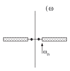
Figure 4: Spectral density $\rho_{k}(\omega,T=0)$ for stable particles. The dots represent the isolated poles at $\pm\Omega_{k}$ and the shaded regions the multiparticle cuts. $\omega_{th}$ is the lowest multiparticle threshold.

As mentioned above, in a medium stable physical particles acquire a width as a consequence of the interactions with physical excitations, and become quasiparticles. The width can originate in several different processes such as collisions or Landau damping. The poles move off the physical sheet into the second (or higher) Riemann sheet in the complex $\omega$ plane, thus becoming a resonance. This is the statement that there are no asymptotic states in the medium.

The analytic structure of the spectral density at finite temperature is in general fairly complicated. While at zero temperature the multiparticle thresholds are above the light cone $|\omega|>k$, at finite temperature (or density) there appear branch cuts with support below the light conekapusta ; lebellac ; weldon ; brapis . However a general statement in a medium is that the poles associated with stable particles in vacuum (along the real axis in the physical sheet) move off the physical sheet and the spectral density does not feature isolated poles but only branch cut singularities in the physical sheet, associated with multiparticle processes in the medium.

In perturbation theory the resonance is very close to the real axis (but in the second or higher Riemann sheet) and the width is very small as compared with the position of the resonance. We will study a particular example in the next section.

In perturbation theory the spectral density $\rho(k,\omega,T)$ (77) features a sharp peak at the position of the quasiparticle “pole” which is determined by

$$\mathcal{W}^{2}_{k}(T)-\omega^{2}_{k}-\mathrm{Re}\widetilde{\Sigma}^{R}(k,\mathcal{W}_{k}(T);T)=0$$ (92)

Near the quasiparticle “poles” the spectral density is well described by the Breit-Wigner approximation

$$\rho_{BW}(k,\omega;T)\simeq\frac{\mathcal{Z}_{k}(T)}{2\mathcal{W}_{k}(T)}~{}\frac{1}{\pi}\frac{\mathrm{sign}(\omega)\,\Gamma_{k}(T)}{(|\omega|-\mathcal{W}_{k}(T))^{2}+\Gamma^{2}_{k}(T)}\;,$$ (93)

where $\mathcal{W}_{k}(T)$ is determined by eqn. (92) and the finite temperature residue and width are given by

$$\frac{1}{\mathcal{Z}_{k}(T)}=\Bigg{[}1-\frac{1}{2\mathcal{W}_{k}(T)}\frac{\partial\mathrm{Re}\widetilde{\Sigma}^{R}(k,\omega;T)}{\partial\omega}\Bigg{]}_{\omega=\mathcal{W}_{k}(T)}$$ (94)

$$\Gamma_{k}(T)=\mathcal{Z}_{k}\frac{\mathrm{Im}\widetilde{\Sigma}^{R}(k,\mathcal{W}_{k}(T);T)}{2\mathcal{W}_{k}(T)}$$ (95)

At zero temperature of the bath, the (quasi) particle dispersion relation $\mathcal{W}_{k}(T)$ is identified with the dispersion relation of the stable physical particle, namely the “on-shell” pole, the residue $\mathcal{Z}_{k}(T)$ is identified with the wavefunction renormalization constant $Z$ which is the residue at the on-shell pole for the physical particle, and the width vanishes at zero temperature since the particle is stable in the vacuum, namely

$$\mathcal{W}_{k}(T=0) = \Omega_{k}$$ (96)

$$\mathcal{Z}_{k}(T=0) = Z$$ (97)

$$\Gamma_{k}(T=0) = 0$$ (98)

In the Breit-Wigner approximation the real time solution is easily found to be

$$f^{BW}_{k}(t)\simeq\mathcal{Z}_{k}(T)\frac{\sin\left[\mathcal{W}_{k}(T)\,t\right]}{\mathcal{W}_{k}(T)}\,e^{-\Gamma_{k}(T)\,t}$$ (99)

This solution describes the relaxation of single quasiparticles, where $\mathcal{W}_{k}(t)$ is the quasiparticle dispersion relation and $\Gamma_{k}(T)$ is the quasiparticle decay rate.

The asymptotic long time limit of the distribution function (89) is obtained by using the following identities

$${\cal H}_{k}(\omega,\infty)=\int_{0}^{\infty}e^{-i(\omega-i\epsilon)t}f_{k}(t)dt = \widetilde{f}_{k}(s=i\omega+\epsilon)$$ (100)

$${\cal F}_{k}(\omega,\infty)=\int_{0}^{\infty}e^{-i(\omega-i\epsilon)t}\dot{f}_{k}(t)dt = i\omega\widetilde{f}_{k}(s=i\omega+\epsilon)$$ (101)

where $\widetilde{f}_{k}(s)$ is the Laplace transform of $f_{k}(t)$ given by eqn. (72) and in (101) we have integrated by parts, used the initial condition $f_{k}(0)=0$ and introduced a convergence factor $\epsilon\rightarrow 0^{+}$. Hence the expectation value of the interpolating number operator in the asymptotic long-time limit is given by

$$N_{k}(\infty)=\int_{0}^{\infty}\Bigg{(}\frac{\omega^{2}+\Omega^{2}_{k}}{2\,Z\,\Omega_{k}}\Bigg{)}\left[1+2n(\omega)\right]\rho(k,\omega,T)\,{d\omega}\,-\mathcal{C}_{k}\;,$$ (102)

where $n(\omega)$ is the Bose-Einstein distribution function and we have used the fluctuation-dissipation relation (64) as well as eqn. (72) which lead to the $\rho(k,\omega,T)$ in (102). The dependence of the asymptotic distribution function on the spectral density is a consequence of the fluctuation-dissipation relation (64) as well as the non-Markovian time evolution as displayed in (100,101).

The real time solution (99) clearly reveals that the asymptotic limit is reached for $t>\tau_{k}=1/2\Gamma_{k}(T)$ where $\Gamma_{k}(T)$ is the quasiparticle relaxation rate. The distribution function at $t>>\tau_{k}$ does not depend on the initial distribution $\mathcal{N}_{b,k}$ or the reference frequencies $W_{k}$. Therefore at times longer than the quasiparticle relaxation time the distribution function becomes independent of the initial conditions. This is to be expected if the state reaches thermal equilibrium with the bath, since in thermal equilibrium there is no memory of the initial conditions or correlations.

The integral term in the asymptotic distribution (102) is easily understood as full thermalization from the following argument.

Let us consider the correlations functions $g^{>}_{k}(t,t^{\prime});g^{<}_{k}(t,t^{\prime})$ given by eqns. (85,86). In thermal equilibrium they have the spectral representation

$$g^{>}_{k}(t,t^{\prime}) = \int\rho^{>}(k,\omega;T)\,e^{i\omega(t-t^{\prime})}d\omega$$ (103)

$$g^{<}_{k}(t,t^{\prime}) = \int\rho^{<}(k,\omega;T)\,e^{i\omega(t-t^{\prime})}d\omega$$ (104)

where

$$\rho^{>}(k,\omega;T) = \frac{1}{\mathcal{Z}_{T}}\sum_{m,n}e^{-\beta E_{n}}\langle n|{\Phi}_{\vec{k}}(0)|m\rangle\langle m|{\Phi}_{-\vec{k}}(0)|n\rangle\,\delta(\omega-(E_{n}-E_{m}))$$ (105)

$$\rho^{<}(k,\omega;T) = \frac{1}{\mathcal{Z}_{T}}\sum_{m,n}e^{-\beta E_{m}}\langle n|{\Phi}_{-\vec{k}}(0)|m\rangle\langle m|{\Phi}_{\vec{k}}(0)|n\rangle\,\delta(\omega-(E_{m}-E_{n}))\,.$$ (106)

Where $\mathcal{Z}_{T}$ is the thermal equilibrium partition function. A straightforward re-labelling of indices leads to the relation

$$\rho^{<}(k,\omega;T)=\rho^{>}(k,-\omega;T)=e^{\beta\omega}\rho^{>}(k,\omega;T)$$ (107)

The spectral density is given by

$$\rho(k,\omega;T)=\rho^{<}(k,\omega;T)-\rho^{>}(k,\omega;T)$$ (108)

leading to the relations

$$\rho^{>}(k,\omega;T) = \rho(k,\omega;T)\,n(\omega)$$ (109)

$$\rho^{<}(k,\omega;T) = \rho(k,\omega;T)\,\left[1+n(\omega)\right]\,,$$ (110)

where $n(\omega)=1/[e^{\beta\omega}-1]$.

Therefore in thermal equilibrium the expectation value of the operator term in eqns. (81, 82) is given by

$$\frac{1}{4\Omega_{k}\,Z}\left(\frac{\partial}{\partial t}\frac{\partial}{\partial t^{\prime}}+\Omega^{2}_{k}\right)\Bigg{[}g^{>}_{k}(t,t^{\prime})+g^{<}_{k}(t,t^{\prime})\Bigg{]}_{t=t^{\prime}}=\int_{-\infty}^{\infty}\Bigg{(}\frac{\omega^{2}+\Omega^{2}_{k}}{4\,Z\,\Omega_{k}}\Bigg{)}\left[1+2n(\omega)\right]\,\rho(k,\omega;T)\,{d\omega}\,,$$ (111)

which is precisely the integral term in the asymptotic limit given by eqn. (102). Therefore the expression (102) indicates that the excitations of the field $\Phi$ have reached a state of thermal equilibrium with the bath. The normal ordering constant $\mathcal{C}_{k}$ in (102) is a subtraction necessary to redefine normal ordering in the interacting theory and is defined from the operator product expansion to yield vanishing number of particles in the vacuum.

While the asymptotic long time limit can be obtained directly from the spectral representation of the interpolating number operator in the equilibrium state, the real time formulation in terms of the non-equilibrium effective action has two advantages: i) it makes explicit the connection with the fluctuation dissipation relation and clearly states that the equilibrium abundance is determined by the noise correlation function of the bath, ii) the real time dynamics clearly shows thermalization on time scales $t>\tau_{k}$. These statements would not be immediately recognized from the equilibrium spectral representation.

The result (102) becomes more illuminating in the narrow width approximation where the Breit-Wigner approximation for the spectral density (93) is supplemented with the narrow width limit $\Gamma_{k}(T)\rightarrow 0$ which leads to

$$\rho(k,\omega;T)\simeq\frac{\mathcal{Z}_{k}(T)}{2\mathcal{W}_{k}(T)}~{}\mathrm{sign}(\omega)\delta\left(|\omega|-\mathcal{W}_{k}(T)\right)\;,$$ (112)

which in turn leads to the approximate result

$$N_{k}(\infty)\sim\frac{\mathcal{Z}_{k}(T)}{Z}\Bigg{(}\frac{\mathcal{W}^{2}_{k}(T)+\Omega^{2}_{k}}{2\,\mathcal{W}_{k}(T)\,\Omega_{k}}\Bigg{)}\left[\frac{1}{2}+n(\mathcal{W}_{k}(T))\right]-\mathcal{C}_{k}$$ (113)

Obviously the zero temperature pole $\Omega_{k}$ and residue $Z$ and their finite temperature counterparts $\mathcal{W}_{k}(T),\mathcal{Z}_{k}(T)$ differ by terms that are of order $g^{2}$, namely perturbatively small, therefore in the narrow width approximation, which itself is a result of the weak coupling assumption one could write

$$N_{k}(\infty)\sim n(\Omega_{k})+\left[\frac{1}{2}+\mathcal{O}(g^{2})-\mathcal{C}_{k}\right]$$ (114)

Thus choosing the normal ordering factor $\mathcal{C}_{k}=1/2+\mathcal{O}(g^{2})$ would lead to the conclusion that the physical particles are distributed in the thermal bath with a Bose-Einstein distribution function with the argument being the physical pole frequency (at zero temperature). Furthermore the normal ordering constant $\mathcal{C}_{k}\sim 1/2$ is identified with the usual normal ordering of the number operator in the free field vacuum.

In order to understand in detail the perturbative correction we have to first decide on what are $\Omega_{k},Z,\mathcal{C}_{k}$. The importance of the perturbative corrections cannot be underestimated, if the temperature of the bath is much smaller than $\Omega_{k}$ the distribution function $n(\Omega_{k})\ll 1$ and the perturbative corrections can be of the same order or larger. What should be clear from the above discussion is that in order to make precise the perturbative correction to the abundance, we must specify unambiguously what is being counted.

III.1.1 Physical particles in the vacuum

The next step is to define $\Omega_{k},Z,\mathcal{C}_{k}$. As it was emphasized above, the number operator that we seek counts physical particles. These are stable excitations off the full vacuum state of the theory and are associated with isolated single particle poles in the spectral density at zero temperature.

The zero temperature limit of the asymptotic distribution function (102) is

$$N_{k}(\infty;T=0)=\int_{0}^{\infty}\Bigg{(}\frac{\omega^{2}+\Omega^{2}_{k}}{2\,Z\,\Omega_{k}}\Bigg{)}\,\rho(k,\omega,T=0)\,{d\omega}-\mathcal{C}_{k}\;,$$ (115)

At $T=0$ the spectral density features the isolated single particle poles away from the multiparticle continuum as depicted in fig. (4). The contribution from the single particle poles to the zero temperature spectral density is given by eqn. (78), therefore we write

$$\rho(k,\omega,T=0)=\mathrm{sign}(\omega)\,\frac{Z}{2\Omega_{k}}\,\delta(\omega-\Omega_{k})+\rho_{c}(k,\omega,T=0)\,,$$ (116)

where $\rho_{c}(k,\omega,T=0)$ is the continuum contribution with support for $|\omega|>\omega_{th}$, where $\omega_{th}$ is the lowest multiparticle threshold, and the position of the isolated pole satisfies

$$\Omega^{2}_{k}-\omega^{2}_{k}-\mathrm{Re}\widetilde{\Sigma}^{R}(k,\Omega_{k})=0$$ (117)

At zero temperature Lorentz covariance implies that $\Omega^{2}_{k}=k^{2}+m^{2}_{P}$, where $m_{P}$ is the pole mass of the physical excitations (asymptotic states).

The residue at the single (physical) particle pole, $Z$, is given by

$$\frac{1}{Z}=\Bigg{[}1-\frac{1}{2\Omega_{k}}\frac{\partial\mathrm{Re}\widetilde{\Sigma}^{R}(k,\omega;T)}{\partial\omega}\Bigg{]}_{\omega=\Omega_{k}}\,.$$ (118)

Introducing the zero temperature form of the spectral density (116) in the sum rule (79) the following alternative expression is obtained.

$$Z=1-2\int_{\omega_{th}}^{\infty}\omega\,\rho_{c}(k,\omega,T=0)\,d\omega$$ (119)

Therefore the asymptotic distribution of particles in the vacuum is given by

$$N_{k}(\infty;T=0)=\frac{1}{2}+\int_{0}^{\infty}\Bigg{(}\frac{\omega^{2}+\Omega^{2}_{k}}{2\,Z\,\Omega_{k}}\Bigg{)}\,\rho_{c}(k,\omega,T=0)\,{d\omega}-\mathcal{C}_{k}\;,$$ (120)

The normal ordering term $\mathcal{C}_{k}$ is now fixed by requiring that for $T=0$ the vacuum state has vanishing number of physical excitations. In other words, by requiring $N_{k}(\infty,T=0)=0$ we are led to

$$\mathcal{C}_{k}=\frac{1}{2}+\int_{0}^{\infty}\Bigg{(}\frac{\omega^{2}+\Omega^{2}_{k}}{2\,Z\,\Omega_{k}}\Bigg{)}\,\rho_{c}(k,\omega,T=0)\,{d\omega}.$$ (121)

We have kept the lower limit in the integral to be $\omega=0$ for further convenience, however $\rho_{c}(k,\omega,T=0)$ vanishes for $|\omega|<\omega_{th}$.

Equations (117), (118,119) and (121) determine all of the parameters $\Omega_{k},Z,\mathcal{C}_{k}$ for the proper definition of the distribution function for physical particles.

Hence the distribution function of physical excitations in equilibrium with the bath at finite temperature is finally given by the simple expression

$$\mathcal{N}(k,T)\equiv N_{k}(\infty)=\int_{0}^{\infty}\Bigg{(}\frac{\omega^{2}+\Omega^{2}_{k}}{2\,Z\,\Omega_{k}}\Bigg{)}\Bigg{\{}\left[1+2n(\omega)\right]\rho(k,\omega,T)-\rho_{c}(k,\omega,T=0)\Bigg{\}}\,{d\omega}\,-\frac{1}{2}\;,$$ (122)

This is the final form of the asymptotic distribution function of physical particles in equilibrium in the thermal bath with $\Omega_{k}=\sqrt{k^{2}+m^{2}_{P}};Z;\mathcal{C}_{k}$ given by equations (117),(118) (or (119),(121)) respectively.

III.2 Renormalization:

In renormalizable theories the wavefunction renormalization constant $Z$ is ultraviolet divergent and the expression for the asymptotic distribution function (122) seems to be ambiguous. However proper renormalization as described below shows that the asymptotic abundance is finite.

In general the imaginary part of the self-energy can be written as a sum of a zero temperature and a finite temperature contribution, the latter vanishing at zero temperature, thus we write

$$\mathrm{Im}\widetilde{\Sigma}^{R}(\omega,k;T)=\mathrm{Im}\widetilde{\Sigma}^{R}_{0}(\omega,k)+\mathrm{Im}\widetilde{\Sigma}^{R}_{T}(\omega,k)$$ (123)

Therefore the real part of the self-energy, which is obtained from the imaginary part by a dispersion relation (Kramers-Kronig) can also be written as a sum of a zero temperature plus a finite temperature contribution,

$$\mathrm{Re}\widetilde{\Sigma}^{R}(\omega,k;T)=-\frac{1}{\pi}\mathcal{P}\int^{\infty}_{0}2k_{0}\frac{\mathrm{Im}\widetilde{\Sigma}^{R}(k_{0},k;T)}{k^{2}_{0}-\omega^{2}}~{}dk_{0}\equiv\mathrm{Re}\widetilde{\Sigma}^{R}_{0}(\omega,k)+\mathrm{Re}\widetilde{\Sigma}^{R}_{T}(\omega,k)$$ (124)

where $\mathcal{P}$ stands for the principal part of the integral, and we have used the fact that $\mathrm{Im}\widetilde{\Sigma}^{R}(k_{0},k;T)$ is an odd function of $k_{0}$. Both $\mathrm{Im}\widetilde{\Sigma}^{R}_{T}(\omega,k)$ and $\mathrm{Re}\widetilde{\Sigma}^{R}_{T}(\omega,k)$ vanish at $T=0$.

The position of the physical pole is obtained at zero temperature from the relation (117),

$$\Omega^{2}_{k}-\omega^{2}_{k}-\mathrm{Re}\widetilde{\Sigma}^{R}_{0}(k,\Omega_{k})=0$$ (125)

The subtracted real part of the self energy is

$$\mathrm{Re}\widetilde{\Sigma}^{R}_{0}(k,\omega)-\mathrm{Re}\widetilde{\Sigma}^{R}_{0}(k,\Omega_{k})=\Big{[}1-Z^{-1}[k,\omega]\Big{]}(\omega^{2}-\Omega^{2}_{k})$$ (126)

where

$$Z^{-1}[k,\omega]=1+\frac{1}{\pi}\mathcal{P}\int_{0}^{\infty}2k_{0}\frac{\mathrm{Im}\widetilde{\Sigma}^{R}_{0}(k_{0},k)}{(k_{0}^{2}-\omega^{2})(k^{2}_{0}-\Omega^{2}_{k})}~{}dk_{0}.$$ (127)

This expression for $Z^{-1}[k,\omega]$ follows from the zero temperature limit of the dispersive representation in eqn. (124).

The function $Z[k,\omega=\Omega_{k}]$, namely evaluated on the single particle mass shell, is identified with the wave function renormalization, or residue at the single particle pole at zero temperature.

As mentioned above, in renormalizable theories $Z[k,\omega]$ is ultraviolet logarithmically divergent, therefore it is convenient to perform yet another subtraction of the integral term in (127) as follows,

$$Z^{-1}[k,\omega]=Z^{-1}-\Pi_{0}(k,\omega)\,,$$ (128)

where $Z$ is the wavefunction renormalization constant, namely the residue at the pole,

$$Z^{-1}=1+\frac{1}{\pi}\mathcal{P}\int_{0}^{\infty}2k_{0}\frac{\mathrm{Im}\widetilde{\Sigma}^{R}_{0}(k_{0},k)}{(k^{2}_{0}-\Omega^{2}_{k})^{2}}~{}dk_{0}\,,$$ (129)

and $\Pi_{0}(k,\omega)$ is the real part of the twice subtracted self-energy given by

$$\Pi_{0}(k,\omega)=-\frac{1}{\pi}(\omega^{2}-\Omega^{2}_{k})~{}\mathcal{P}\int_{0}^{\infty}2k_{0}\frac{\mathrm{Im}\widetilde{\Sigma}^{R}_{0}(k_{0},k)}{(k_{0}^{2}-\omega^{2})(k^{2}_{0}-\Omega^{2}_{k})^{2}}~{}dk_{0}$$ (130)

The two subtractions had been performed on the single particle mass-shell. In a renormalizable theory the integral in the twice subtracted real part of the self energy $\Pi_{0}(k,\omega)$ is ultraviolet finite while the integral in $Z^{-1}$ is logarithmically divergent. Furthermore the finite temperature parts do not have primitive divergences since all the primitive divergences are those of the zero temperature theory. We emphasize that these expressions are still functions of the bare coupling and any potential divergences arising from coupling renormalization have not yet been accounted for. The divergences associated with coupling constant renormalization will be addressed below.

Combining equations (125), (126) and (128), the spectral density (77) can be written in the following form

$$\rho(k,\omega;T)=\frac{1}{\pi}\,\frac{~{}\left[\mathrm{Im}\widetilde{\Sigma}^{R}(k,\omega;T)+2\omega\epsilon\right]}{\left[Z^{-1}(\omega^{2}-\Omega^{2}_{k})-\widetilde{\Pi}(k,\omega;T)\right]^{2}+\left[\mathrm{Im}\widetilde{\Sigma}^{R}(k,\omega;T)+2\omega\epsilon\right]^{2}}\;,$$ (131)

where

$$\widetilde{\Pi}(k,\omega;T)=(\omega^{2}-\Omega^{2}_{k})\Pi_{0}(k,\omega)+\mathrm{Re}\widetilde{\Sigma}^{R}_{T}(\omega,k)$$ (132)

Introducing the renormalized real and imaginary part of the self-energy as

$$\widetilde{\Pi}_{r}(k,\omega;T)=Z\,\widetilde{\Pi}(k,\omega;T)$$ (133)

$$\mathrm{Im}\widetilde{\Sigma}^{R}_{r}(k,\omega;T)=Z\,\mathrm{Im}\widetilde{\Sigma}^{R}(k,\omega;T)$$ (134)

the spectral density (131) can be written as

$$\rho(k,\omega;T)=Z\,\rho_{r}(k,\omega;T)\,,$$ (135)

where

$$\rho_{r}(k,\omega;T)=\frac{1}{\pi}\,\frac{~{}\left[\mathrm{Im}\widetilde{\Sigma}^{R}_{r}(k,\omega;T)+2\omega\epsilon\right]}{\left[(\omega^{2}-\Omega^{2}_{k})-\widetilde{\Pi}_{r}(k,\omega;T)\right]^{2}+\left[\mathrm{Im}\widetilde{\Sigma}^{R}_{r}(k,\omega;T)+2\omega\epsilon\right]^{2}}\;.$$ (136)

We note that at zero temperature the spectral density $\rho_{r}(k,\omega;T=0)$ has unit residue at the single physical particle pole.

Since both $\widetilde{\Pi}(k,\omega;T)$ and $\mathrm{Im}\widetilde{\Sigma}^{R}(k,\omega;T)$ are proportional to $g^{2}$, the renormalization of the real and imaginary part of the self-energy in eqns. (133),(134) is tantamount to the renormalization of the coupling constant

$$g_{r}=\sqrt{Z}g$$ (137)

In terms of $g_{r}$, both $\widetilde{\Pi}_{r}(k,\omega;T)$ and $\mathrm{Im}\widetilde{\Sigma}^{R}_{r}(k,\omega;T)$ are finite since the only counterterms necessary are those of the zero temperature theory. Therefore the equilibrium distribution function can be written solely in terms of renormalized quantities as follows

$$\mathcal{N}(k,T)=\int_{0}^{\infty}\Bigg{(}\frac{\omega^{2}+\Omega^{2}_{k}}{2\,\Omega_{k}}\Bigg{)}\Bigg{\{}\left[1+2n(\omega)\right]\rho_{r}(k,\omega,T)-\rho_{r,c}(k,\omega,T=0)\Bigg{\}}\,{d\omega}\,-\frac{1}{2}\;.$$ (138)

This definition of the asymptotic distribution function is one of the main results of this article.

IV The model

The results obtained in the previous section are general and as mentioned above the quantum kinetic effects that modify the standard Boltzmann suppression of particle abundance in the medium depend on the particular theory under consideration. To highlight the main concepts in a specific scenario, we now consider a theory of three interacting real scalar fields with the following Lagrangian density.

$$\mathcal{L}=\frac{1}{2}\partial_{\mu}\Phi\partial^{\mu}\Phi-\frac{1}{2}m^{2}\Phi^{2}+\sum_{i=1}^{2}\Bigg{[}\frac{1}{2}\partial_{\mu}\chi_{i}\partial^{\mu}\chi_{i}-\frac{1}{2}M^{2}_{i}\chi^{2}_{i}\Bigg{]}-g\Phi\,\chi_{1}\,\chi_{2}+\mathcal{L}_{int}[\chi_{1}\,\chi_{2}]$$ (139)

We will assume that the mutual interaction between the fields $\chi_{1}\,,\,\chi_{2}$ ensures that the fields $\chi_{1,2}$ are in thermal equilibrium at a temperature $T=1/\beta$. A similar model has been previously studied in ref.weldon for an analysis of the different processes in the medium.

The particles associated with the field $\Phi$ will be stable at $T=0$ provided $m_{P}<M_{1}+M_{2}$, where $m_{P}$ is the zero temperature pole mass of the $\Phi$ particles. In order to study the emergence of a width for the particles of the field $\Phi$ to lowest order in perturbation theory we will consider the case in which $M_{1}>m_{P}+M_{2}$ (or alternatively $M_{2}>m_{P}+M_{1}$) in this case the quanta of the field $\chi_{1}$ can decay into those of the field $\Phi$ and $\chi_{2}$. Since the particles $1,2$ are in a thermal bath in equilibrium the presence of the heavier species (here taken to be that of the field $\chi_{1}$) in the medium results in a width for the excitations of field $\Phi$ through the process of decay of the heavier particle into the lighter scalars and its recombination, namely $\chi_{1}\leftrightarrow\Phi+\chi_{2}$. As will be seen in detail below the kinematics for this process is similar to that for Landau damping in the case of massive particles brapis .

The relevant quantity is the self-energy of the field $\Phi$ which we now obtain to one loop order $\mathcal{O}(g^{2})$ in the Matsubara representation. The one-loop self-energy is given by

$$\Sigma(\nu_{n},\vec{k})=-g^{2}\int\frac{d^{3}\vec{p}}{(2\pi)^{3}}\frac{1}{\beta}\sum_{\omega_{m}}G_{\chi_{1}}^{(0)}(\omega_{m},\vec{p})\,G_{\chi_{2}}^{(0)}(\omega_{m}+\nu_{n},\vec{p}+\vec{k})\,,$$ (140)

where $\omega_{m},\nu_{n}$ are Bosonic Matsubara frequencies. It is convenient to write the Matsubara propagators in the following dispersive form

$$G_{\chi_{1}}^{(0)}(\omega_{m},\vec{p}) = \int dp_{0}\frac{\rho_{1}(p_{0},\vec{p})}{p_{0}-i\omega_{m}}\,,$$ (141)

$$G_{\chi_{2}}^{(0)}(\omega_{m}+\nu_{n},\vec{p}+\vec{k}) = \int dq_{0}\frac{\rho_{2}(q_{0},\vec{p}+\vec{k})}{q_{0}-i\omega_{m}-i\nu_{n}}\,,$$ (142)

$$\rho_{1}(p_{0},\vec{p}) = \frac{1}{2\omega_{\vec{p}}^{(1)}}[\delta(p_{0}-\omega_{\vec{p}}^{(1)})-\delta(p_{0}+\omega_{\vec{p}}^{(1)})]\,,$$ (143)

$$\rho_{2}(q_{0},\vec{p}+\vec{k}) = \frac{1}{2\omega_{\vec{p}+\vec{k}}^{(2)}}[\delta(q_{0}-\omega_{\vec{p}+\vec{k}}^{(2)})-\delta(q_{0}+\omega_{\vec{p}+\vec{k}}^{(2)})]\,,$$ (144)

$$\omega_{\vec{p}}^{(1)} = \sqrt{\vec{p}^{2}+M_{1}^{2}}\,;\,\,\,\,\,\omega_{\vec{p}+\vec{k}}^{(2)}=\sqrt{(\vec{p}+\vec{k})^{2}+M_{2}^{2}}\,.$$ (145)

This representation allows to carry out the sum over Matsubara frequencies $\omega_{m}$ in a rather straightforward mannerkapusta ; lebellac which automatically leads to the following dispersive representation of the self-energy

$$\Sigma(k,\nu_{n})=-\frac{1}{\pi}\int_{-\infty}^{\infty}d\omega\frac{\mathrm{Im}\widetilde{\Sigma}^{R}(k,\omega)}{\omega-i\nu_{n}}$$ (146)

with the imaginary part of the self-energy given by

$$\text{Im}\widetilde{\Sigma}^{R}(k,\omega)=\pi g^{2}\int\frac{d^{3}\vec{p}}{(2\pi)^{3}}\int dp_{0}\int dq_{0}\,[n(p_{0})-n(q_{0})]\,\rho_{1}(p_{0},\vec{p})\,\rho_{2}(q_{0},\vec{p}+\vec{k})\,\delta(\omega-q_{0}+p_{0})$$ (147)

where $n(q)$ are the Bose-Einstein distribution functions. From the representation (57) the retarded self-energy follows by analytic continuation, namely

$$\widetilde{\Sigma}^{R}(k,k_{0})=\Sigma(k,\nu_{n}=k_{0}-i\epsilon)$$ (148)

The imaginary part of the self energy can be written as a sum of several different contributions, namely

$$\text{Im}\widetilde{\Sigma}^{R}_{r}(k,\omega;T)=\sigma_{0}(k,\omega)+\sigma_{a}(k,\omega;T)+\sigma_{b}(k,\omega;T)\;,$$ (149)

where $\sigma_{0}(k,\omega)$ is the zero temperature contribution given by

$$\sigma_{0}(k,\omega)=\frac{g^{2}}{32\pi^{2}}\,\int\frac{d^{3}\vec{p}}{\omega_{\vec{p}}^{(1)}\omega_{\vec{p}+\vec{k}}^{(2)}}\,\Bigg{[}\delta\left(\omega-\omega_{\vec{p}}^{(1)}-\omega_{\vec{p}+\vec{k}}^{(2)}\right)-\delta\left(\omega+\omega_{\vec{p}}^{(1)}+\omega_{\vec{p}+\vec{k}}^{(2)}\right)\Bigg{]},$$ (150)

and $\sigma_{a}(k,\omega),\sigma_{b}(k,\omega)$ are the finite temperature contributions given by

$$\sigma_{a}(k,\omega;T)=\frac{g^{2}}{32\pi^{2}}\,\int\frac{d^{3}\vec{p}}{\omega_{\vec{p}}^{(1)}\omega_{\vec{p}+\vec{k}}^{(2)}}\,\Big{[}n(\omega_{\vec{p}}^{(1)})+n(\omega_{\vec{p}+\vec{k}}^{(2)})\Big{]}\Bigg{[}\delta\left(\omega-\omega_{\vec{p}}^{(1)}-\omega_{\vec{p}+\vec{k}}^{(2)}\right)-\delta\left(\omega+\omega_{\vec{p}}^{(1)}+\omega_{\vec{p}+\vec{k}}^{(2)}\right)\Bigg{]}\,,$$ (151)

$$\sigma_{b}(k,\omega;T)=\frac{g^{2}}{32\pi^{2}}\,\int\frac{d^{3}\vec{p}}{\omega_{\vec{p}}^{(1)}\omega_{\vec{p}+\vec{k}}^{(2)}}\,\Big{[}n(\omega_{\vec{p}+\vec{k}}^{(2)})-n(\omega_{\vec{p}}^{(1)})\Big{]}\Bigg{[}\delta\left(\omega-\omega_{\vec{p}}^{(1)}+\omega_{\vec{p}+\vec{k}}^{(2)}\right)-\delta\left(\omega+\omega_{\vec{p}}^{(1)}-\omega_{\vec{p}+\vec{k}}^{(2)}\right)\Bigg{]}\,,$$ (152)

The processes that contribute to $\sigma_{0}(k,\omega)$ and $\sigma_{a}(k,\omega)$ are $\Phi\leftrightarrow\chi_{1}\,\chi_{2}$ while the processes that contribute to $\sigma_{b}(k,\omega)$ are $\chi_{1,2}\leftrightarrow\Phi\,\chi_{2,1}$ depicted schematically in fig. (5)

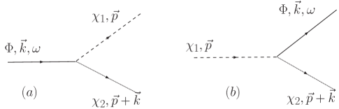
Figure 5: Processes contributing to $\sigma_{0}(k,\omega),\sigma_{a}(k,\omega)$ (a) and to $\sigma_{b}(k,\omega)$ (b). The inverse processes are not shown.

The details of the calculation of the different contributions are relegated to the appendix. The result is summarized as follows:

$$\sigma_{0}(k,\omega)=\frac{g^{2}}{16\pi Q^{2}}\,\text{sign}(\omega)\,\Theta[Q^{2}-(M_{1}+M_{2})^{2}\,]\,\Big{[}(Q^{2})^{2}-2Q^{2}(M^{2}_{1}+M^{2}_{2})+(M^{2}_{1}-M^{2}_{2})^{2}\Big{]}^{\frac{1}{2}}~{}~{};~{}~{}Q^{2}=\omega^{2}-k^{2}$$ (153)

We have explicitly displayed the fact that the zero temperature contribution to the imaginary part is manifestly Lorentz invariant and solely a function of the invariant mass $Q^{2}=\omega^{2}-k^{2}$. The finite temperature contributions are

$$\sigma_{a}(k,\omega;T)=\frac{g^{2}}{16\pi k\,\beta}\,\text{sign}(\omega)\,\Theta[Q^{2}-(M_{1}+M_{2})^{2}\,]\,\Bigg{[}\ln\left(\frac{1-e^{-\beta\omega_{p}^{+}}}{1-e^{-\beta\omega_{p}^{-}}}\right)+M_{1}\leftrightarrow M_{2}\Bigg{]}$$ (154)

$$\sigma_{b}(k,\omega;T)=\frac{g^{2}}{16\pi k\,\beta}\,\text{sign}(\omega)\,\Theta[(M_{1}-M_{2})^{2}-Q^{2}\,]\,\Bigg{[}\ln\left(\frac{1-e^{-\beta|\omega_{p}^{-}|}}{1-e^{-\beta|\omega_{p}^{+}|}}\right)+M_{1}\leftrightarrow M_{2}\Bigg{]}$$ (155)

where

$$\omega_{p}^{\pm}=\frac{|\omega|}{2Q^{2}}(Q^{2}+M^{2}_{1}-M^{2}_{2})\pm\frac{k}{2Q^{2}}\Bigg{[}(Q^{2}+M^{2}_{1}-M^{2}_{2})^{2}-4Q^{2}M_{1}^{2}\Bigg{]}^{\frac{1}{2}}~{}~{};~{}~{}Q^{2}=\omega^{2}-k^{2}.$$ (156)

The real part of the self energy is obtained from the dispersive form (57) and can be separated into a zero temperature and a finite temperature part as follows

$$\mathrm{Re}\widetilde{\Sigma}^{R}(k,\omega;T)=\mathrm{Re}\widetilde{\Sigma}^{R}_{0}(k,\omega)+\mathrm{Re}\widetilde{\Sigma}^{R}_{T}(k,\omega;T)$$ (157)

with

$$\mathrm{Re}\widetilde{\Sigma}^{R}_{0}(k,\omega) = -\frac{1}{\pi}\mathcal{P}\int_{-\infty}^{\infty}\frac{\sigma_{0}(k_{0},k)}{k_{0}-\omega}~{}dk_{0}$$ (158)

$$\mathrm{Re}\widetilde{\Sigma}^{R}_{T}(k,\omega;T) = -\frac{1}{\pi}\mathcal{P}\int_{-\infty}^{\infty}\frac{\sigma_{a}(k_{0},k;T)+\sigma_{b}(k_{0},k;T)}{k_{0}-\omega}~{}dk_{0}$$ (159)

where $\mathcal{P}$ stands for the principal part. We note that both $\sigma_{0}(k,\omega)$ and $\sigma_{a}(k,\omega)$ feature the standard two particle threshold above the light cone at the invariant mass $Q^{2}=(M_{1}+M_{2})^{2}$ whereas the finite temperature contribution $\sigma_{b}(k,\omega)$ has support for invariant mass $Q^{2}\leq(M_{1}-M_{2})^{2}$ even below the light cone and vanishes at $T=0$. In the case of massless particles in the loop this contribution is below the light cone and is identified with Landau dampingkapusta ; brapis ; lebellac . In particular at zero temperature the isolated poles are at $Q^{2}=m^{2}_{P}$, hence if $m^{2}_{P}<(M_{1}-M_{2})^{2}$ the physical particle pole is embedded in the multiparticle continuum and moves off the real axis onto the second (or higher) Riemann sheet in the complex frequency plane. Because of this the physical particle acquires a width. The spectral density for the case $m^{2}_{P}<(M_{1}-M_{2})^{2}$ is depicted in fig. (6)

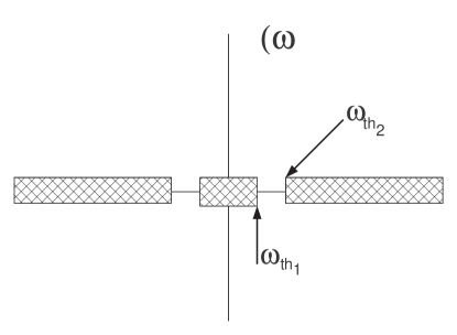
Figure 6: Spectral density $\rho(k,\omega,T)$ for $m^{2}_{P}<(M_{1}-M_{2})^{2}$. The shaded areas are the multiparticle cuts with thresholds $\omega_{th1}=\sqrt{k^{2}+(M_{1}-M_{2})^{2}}$ and $\omega_{th2}=\sqrt{k^{2}+(M_{1}+M_{2})^{2}}$. The single particle poles at $\Omega^{2}_{k}=k^{2}+m^{2}_{P}$ moved off the real axis into an unphysical sheet.

IV.0.1 Zero temperature: $\Omega_{k};Z;\mathcal{C}_{k}$:

Using that $\sigma_{0}(k_{0},k)$ is odd in $k_{0}$ and that it is solely a function of the invariant $P^{2}=k^{2}_{0}-k^{2}$ for $k_{0}>0$, it is straightforward to find the following manifestly Lorentz invariant result

$$\mathrm{Re}\widetilde{\Sigma}^{R}_{0}(k,\omega)=-\frac{1}{\pi}\mathcal{P}\int_{(M_{1}+M_{2})^{2}}^{\infty}\frac{\sigma_{0}(P^{2})}{P^{2}-Q^{2}}~{}dP^{2}~{}~{};~{}~{}Q^{2}=\omega^{2}-k^{2}$$ (160)

where we have explicitly exhibited the two particle threshold in the lower limit. Lorentz invariance requires that the single particle pole features the dispersion relation $\Omega^{2}_{k}=k^{2}+m^{2}_{P}$, and so the equation that determines the single particle physical poles, namely eqn. (117) is given by

$$m^{2}_{P}-m^{2}-\mathrm{Re}\widetilde{\Sigma}^{R}_{0}(Q^{2}=m^{2}_{P})=0$$ (161)

From the results of the previous section (see eqn. (129)) the wave function renormalization constant is given by

$$Z^{-1}=1+\frac{1}{\pi}\mathcal{P}\int_{(M_{1}+M_{2})^{2}}^{\infty}~{}\frac{\sigma_{0}(P^{2})}{(P^{2}-m^{2}_{P})^{2}}~{}dP^{2}\,,$$ (162)

Separating the residue at the physical particle pole and following the steps described in section (III.2) the renormalized spectral density (135,136) at zero temperature can now be written in the following simple form

$$\rho_{r}(k,\omega;T=0)=\frac{1}{\pi}\,\frac{\left[\sigma_{0,r}(Q^{2})+2\omega\epsilon\right]}{\left[(Q^{2}-m^{2}_{P})\Big{(}1-\Pi_{0,r}(Q^{2})\Big{)}\right]^{2}+\left[\sigma_{0,r}(Q^{2})+2\omega\epsilon\right]^{2}}=\mathrm{sign}(\omega)\,\delta(\omega^{2}-\Omega^{2}_{k})+\rho_{c,r}(k,\omega;T=0)$$ (163)

where $\sigma_{0,r}(k,\omega)=Z\sigma_{0}(k,\omega)$ is given by the expression (153) but with the coupling constant replaced by the renormalized coupling $Zg^{2}=g^{2}_{r}$

The continuum contribution is given by

$$\rho_{c,r}(k,\omega;T=0)=\frac{1}{\pi}\,\frac{\sigma_{0,r}(Q^{2})}{\left[(Q^{2}-m^{2}_{P})\Big{(}1-\Pi_{0,r}(Q^{2})\Big{)}\right]^{2}+\Big{[}\sigma_{0,r}(Q^{2})\Big{]}^{2}}\;,$$ (164)

with

$$\Pi_{0,r}(Q^{2})=-\frac{1}{\pi}(Q^{2}-m^{2}_{P})~{}\mathcal{P}\int_{(M_{1}+M_{2})^{2}}^{\infty}\frac{\sigma_{0,r}(P^{2})}{(P^{2}-Q^{2})(P^{2}-m^{2}_{P})^{2}}~{}dP^{2}$$ (165)

where we have made explicit the two particle threshold in the lower limit of the integral.

The exact expression for $Z$ given by the sum rule (119) coincides with $Z$ given by eqn. (162) to lowest order in perturbation theory ($\mathcal{O}(g^{2})$).

Up to $\mathcal{O}(g^{2})$ we can neglect $\sigma_{0}(k,\omega)$ as well as $\Pi_{0,r}(k,\omega)$ in the denominator of the continuum contribution (164) because $Q^{2}\geq(M^{2}_{1}+M^{2}_{2})>m^{2}_{P}$ and the denominator is never perturbatively small. Therefore to leading order in the coupling we can approximate

$$\rho_{c,r}(k,\omega;T=0)\simeq\frac{1}{\pi}\,\frac{\sigma_{0,r}(Q^{2})}{(Q^{2}-m^{2}_{P})^{2}}\;.$$ (166)

The renormalized spectral function at finite temperature can be separated into the contributions from the different multiparticle cuts,

$$\rho_{r}(k,\omega,T)=\rho_{I,r}(k,\omega,T)+\rho_{II,r}(k,\omega,T)$$ (167)

where the contribution with support above the two particle cut is

$$\rho_{I,r}(k,\omega;T)=\frac{1}{\pi}\,\frac{\left[\sigma_{0,r}(k,\omega)+\sigma_{a,r}(k,\omega;T)\right]}{\left[(Q^{2}-m^{2}_{P})\Big{(}1-\Pi_{0,r}(Q^{2})\Big{)}-\mathrm{Re}\widetilde{\Sigma}^{R}_{T,r}(k,\omega;T)\right]^{2}+\Big{[}\sigma_{0,r}(Q^{2})+\sigma_{a,r}(k,\omega;T)\Big{]}^{2}}$$ (168)

and that which has support below the light cone given by

$$\rho_{II,r}(k,\omega;T)=\frac{1}{\pi}\,\frac{\sigma_{b}(k,\omega;T)}{\left[(Q^{2}-m^{2}_{P})\Big{(}1-\Pi_{0,r}(Q^{2})\Big{)}-\mathrm{Re}\widetilde{\Sigma}^{R}_{T,r}(k,\omega;T)\right]^{2}+\Big{[}\sigma_{b,r}(k,\omega;T)\Big{]}^{2}}$$ (169)

where again the renormalized quantities are obtained from the unrenormalized ones by replacing $g\rightarrow g_{r}=Zg$.

Since $\rho_{I,r}(k,\omega)$ has support only for $|\omega|>\sqrt{k^{2}+(M^{2}_{1}+M^{2}_{2})}$ its denominator is never perturbatively small, therefore to leading order $\mathcal{O}(g^{2})$ in the perturbative expansion it can be approximated by

$$\rho_{I,r}(k,\omega;T)\simeq\frac{1}{\pi}\,\frac{\left[\sigma_{0,r}(k,\omega)+\sigma_{a,r}(k,\omega;T)\right]}{(\omega^{2}-k^{2}-m^{2}_{P})^{2}}$$ (170)

For $\rho_{II,r}(k,\omega)$ we must keep the full expression because for $m^{2}_{P}<(M_{1}-M_{2})^{2}$ the denominator becomes perturbatively small for $\omega^{2}\sim k^{2}+m^{2}_{P}$. Therefore the final expression for the asymptotic distribution function (138) to leading order in the coupling ($\mathcal{O}(g^{2})$) is given by

$$\mathcal{N}(k,T)=\mathcal{N}_{I}(k;T)+\mathcal{N}_{II}(k,T)$$ (171)

where the different contributions reflect the different multiparticle cuts, namely

$$\mathcal{N}_{II}(k,T) = \int_{0}^{\infty}\Bigg{(}\frac{\omega^{2}+\Omega^{2}_{k}}{2\,\Omega_{k}}\Bigg{)}\Bigg{\{}\left[1+2n(\omega)\right]\rho_{II,r}(k,\omega,T)\Bigg{\}}\,{d\omega}\,-\frac{1}{2}$$ (172)

$$\mathcal{N}_{I}(k,T) = \frac{2}{\pi}\int_{\omega_{th}(k)}^{\infty}\Bigg{[}\frac{\omega^{2}+\Omega^{2}_{k}}{2\,\Omega_{k}(\omega^{2}-\Omega^{2}_{k})^{2}}\Bigg{]}\Bigg{\{}n(\omega)\Big{[}\sigma_{0,r}(k,\omega)+\sigma_{a,r}(k,\omega;T)\Big{]}+\frac{1}{2}\sigma_{a,r}(k,\omega;T)\Bigg{\}}\,{d\omega}\,,$$ (173)

where $\omega_{th}(k)=\left[k^{2}+(M_{1}+M_{2})^{2}\right]^{\frac{1}{2}}$ is the two particle cut.

IV.1 The approach to equilibrium:

Before we study the asymptotic distribution function we address the approach to equilibrium. The time evolution of the (interpolating) number operator $N_{k}(t)$ given by eqns. (89-91) is completely determined by the real time evolution of the solution $f_{k}(t)$ given by eqn. (76). For $m_{P}<|M_{1}-M_{2}|$ the particle acquires a width through the two body decay of the heavier particle in the bath and the particle pole is now embedded in the continuum for $Q^{2}<(M_{1}-M_{2})^{2}$, which is the relevant part of the spectral density is $\sigma_{b}(k,\omega,T)$ given in eqn. (155). In the Breit Wigner approximation, the spectral density is given by eqns. (93,92,94) with

$$\Gamma_{k}(T)=\mathcal{Z}_{k}\,\frac{\sigma_{b}(k,\mathcal{W}_{k}(T),T)}{2\,\mathcal{W}_{k}(T)}$$ (174)

The real time evolution of the solution $f_{k}(t)$ in the Breit-Wigner approximation is given by eqn. (99). Figure (7) displays both the exact solution (76) and the Breit-Wigner approximation (99) for $k=0$. The exact and approximate solutions are indistinguishable during the time scale of the numerical evolution as gleaned from this figure.

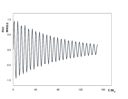
Figure 7: The functions $f_{k=0}(t)$ and $f^{BW}_{k=0}(t)$ vs $t\,m_{P}$ for $g^{2}/(16\pi^{2}m^{2}_{P})=0.01$ $M_{1}=4m_{P}\,;\,M_{2}=m_{P}\,;\,T=10m_{P}$. For these values of the parameters we find numerically: $\mathcal{Z}_{0}(T)=0.998\;,\;\mathcal{W}_{0}(T)=0.973m_{P}\;,\;\Gamma_{0}(T)=0.012m_{P}$. The exact solution and the Breit-Wigner approximation are indistinguishable.

The asymptotic long time evolution is determined by the behavior of the spectral density near the thresholds and is typically of the form of a power lawthreshold . However, such asymptotic behavior sets in at very long times, beyond the regime in which our numerical study is trustworthy. It is numerically exceedingly difficult to extract the exponential relaxation from the power laws that dominate at asymptotically long time because the amplitude becomes very small in the weak coupling case.

The main conclusion is that the distribution function approaches thermalization and becomes insensitive to the initial conditions for time scales $t>\tau_{k}=1/2\Gamma_{k}(T)$, where $\Gamma_{k}(T)$ is the quasiparticle relaxation rate.

IV.2 The asymptotic distribution function:

In the Breit-Wigner approximation and assuming a very narrow resonance near the physical particle pole

$$\rho_{II,r}(k,\omega,T)\sim\frac{1}{\pi}\,\frac{\mathrm{sign}(\omega)\,\Gamma_{k}}{(\omega^{2}-\Omega^{2}_{k})^{2}+\Gamma^{2}_{k}}\sim\mathrm{sign}(\omega)\delta(\omega^{2}-\Omega^{2}_{k})$$ (175)

where in the second term on the right hand side the width has been neglected by assuming a very narrow resonance at $\Omega_{k}$. Therefore in this narrow width approximation one would expect that the different contributions are given by

$$\mathcal{N}_{II}(k,T)\sim n(\Omega_{k})~{}~{};~{}~{}\mathcal{N}_{I}(k,T)=\mathcal{O}(g^{2})$$ (176)

where $n(\Omega_{k})$ is the Boltzmann distribution function for the stable particle. This rather simple analysis would lead to the conclusion that the corrections to the equilibrium abundance are perturbatively small.

However, even for weakly coupled theories we expect this simple argument to be incorrect both in the high and low temperature regimes. The main reason for this expectation is that the approximation (175) suggests that this argument neglects the fact that the spectral density has support for frequencies smaller than the position of the physical particle pole (namely for $|\omega|\neq\Omega_{k}$). From the expression (172) it is clear that the region of small $\omega$ will lead to a substantial correction since for $\omega\ll T$ the Bose-Einstein distribution function in (172) becomes $n(\omega)\sim T/\omega>>1$, thus the region of $|\omega|<\Omega_{k}$ and in particular $|\omega|\ll T$ gives a non-trivial contribution to the abundance. The region of spectral density for $|\omega|>\Omega_{k}$ will yield a much smaller, but non-negligible contribution. Furthermore in the high temperature limit $T\gg k,m_{P},M_{1,2}$ the width is expected to become large. This can be gleaned from the expression for $\sigma_{b}(\omega,k,T)$ in eqn. (152), which for $T\gg\omega^{1,2}_{p}$ is proportional to $T$. This is clearly a statement that at high temperatures there is a large population of heavy particles which results in a larger number of processes $\chi_{1}\leftrightarrow\Phi\,\chi_{2}$ in the medium, thereby increasing the width of the particle $\Phi$. As the width of the spectral density near the physical particle pole increases, the spectral density has larger support in the small $\omega$ region, thereby increasing the off-shell contributions to the abundance. These arguments will be confirmed both analytically and numerically below.

We now study numerically and analytically the asymptotic distribution function to assess precisely the magnitude and origin of the corrections to the equilibrium abundance. The parameter space is fairly large, thus we consider separately the cases of small momenta $k\ll m_{P},M_{1},M_{2},T$ and the case of large momenta $k\gg m_{P},M_{1},M_{2},T$ choosing the unit of energy to be the zero temperature pole mass of the particle, $m_{P}$ and keeping the value of the masses of the heavy fields fixed with $M_{1}>M_{2}+m_{P}$.

IV.2.1 $k=0$

The limit $k=0$ of the spectral density can be easily obtained from the expressions given above (153-155). Of particular importance is the high temperature limit of $\sigma_{b}(0,\omega,T)$ since this contribution to the spectral density determines the width of the spectral function near the physical particle pole $\Gamma_{0}(T)$ given by eqn. (174).

A straightforward calculation leads to the following result in the limit $T\gg m_{P}\,,\,M_{1,2}$,

$$\frac{\sigma_{b}(0,m_{P},T)}{2\,m_{P}}=\frac{g^{2}T}{8\pi^{2}}\,\frac{\Big{[}m^{4}_{P}+(M^{2}_{1}-M^{2}_{2})^{2}-2m^{2}_{P}(M^{2}_{1}+M^{2}_{2})\Big{]}^{\frac{1}{2}}}{\Big{[}(M^{2}_{1}-M^{2}_{2})^{2}-m^{4}_{P}\Big{]}}$$ (177)

Figure 8: The spectral density $\rho_{II}(k=0,\omega,T)$ vs $\omega/m_{P}$ for $g^{2}/(16\pi^{2}m^{2}_{P})=0.01$ $M_{1}=4m_{P}\,;\,M_{2}=m_{P}$ and $T/m_{p}=10,30,100$ respectively.

We note that this expression for the width is classical since restoring $g^{2}\rightarrow g^{2}\hbar\,;\,T\rightarrow T/\hbar$ the expression above is independent of $\hbar$. This is a consequence of the fact that the high temperature limit is completely determined by the Rayleigh-Jeans part of the Bose-Einstein distribution function. As a result when the temperature is much larger than all mass scales, the width is proportional to $T$ and the spectral density becomes wider, enhancing the off-shell contributions. Fig. (8) displays the spectral density for several values of the temperature highlighting the broadening for large temperature. It is clear from this figure that at very high temperatures perturbation theory breaks down in this model since the width can become comparable to the physical mass or the position of the pole. This situation has been previously noticed in a scalar field theory at high temperatures, and a finite temperature renormalization group was introduced to provide a non-perturbative resummationhotRG .

Restricting ourselves to the regime in temperature within which perturbation theory is still reliable, namely for $\Gamma_{0}(T)\ll m_{P}$, we study the departure of the distribution function from the Bose-Einstein form (for $k=0$) numerically.

Figure (9) displays the quantity

$$\Delta(T)=\frac{\mathcal{N}(k=0,T)-n(m_{P})}{n(m_{P})}$$ (178)

for a weakly coupled case in the range of temperatures $1\leq T/m_{p}\leq 20$ for $M_{1}=4m_{P}\,,\,M_{2}=m_{P}$ within which we find numerically that $\Gamma_{0}(T)/m_{P}\leq 0.1$ which we use as a reasonable criterion for the validity of perturbation theory (see fig. 8).

Figure 9: The ratio $\Delta(T)=(\mathcal{N}(0,T)-n(m_{P}))/n(m_{P})$ vs $m_{P}/T$ for $g^{2}/(16\pi^{2}m^{2}_{P})=0.01$ $M_{1}=4m_{P}\,;\,M_{2}=m_{P}$.

This figure clearly indicates that even within the high temperature regime where perturbation theory is reliable and the spectral density still features a rather narrow Breit-Wigner peak, there are substantial departures from the Bose-Einstein form in the equilibrium distribution function. At low temperatures fig. (9) clearly displays an exponential suppression and the distribution function essentially becomes the Bose-Einstein distribution. In this limit the width is extremely small and the spectral density is almost a delta function on the physical particle mass shell, and the off-shell effects are perturbatively small.

IV.2.2 $k\gg T,m_{P},M_{1,2}$

In the limit of large momenta several interesting features emerge: i) the width of the spectral density becomes very small, this is a consequence of the fact that there are very few heavy states for large momenta in the heat bath if the momentum is large. The width as a function of $k$ is depicted in fig. (10), which displays clearly this behavior. ii) As a function of the variable $\omega$, the position of the peak in the spectral density becomes closer to the threshold for $k\gg m_{P},M_{1,2}$. As a result of both these effects the spectral distribution becomes strongly peaked near threshold and the threshold moves to larger values of the frequency, thus leaving behind a larger region of the spectra off-shell for frequencies smaller than the position of the peak. The spectral density while small away from the peak is, however, non-vanishing and the fact that there is now a larger region in frequency $\omega$ below the (narrow) peak, brings about a competition of scales as can be understood from the following argument. The very narrow peak (almost a delta function at $\omega=\Omega_{k}\sim k$) leads to a contribution $\mathcal{N}_{II}(k,T)\sim n(\Omega_{k})$, which for $k\gg T$ is $\ll 1$. This on-shell contribution competes against the off-shell contributions from integrating the spectral density for $\omega<\Omega_{k}$ which is also very small because $\sigma_{b}(k,\omega,T)/\Omega^{2}_{k}\ll 1$ but for $\omega\ll T$ is multiplied by the Bose enhancement factor $\sim T/\omega$. The competition between the “on-shell” contribution $n(\Omega_{k})$ and the off-shell contributions is studied numerically.

Figure 10: The width $\Gamma(k,T)$ in units of $m_{P}$ vs $k/m_{P}$ for $k\gg T$ for $T=m_{P}$ for $g^{2}/(16\pi^{2}m^{2}_{P})=0.01$ $M_{1}=4m_{P}\,;\,M_{2}=m_{P}$.

Fig. (11) displays both the Bose-Einstein distribution function $n(\Omega_{k})$ and the asymptotic distribution function $\mathcal{N}(k,T)$ in the limit $k\gg T,m_{P},M_{1,2}$.

Figure 11: The distribution functions $\mathcal{N}(k,T)$ given by eqn. (171) (solid line) vs. the Bose-Einstein distribution $N_{BE}(k,T)$ (dashed line) as a function of $k/m_{P}$ for $T=m_{P}$; $g^{2}/(16\pi^{2}m^{2}_{P})=0.01$; $M_{1}=4m_{P}\,;\,M_{2}=m_{P}$.

It is clear from this figure that while the distribution function $\mathcal{N}(k,T)$ is strongly suppressed for $k\gg T$ it is larger than the Bose-Einstein distribution. The main reason for this enhancement is precisely the competition mentioned above, namely the position of the peak in the spectral density moves towards threshold which for large $k$ corresponds to large values of the frequency $\omega$. Therefore there is a large region in which the spectral density is very small but non-vanishing for $\omega<\Omega_{k}$. Clearly the part of the spectral density with support for $\omega>\Omega_{k}$ yields a much smaller contribution to the distribution function. Furthermore, for $\omega\ll T$ the factor $n(\omega)\sim T/\omega\gg 1$ which enhances further the off-shell contributions.

These results in the different regimes can be summarized as follows:

• In the high temperature regime the larger abundance of heavier particles in the bath leads to a broadening of the spectral density. This broadening in turn results in a larger off-shell contribution to the abundance $\mathcal{N}(k,T)$ and an enhancement of the distribution function over the Bose-Einstein result. The off-shell region of small frequency yields a substantial contribution because of the factor $n(\omega)\sim T/\omega$ in (138). In the model considered perturbation theory breaks down at high temperature and the imaginary part on-shell becomes classical. This situation is akin to the case of a self-interacting bosonic field theory studied in ref. hotRG . A high temperature renormalization group resummation program such as in ref.hotRG may be required to provide a non-perturbative resummation.

• For momenta much larger than the mass scales and the temperature there is also a large enhancement of the distribution function $\mathcal{N}(k,T)$ over the Bose-Einstein result. In this case the spectral density features a very narrow resonance near the position of the physical pole at $\omega\simeq\Omega_{k}$, which however moves closer to threshold. For large $k$ the off-shell region of support of the spectral density becomes larger and though the spectral density is strongly suppressed, the off-shell contribution from the region $\omega<\Omega_{k}$ competes with the contribution from the on-shell pole, namely the Bose-Einstein distribution function $n(\Omega_{k})$ because for $k>>T$ $n(\Omega_{k})\ll 1$. The off-shell contribution from the region $\omega<<\Omega_{k}$ is comparable to or larger than $n(\Omega_{k})$ for $k\gg T$ and is enhanced in the region $\omega\ll T$ by the factor $n(\omega)\sim T/\omega$.

While these results may be particular to the model studied, we expect most of these features to be robust and fairly general. In particular at high temperature it is physically reasonable to expect a thermal broadening of the spectral density either from collisions, many-body decays or Landau damping as in the case studied here. Broadening of the spectral function yields a larger contribution from the small $\omega$ region which is enhanced further by the factor $n(\omega)\sim T/\omega$ for $\omega\ll T$. Therefore a substantial departure of the distribution function $\mathcal{N}(k,T)$ from the Bose-Einstein distribution is expected at high temperature. A possible breakdown of perturbation theory in the high temperature regime may require the implementation of a non-perturbative resummation procedure akin to that introduced in ref.hotRG . At low temperatures, much lower than the mass and momentum scales a departure from simple Bose-Einstein is also expected. In this case even though the spectral function features a sharp and narrow peak at a position very near the physical particle pole, the Bose-Einstein distribution function is very small. Hence the off-shell region $\omega<<\Omega_{k}$ of the spectral function will lead to a substantial contribution which is further enhanced by the factor $n(\omega)\sim T/\omega$ for $\omega\ll T$. Again because the temperature is much smaller than any of the scales, the spectral density will be exponentially suppressed off shell and the equilibrium abundance will reflect this suppression, but just as in the case studied here, may still be larger than the simple Bose-Einstein abundance. Of course our study within this particular model serves only as a guidance and the details of the enhancement will depend on the theory under consideration, but the main lesson learned here is that the off-shell, small frequency region of the spectral density yields a substantial contribution to the equilibrium abundance in interacting theories.

V Boltzmann kinetics in renormalized perturbation theory

It is important to understand the origin of the differences between the quantum kinetic equation for the distribution function (89) and the usual quantum Boltzmann equation. Therefore in this section we provide a derivation of the quantum Boltzmann equation in renormalized perturbation theory to highlight the origin of the different equilibrium abundances. We assume that the bath is in equilibrium just as we did in our derivation of the effective action and the time evolution for the distribution function in the previous sections.

The quantum Boltzmann equation is a differential equation for the single particle distribution function. However, as we have discussed in detail above, the physical particles have mass $m_{P}$ and the Heisenberg field operators create physical particles out of the vacuum with an amplitude determined by the wave function renormalization. Therefore in order to account for the mass and wave function renormalization, and to obtain the kinetic Boltzmann equation for the physical particles it is convenient to re-write the Lagrangian by introducing counterterms, namely

$$\mathcal{L}= \frac{1}{2}\partial_{\mu}\Phi_{r}\partial^{\mu}\Phi_{r}-\frac{1}{2}m^{2}_{P}\Phi^{2}_{r}+\sum_{i=1}^{2}\Bigg{[}\frac{1}{2}\partial_{\mu}\chi_{i}\partial^{\mu}\chi_{i}-\frac{1}{2}M^{2}_{i}\chi^{2}_{i}\Bigg{]}-g_{r}\Phi_{r}\,\chi_{1}\,\chi_{2}+\mathcal{L}_{count}+\mathcal{L}_{int}[\chi_{1}\,;\,\chi_{2}]$$ (179)

$$\mathcal{L}_{count}= \frac{1}{2}(Z-1)\partial_{\mu}\Phi_{r}\partial^{\mu}\Phi_{r}-\frac{1}{2}\Delta m^{2}\Phi^{2}_{r}$$ (180)

where $g_{r}=\sqrt{Z}g$ and we assume that the renormalization aspects of the fields $\chi_{1,2}$ had already been included in $\mathcal{L}_{int}[\chi_{1}\,;\,\chi_{2}]$ . The counterterms in (180) are treated systematically in perturbation theory along with the cubic interaction. Note that $Z-1\,,\,\Delta m^{2}$ are both of $\mathcal{O}(g^{2})$.

The renormalized field $\Phi_{r}$ is expanded in terms of creation and annihilation operators of physical Fock states,

$$\Phi_{r}(\vec{x},t) = \frac{1}{\sqrt{V}}\sum_{\vec{k}}\Phi_{\vec{k}}(t)e^{i\vec{k}\cdot\vec{x}}$$ (181)

$$\Phi_{\vec{k}}(t) = \frac{1}{\sqrt{2\Omega_{k}}}\left[a_{\vec{k}}\,e^{-i\Omega_{k}\,t}+a^{\dagger}_{-\vec{k}}\,e^{i\Omega_{k}\,t}\right]$$ (182)

and a similar expansion for the bath fields $\chi_{1},\chi_{2}$ in terms of creation and annihilation operators and the corresponding frequencies $\omega_{k}^{(1,2)}$. The total interaction Lagrangian is

$$L_{int}=\frac{g_{r}}{\sqrt{V}}\sum_{\vec{k}}\sum_{\vec{p}}\Phi_{k}\,\chi_{1,\vec{p}}\,\chi_{2,-\vec{p}-\vec{k}}+L_{count}$$ (183)

where $L_{count}$ is the counterterm Lagrangian. The kinetic Boltzmann equation for the occupation number of the Fock quanta of the field $\Phi$ is

$$\frac{dN_{k}}{dt}=\frac{dN_{k}}{dt}\Bigg{|}_{gain}-\frac{dN_{k}}{dt}\Bigg{|}_{loss}$$ (184)

The gain and loss terms are obtained by calculating the transition probabilities per unit time for processes that lead to the increase (gain) and decrease (loss) the occupation number, namely $dN_{k}(t)/dt=dP_{k}/dt$. Within the framework of the kinetic description such calculation is carried out by implementing Fermi’s Golden rule. The processes that lead to the increase or decrease of the population are read-off the interaction and energy conservation emerges as a consequence of taking the long time limit as is manifest in Fermi’s Golden rule. The cubic interaction term in $L_{int}$ gives rise to several different processes which are gleaned by expanding the product in terms of the creation and annihilation operators of all the fields involved. The different phases that enter in such terms determine the energy conservation delta functions in Fermi’s Golden rule. Some of the processes are depicted in fig. (5). When $m_{P}<M_{1},M_{2}$ the quanta of the field $\Phi$ cannot decay into those of the bath fields, however if $M_{1}>M_{2}+m_{P}$ (or $M_{2}>M_{1}+m_{P}$) the heavier bath field can decay into particles of $\Phi$ therefore increasing the population. This process is depicted in fig. (5-(b)). The inverse process contributes to the loss term. Let us consider the case $M_{1}>M_{2}+m_{P}$ (the case $M_{2}>M_{1}+m_{P}$ is similar by $M_{2}\leftrightarrow M_{1}$). The only process that leads to the gain in the population by energy conservation is $\chi_{1}\rightarrow\Phi\,\chi_{2}$ and consequently the only process that leads to the loss of population with energy conservation is the inverse process of annihilation $\Phi\,\chi_{2}\rightarrow\chi_{1}$. The calculation of the gain and loss terms is as follows: consider the initial Fock state $|N_{\vec{k}},n^{(1)}_{\vec{p}},n^{(2)}_{\vec{p}+\vec{k}}\rangle$ where $N$ is the occupation of particles of $\Phi$ and $n^{(1,2)}$ that for the respective bath fields. To lowest order in the coupling $g$ the interaction from the counterterm Lagrangian does not contribute to the gain or loss, but only to forward scattering since these terms are already of $\mathcal{O}(g^{2})$ and the transition probabilities will be at least of $\mathcal{(}g^{3})$. Thus to lowest order $\mathcal{O}(g^{2})$, the gain term arises from the following matrix element

$$\mathcal{M}_{gain}=-\frac{ig_{r}}{\sqrt{V}}\langle N_{\vec{k}}+1,n^{(1)}_{\vec{p}}-1,n^{(2)}_{\vec{p}+\vec{k}}+1\Big{|}\int_{-\infty}^{\infty}dt\,\Phi_{k}(t)\,\chi_{1,\vec{p}}(t)\,\chi_{2,-\vec{p}-\vec{k}}(t)\Big{|}N_{\vec{k}},n^{(1)}_{\vec{p}},n^{(2)}_{\vec{p}+\vec{k}}\rangle$$ (185)

The limits in the time integral had been extended to $\pm\infty$ according to Fermi’s Golden rule which leads to energy conservation. The calculation of this matrix element is straightforward, taking the absolute value squared of this matrix element, summing over $\vec{p}$ and averaging over the occupation numbers of the particles in the bath, which is assumed in equilibrium, one obtains the inclusive transition probability

$$P_{gain}=\frac{2\,t}{2\Omega_{k}}\frac{g^{2}}{32\pi^{2}}\Big{(}1+N_{k}\Big{)}\int\frac{d^{3}\vec{p}}{\omega_{\vec{p}}^{(1)}\omega_{\vec{p}+\vec{k}}^{(2)}}\,n(\omega_{\vec{p}}^{(1)})\,\Big{[}1+n(\omega_{\vec{p}+\vec{k}}^{(2)})\Big{]}\,\delta\left(\Omega_{k}+\omega_{\vec{p}+\vec{k}}^{(2)}-\omega_{\vec{p}}^{(1)}\right)$$ (186)

where $n(\omega_{\vec{p}}^{(1,2)})$ are the Bose-Einstein distribution functions since the thermal bath is assumed to remain in equilibrium. To obtain the above expression we have used $\Big{|}2\pi\delta\left(\Omega_{k}+\omega_{\vec{p}+\vec{k}}^{(2)}-\omega_{\vec{p}}^{(1)}\right)\Big{|}^{2}=2\pi\delta\left(\Omega_{k}+\omega_{\vec{p}+\vec{k}}^{(2)}-\omega_{\vec{p}}^{(1)}\right)t$ where $t$ is the total interaction time. A similar calculation leads to the total transition probability for the loss process:

$$P_{loss}=\frac{2\,t}{2\Omega_{k}}\frac{g^{2}}{32\pi^{2}}N_{k}\int\frac{d^{3}\vec{p}}{\omega_{\vec{p}}^{(1)}\omega_{\vec{p}+\vec{k}}^{(2)}}\,\Big{[}1+n(\omega_{\vec{p}}^{(1)})\Big{]}\,n(\omega_{\vec{p}+\vec{k}}^{(2)})\,\delta\left(\Omega_{k}+\omega_{\vec{p}+\vec{k}}^{(2)}-\omega_{\vec{p}}^{(1)}\right)$$ (187)

The kinetic equation can now be written in the following form

$$\frac{dN_{k}}{dt}=(1+N_{k})\,\gamma^{>}_{k}-N_{k}\,\gamma^{<}_{k}$$ (188)

The gain and loss rates are given by

$$\gamma^{>}_{k} = \frac{2}{2\Omega_{k}}\frac{g^{2}}{32\pi^{2}}\int\frac{d^{3}\vec{p}}{\omega_{\vec{p}}^{(1)}\omega_{\vec{p}+\vec{k}}^{(2)}}\,n(\omega_{\vec{p}}^{(1)})\,\Big{[}1+n(\omega_{\vec{p}+\vec{k}}^{(2)})\Big{]}\,\delta\left(\Omega_{k}+\omega_{\vec{p}+\vec{k}}^{(2)}-\omega_{\vec{p}}^{(1)}\right)$$ (189)

$$\gamma^{<}_{k} = \frac{2}{2\Omega_{k}}\frac{g^{2}}{32\pi^{2}}\int\frac{d^{3}\vec{p}}{\omega_{\vec{p}}^{(1)}\omega_{\vec{p}+\vec{k}}^{(2)}}\,\Big{[}1+n(\omega_{\vec{p}}^{(1)})\Big{]}\,n(\omega_{\vec{p}+\vec{k}}^{(2)})\,\delta\left(\Omega_{k}+\omega_{\vec{p}+\vec{k}}^{(2)}-\omega_{\vec{p}}^{(1)}\right)$$ (190)

Since the bath particles are in thermal equilibrium with a Bose-Einstein distribution function the detailed balance condition follows, namely

$$\gamma^{>}_{k}=e^{-\beta\,\Omega_{k}}\,\gamma^{<}_{k}$$ (191)

The solution of the Boltzmann kinetic equation (188) is the following

$$N_{k}(t)=n(\Omega_{k})+[N_{k}(0)-n(\Omega_{k})]e^{-\gamma_{k}\,t}$$ (192)

where

$$\gamma_{k}=\gamma^{<}_{k}\,-\,\gamma^{>}_{k}=\frac{2}{2\Omega_{k}}\,\frac{g^{2}}{32\pi^{2}}\,\int\frac{d^{3}\vec{p}}{\omega_{\vec{p}}^{(1)}\omega_{\vec{p}+\vec{k}}^{(2)}}\,\Big{[}n(\omega_{\vec{p}+\vec{k}}^{(2)})-n(\omega_{\vec{p}}^{(1)})\Big{]}\delta\left(\Omega_{k}-\omega_{\vec{p}}^{(1)}+\omega_{\vec{p}+\vec{k}}^{(2)}\right)$$ (193)

Comparing this expression with those for the imaginary part of the self energy given by (149,150,151,152) it is straightforward to see that

$$\gamma_{k}=2\,\frac{\mathrm{Im}\tilde{\Sigma}^{R}_{r}(k,\Omega_{k},T)}{2\Omega_{k}}$$ (194)

where

$$\mathrm{Im}\tilde{\Sigma}^{R}_{r}(k,\Omega_{k},T)=\sigma_{b,r}(k,\Omega_{k},T)$$ (195)

This expression for the relaxation rate should be compared to the decay rate for the single quasiparticle $\Gamma_{k}$ given by eqn. (95,99)). Since the quasiparticle residue in perturbation theory is $\mathcal{Z}_{k}(T)=1+\mathcal{O}(g^{2})$ and the difference between the quasiparticle frequency $\mathcal{W}_{k}(T)$ and the single particle frequency $\Omega_{k}$ is of $\mathcal{O}(g^{2})$ to leading order in the coupling $g$, the relaxation rate of the distribution function $\gamma_{k}$ and that of the single quasiparticle $\Gamma_{k}$ (see eqn. (95)) is

$$\gamma_{k}=2\Gamma_{k}+\mathcal{O}(g^{4})$$ (196)

We have provided this derivation of the usual quantum Boltzmann equation and its solution in the case when the bath remains in equilibrium to highlight the similarities and differences with the real time evolution of the distribution function given by eqn. (89):

• The derivation above clearly shows that the Fock states that enter in the matrix elements (185) are the asymptotic free field Fock states associated with physical particles of mass $m_{P}$. This is similar to the definition of the interpolating number operator (81) which is based on the free field asymptotic physical states, and includes both mass and wave-function renormalization.

• By implementing Fermi’s golden rule, namely taking the time interval to infinity, thereby enforcing the on shell delta function, extracting the linear time dependence and dividing by time to provide a local differential equation for the time evolution of the distribution function all memory aspects have been neglected. Namely implementing Fermi’s golden rule results in neglecting memory effects, which in turn results in only on-shell processes contributing to the rate equation. Contrary to this, the real time evolution of the distribution function (89) includes memory effects as is manifest in the time integrals (90,91) in (89). In turn these time integrals keep memory of the past time evolution, and at asymptotically long time lead to the full spectral density as manifest in eqn. (102), not just an on-shell delta function. The presence of the full spectral density in the asymptotic distribution includes the off-shell contributions discussed in the previous section. This discussion brings to the fore that one of the main origins of the differences can be traced to memory effects and the fact that the real time evolution of the distribution function (89) is non-Markovian. The memory of the past time evolution translates in off-shell processes through the full spectral density.

• As emphasized in section (II) the expression (89) for the quantum kinetic distribution function implies a Dyson-like resummation of the perturbative expansion and includes consistently the renormalization aspects associated with asymptotic single particle states, namely the correct pole mass and the wave function renormalization. The dependence of the asymptotic distribution function on the full spectral density is a consequence of the fluctuation-dissipation relation.

VI Conclusions and discussion

Motivated by a critical reassessment of the applicability of Boltzmann kinetics in the early Universe, in this article we studied the abundance of physical quanta of a field $\Phi$ in a thermal plasma by introducing a quantum kinetic description based on the non-equilibrium effective action for this field. We focused on understanding the equilibrium abundance of particles that are stable in the vacuum and interact with heavier particles which constitute a thermal bath.

The non-equilibrium effective action is obtained by integrating out the heavy particles to lowest order in the coupling of the field $\Phi$ to the bath but in principle to all orders in the coupling of the heavy fields amongst them. We show that the non-equilibrium effective action leads to a Langevin stochastic description with a Gaussian but colored noise and a non-Markovian self-energy kernel. The correlation function of the noise and the non-Markovian self-energy kernel are related by a generalized fluctuation dissipation relation. The correlation functions are determined by the solution of this Langevin equation which furnishes a Dyson resummation of the perturbative expansion. We introduced a definition of the single physical particle distribution function in terms of a fully renormalized interpolating Heisenberg number operator based on asymptotic theory. The real time evolution of this single particle distribution function is completely determined by the solution of the Langevin equation.

We show that in a heat bath at finite temperature this number operator becomes insensitive to the initial conditions after a time scale $\approx 1/2\,\Gamma_{k}(T)$, where $\Gamma_{k}(T)$ is the single quasiparticle relaxation rate. We prove that the asymptotic long time limit of this distribution function describes full thermalization of the $\Phi$ particle with the thermal bath. The equilibrium distribution function depends on the full spectral density and includes off-shell corrections as a result of the non-Markovian real time evolution (with memory) and the fluctuation-dissipation relation. Its expression is given by eqn. (138). We argue that while we obtained the distribution function in the case of a field linearly coupled to a thermal bath of heavier particles, the final form of the distribution function at asymptotically long time is much more generally applicable.

In order to provide a detailed assessment of novel specific features of the distribution function in particular departure from the usual Bose-Einstein distribution, we considered a model in which the thermal bath is described by two heavy bosonic fields $\chi_{1,2}$ coupled to the field $\Phi$ as $g\,\Phi\,\chi_{1}\,\chi_{2}$, with $M_{1}>M_{2}+m_{p}$ and $m_{p}$ the pole mass of the field $\Phi$. We obtained the real time effective action at one loop level. We find that the in-medium processes of two body decay of the heavier particle, and its recombination, namely $\chi_{1}\leftrightarrow\chi_{2}\Phi$ results in a width for the $\Phi$-particle and a broadening of its spectral density. A detailed study of the single (physical) particle distribution function reveals substantial corrections to the Bose-Einstein distribution at high temperature as well as low temperature but large momentum. At high temperature the spectral density broadens dramatically and the off-shell contributions become very substantial resulting in an enhancement of the abundance with respect to the Bose-Einstein distribution. We found that at very high temperatures, perturbation theory breaks down and a resummation of the perturbative expansion via the renormalization group at finite temperature may be requiredhotRG . This case must be studied further.

In the limit where the momentum of the particle is much larger than the temperature and the masses, our analysis also reveals a substantial departure from the Bose-Einstein distribution. In this case the spectral density is sharply peaked near the (zero temperature) physical pole mass, but the position of the peak moves to higher energies. As a result, the spectral density features off-shell contributions in a large region of frequencies smaller than the position of the peak. The small frequency region is further enhanced by temperature factors and these off shell contributions, while exponentially small, compete with the exponentially small on-shell contribution which yields the Bose-Einstein distribution. As a result the distribution function, while strongly suppressed at high momenta much larger than the temperature (and mass scales), is considerably larger than the Bose-Einstein abundance predicted by the usual Boltzmann equation.

In order to highlight the origin of the enhancement, we derived the Boltzmann equation in renormalized perturbation theory up to the same order in the coupling to the bath as the non-equilibrium effective action, which is the basis for the quantum kinetic description. This derivation makes manifest the origin of the discrepancy: the usual Boltzmann equation is based on Fermi’s golden rule, which requires taking a long time limit in the transition probability. In taking the long time limit and extracting the asymptotic behavior of the transition probability energy conservation is manifest as an on-shell delta function, and all memory effects have been neglected. Furthermore in considering the transition probability in a gain-loss balance equation, interference phenomena have been neglected. As a result the Boltzmann equation neglects off-shell contributions. Precisely these off-shell contributions from the support of the spectral density away from its peak and near the particle mass shell, are responsible for the departure from the Bose-Einstein result. The enhancement over the Bose-Einstein distribution is a consequence of the off-shell support of the spectral density at frequencies smaller than the position of the peak.

Although these results were obtained within the particular specific model studied here, the origin of the discrepancies suggests these to be much more general. The spectral density of a particle that is stable at zero temperature features an on-shell delta function below the multiparticle thresholds. However in a medium this peak will be broadened by different processes and the particle becomes a quasiparticle. This unavoidable feature of an interacting particle in a medium results in a broader spectral density with a region of support at frequencies smaller than the position of the peak, which leads to a larger contribution to the abundance as compared to the Bose-Einstein distribution which is the “on-shell” result.

Cosmological consequences: An important feature of the distribution function (138) is that it is exponentially suppressed at low temperatures since all the intermediate states are heavy and therefore exponentially suppressed at low temperatures. Therefore the off-shell contributions are strongly suppressed leading to the conclusion that the low temperature abundance is exponentially suppressed. This is in agreement with the results of refs.srednicki ; pietroni . Therefore we do not expect the low temperature enhancement of the abundance to be of any practical relevance for cold dark matter candidates.

The consequences for the cosmic microwave background depend on the temperature regime. For temperatures much larger than the electron mass the photons in the plasma propagate as in-medium quasiparticles of two species: longitudinal and transverse plasma excitations (plasmons). The plasma frequency in the high temperature regime is of the order $\omega_{pl}\propto\sqrt{\alpha_{em}}\,T$kapusta ; lebellac . The corrections to the dispersion relations (plasma frequency) arise from intermediate states of electron-positron pairs and yield a contribution to the spectral density with support below the light cone. These are Landau damping processeskapusta ; lebellac while those that yield the width arise from Compton scattering and pair annihilation and are of higher order. The plasmon width (up to logarithmic corrections) is of order $\Gamma\propto\alpha^{2}_{em}T$. Thus the spectral function for photons features support both above and below the light cone, the latter is a result of Landau damping processeskapusta ; lebellac . This latter contribution is important because it yields support in the small frequency region which is Bose enhanced. Both the plasma frequency and the width are strong functions of temperature and we expect substantial corrections to the power spectrum of the cosmic microwave background for $T\gg 1~{}\mathrm{Mev}$. However, these potential corrections are observable only indirectly, possibly through nucleosynthesis. For temperatures well below the electron mass the lowest order $\mathcal{O}(\alpha_{em})$ correction to the spectral density arises from an electron loop and an electron-positron loop (we ignore the contribution from protons). The former gives a Landau damping cut below the light cone akin to the contribution (152)kapusta ; lebellac and the latter gives a two particle cut above the pair-production threshold. Both are off-shell contributions and yield corrections to the spectral density which are proportional to the electron number density ( equal to the proton number density) $n_{e}\sim x_{e}(\Omega_{b}h^{2}_{0})(1+z)^{3}\times 10^{-5}\mathrm{cm}^{-3}$, with $x_{e}$ the ionization fraction. The width of the spectral density near the mass shell results from Compton scattering and is of order $\alpha^{2}_{em}$. It is approximately given by $\Gamma\sim\sigma_{T}n_{e}\sqrt{\frac{k_{B}T}{m_{e}}}$ and $\sigma_{T}$ is the Thompson scattering cross section. During recombination the ionization fraction diminishes precipitously within a window of redshift $\Delta z\sim 100$ which is the width of the last scattering surface. This rapid vanishing of the ionization fraction and consequently of the (free) electron density entails that the broadening of the spectrum and the spectral distortions become vanishingly small at the end of recombination. At decoupling the mean free path is comparable to the size of the horizon and the spectral density for photons is basically that of free field theory. Hence recombination erases any observable vestige of spectral distortion through many body processes and spectral broadening, thus there are no observable consequences of these effects in the CMB.

However we expect that our results may be potentially relevant in the high temperature limit for the kinetics of baryogenesis in the Early Universe. We expect to address these issues in future work.

Appendix A Calculation of the imaginary part of the self-energy

The imaginary part of the self-energy is given in the text, eqn. (147).

Integrating over $dp_{0}$, $dq_{0}$ and then performing the transformation $\vec{p}\rightarrow-\vec{p}-\vec{k}$ in all the integrals involving $n(\omega_{\vec{p}+\vec{k}}^{(2)})$, we can write

$$\text{Im}\widetilde{\Sigma}^{R}(\omega,\vec{k})=\sigma_{0}+\sigma_{I}+\sigma_{II}+(\sigma_{III}^{(1)}-\sigma_{III}^{(2)})+(\sigma_{IV}^{(1)}-\sigma_{IV}^{(2)})$$ (197)

where

$$\sigma_{0} = \frac{g^{2}}{32\pi^{2}}\,\text{sign}(\omega)\int\frac{d^{3}\vec{p}}{\omega_{\vec{p}}^{(1)}\omega_{\vec{p}+\vec{k}}^{(2)}}\,\delta(\,|\omega|-\omega_{\vec{p}}^{(1)}-\omega_{\vec{p}+\vec{k}}^{(2)}\,),$$ (198)

$$\sigma_{I} = \frac{g^{2}}{32\pi^{2}}\,\text{sign}(\omega)\int\frac{d^{3}\vec{p}}{\omega_{\vec{p}}^{(1)}\omega_{\vec{p}+\vec{k}}^{(2)}}\,n(\omega_{\vec{p}}^{(1)})\,\delta(\,|\omega|-\omega_{\vec{p}}^{(1)}-\omega_{\vec{p}+\vec{k}}^{(2)}\,),$$ (199)

$$\sigma_{II} = \frac{g^{2}}{32\pi^{2}}\,\text{sign}(\omega)\int\frac{d^{3}\vec{p}}{\omega_{\vec{p}}^{(2)}\omega_{\vec{p}+\vec{k}}^{(1)}}\,n(\omega_{\vec{p}}^{(2)})\,\delta(\,|\omega|-\omega_{\vec{p}}^{(2)}-\omega_{\vec{p}+\vec{k}}^{(1)}\,),$$ (200)

$$\sigma_{III}^{(1)} = \frac{g^{2}}{32\pi^{2}}\,\int\frac{d^{3}\vec{p}}{\omega_{\vec{p}}^{(1)}\omega_{\vec{p}+\vec{k}}^{(2)}}\,n(\omega_{\vec{p}}^{(1)})\,\delta(\,\omega+\omega_{\vec{p}}^{(1)}-\omega_{\vec{p}+\vec{k}}^{(2)}\,)\,;\,\,\,\,\,\sigma_{III}^{(2)}=\sigma_{III}^{(1)}(\omega\rightarrow-\omega),$$ (201)

$$\sigma_{IV}^{(1)} = \frac{g^{2}}{32\pi^{2}}\,\int\frac{d^{3}\vec{p}}{\omega_{\vec{p}}^{(2)}\omega_{\vec{p}+\vec{k}}^{(1)}}\,n(\omega_{\vec{p}+\vec{k}}^{(2)})\,\delta(\,\omega+\omega_{\vec{p}}^{(2)}-\omega_{\vec{p}+\vec{k}}^{(1)}\,)\,;\,\,\,\,\,\sigma_{IV}^{(2)}=\sigma_{IV}^{(1)}(\omega\rightarrow-\omega).$$ (202)

Obviously, $\sigma_{0}$ represents the zero temperature contribution. Note that $\sigma_{II}$ and $\sigma_{IV}^{(1)}$ can be obtained by exchanging $M_{1}$ and $M_{2}$ in $\sigma_{I}$ and $\sigma_{III}^{(1)}$ respectively. Thus, we will only outline the main steps in computing $\sigma_{0}$, $\sigma_{I}$ and $\sigma_{III}^{(1)}$ in this appendix. First of all, let $\omega_{p}=\omega_{\vec{p}}^{(1)}$ and $z=\omega_{\vec{p}+\vec{k}}^{(2)}$. Then, we have

$$\sigma_{0}+\sigma_{I}=\frac{g^{2}}{16\pi k}\text{sign}(\omega)\int_{M_{1}}^{\infty}[\,1+n(\omega_{p})\,]\,d\omega_{p}\int_{z^{-}}^{z^{+}}\delta(\,|\omega|-\omega_{p}-z\,)\,dz$$ (203)

where

$$z^{\pm} = \sqrt{(p\pm k)^{2}+M_{2}^{2}}$$ (204)

$$= \sqrt{\omega_{p}^{2}\pm 2k\sqrt{\omega_{p}^{2}-M_{1}^{2}}+k^{2}-(M_{1}^{2}-M_{2}^{2})}.$$ (205)

Without loss of generality we can assume that $M_{1}>M_{2}$ for convenience. For the integral to be non-vanishing, we require that

$$z^{-}<z=|\omega|-\omega_{p}<z^{+}.$$ (206)

Squaring both sides twice properly, these two inequalities can be reduced to $f(\omega_{p})<0$ where

$$f(\omega_{p})=4(|\omega|^{2}-k^{2})\omega_{p}^{2}-4|\omega|(|\omega|^{2}-a)\omega_{p}+(|\omega|^{2}-a)^{2}+4kM_{1}^{2}$$ (207)

and $a=k^{2}-(M_{1}^{2}-M_{2}^{2})$. Notice that the graph $f(\omega_{p})$ against $\omega_{p}$ represents a conic with positive y-intercept. Solving $f(\omega_{p})=0$ for $\omega_{p}$, we obtain

$$\omega_{p}\equiv\omega_{p}^{\pm}=\frac{|\omega|(|\omega|^{2}-a)\pm k\sqrt{(|\omega|^{2}-a)^{2}-4(|\omega|^{2}-k^{2})M_{1}^{2}}}{2(|\omega|^{2}-k^{2})}.$$ (208)

There are two possibilities: (i) $|\omega|^{2}-k^{2}>0$, (ii) $k^{2}-|\omega|^{2}>0$. For $k^{2}-|\omega|^{2}>0$, graphs with $f(\omega_{p})$ against $\omega_{p}$ show that condition (206) can be satisfied only if $\omega_{p}>\omega_{p}^{-}$ but algebraic calculation indicates that $|\omega|-\omega_{p}^{-}<0$. Thus, condition (206) can never be satisfied and this solution should be ignored. For $|\omega|^{2}-k^{2}>0$, we have $|\omega|^{2}-a>0$.

A detailed analysis of $f(\omega_{p})$ as well as $z^{\pm}$ and $|\omega|-\omega_{p}$ as functions of $\omega_{p}$ reveals that that condition (206) can always be satisfied for $\omega_{p}^{-}<\omega_{p}<\omega_{p}^{+}$ and $|\omega|>\sqrt{k^{2}+M_{2}^{2}}+M_{1}$. For the discriminant in $\omega_{p}^{\pm}$ to be positive, we require that $|\omega|>\sqrt{k^{2}+(M_{1}+M_{2})^{2}}$ or $|\omega|<\sqrt{k^{2}+(M_{1}-M_{2})^{2}}$. Since $\sqrt{k^{2}+M_{2}^{2}}+M_{1}>\sqrt{k^{2}+(M_{1}-M_{2})^{2}}$, we can only pick up $|\omega|>\sqrt{k^{2}+(M_{1}+M_{2})^{2}}$. As a result, we conclude that

$$\sigma_{0} = \frac{g^{2}}{16\pi k}\,\text{sign}(\omega)\,\Theta[\,|\omega|^{2}-k^{2}-(M_{1}+M_{2})^{2}\,]\,(\omega_{p}^{+}-\omega_{p}^{-}),$$ (209)

$$\sigma_{I} = \frac{g^{2}}{16\pi k\beta}\,\text{sign}(\omega)\,\Theta[\,|\omega|^{2}-k^{2}-(M_{1}+M_{2})^{2}\,]\,\ln\left(\frac{1-e^{-\beta\omega_{p}^{+}}}{1-e^{-\beta\omega_{p}^{-}}}\right).$$ (210)

Now, we proceed to compute $\sigma_{III}^{(1)}$:

$$\sigma_{III}^{(1)}=\frac{g^{2}}{16\pi k}\int_{M_{1}}^{\infty}n(\omega_{p})\,d\omega_{p}\int_{z^{-}}^{z^{+}}\delta(\,\omega+\omega_{p}-z\,)\,dz.$$ (211)

For the integral to be non-vanishing, we require that

$$z^{-}<z=\omega+\omega_{p}<z^{+}$$ (212)

which can be reduced to $g(\omega_{p})<0$ where

$$g(\omega_{p})=4(\omega^{2}-k^{2})\omega_{p}^{2}+4\omega(\omega^{2}-a)\omega_{p}+(\omega^{2}-a)^{2}+4km_{1}^{2}.$$ (213)

Solving $g(\omega_{p})=0$ for $\omega_{p}$, we obtain

$$\omega_{p}\equiv\xi_{p}^{\pm}(\omega)=\frac{-\omega(\omega^{2}-a)\pm k\sqrt{(\omega^{2}-a)^{2}-4(\omega^{2}-k^{2})M_{1}^{2}}}{2(\omega^{2}-k^{2})}$$ (214)

First, note that $z^{\pm}\rightarrow\omega_{p}\pm k$ as $\omega_{p}\rightarrow\infty$. Then, drawing graphs with $g(\omega_{p})$ against $\omega_{p}$ and diagrams with $z^{\pm}$ and $\omega+\omega_{p}$ against $\omega_{p}$, we observe that condition (212) is always satisfied for $k^{2}-\omega^{2}>0$ with $\omega_{p}>\xi_{p}^{-}(\omega)$. For $\omega^{2}-k^{2}>0$, we have $|\omega|^{2}-a>0$ and graphs with $g(\omega_{p})$ against $\omega_{p}$ show that condition (212) can be satisfied only if $\omega<0$ and $\xi_{p}^{-}<\omega_{p}<\xi_{p}^{+}$. Moreover, an algebraic calculation indicates that both $\omega+\xi_{p}^{-}<0$ and $\omega+\xi_{p}^{+}<0$ unless $\omega^{2}-k^{2}<M_{1}^{2}-M_{2}^{2}$ . Additionally, for the discriminant in $\xi_{p}^{\pm}$ to be positive, we require that $\omega^{2}-k^{2}>(M_{1}+M_{2})^{2}$ or $\omega^{2}-k^{2}<(M_{1}-M_{2})^{2}$. The condition $\omega^{2}-k^{2}>(M_{1}+M_{2})^{2}$ contradicts $\omega^{2}-k^{2}<M_{1}^{2}-M_{2}^{2}$. Hence, we must take $\omega^{2}-k^{2}<(M_{1}-M_{2})^{2}$. Graphs of $z^{\pm}$ and $\omega+\omega_{p}$ against $\omega_{p}$ confirm that condition (212) is always satisfied for $0<\omega^{2}-k^{2}<(M_{1}-M_{2})^{2}$. As a result, we have

$$\sigma_{III}^{(1)}-\sigma_{III}^{(2)} = \frac{g^{2}}{16\pi k\beta}\,\Theta(k^{2}-\omega^{2})\ln\left(\frac{1-e^{-\beta\xi_{p}^{-}(-\omega)}}{1-e^{-\beta\xi_{p}^{-}(\omega)}}\right)$$ (216)

$$+\frac{g^{2}}{16\pi k\beta}\,\text{sign}(\omega)\,\Theta(\omega^{2}-k^{2})\,\Theta[\,k^{2}+(M_{1}-M_{2})^{2}-\omega^{2}\,]\ln\left(\frac{1-e^{-\beta\omega_{p}^{-}}}{1-e^{-\beta\omega_{p}^{+}}}\right)$$

where $\omega_{p}^{\pm}$ are the roots given by (208). For $k^{2}-\omega^{2}>0$ and $\omega>0$, $\xi_{p}^{-}(-\omega)=|\omega_{p}^{-}|$ and $\xi_{p}^{-}(\omega)=|\omega_{p}^{+}|$. For $k^{2}-\omega^{2}>0$ and $\omega<0$, $\xi_{p}^{-}(-\omega)=|\omega_{p}^{+}|$ and $\xi_{p}^{-}(\omega)=|\omega_{p}^{-}|$. Therefore, we conclude that

$$\sigma_{III}^{(1)}-\sigma_{III}^{(2)}=\frac{g^{2}}{16\pi k\beta}\,\text{sign}(\omega)\,\Theta[\,k^{2}+(M_{1}-M_{2})^{2}-\omega^{2}\,]\ln\left(\frac{1-e^{-\beta|\omega_{p}^{-}|}}{1-e^{-\beta|\omega_{p}^{+}|}}\right).$$ (218)

Finally, to obtain $\sigma_{IV}^{(1)}-\sigma_{IV}^{(2)}$, we simply need to exchange $M_{1}$ and $M_{2}$ in $\sigma_{III}^{(1)}-\sigma_{III}^{(2)}$.

References

(1)E. W. Kolb and M. S. Turner, The Early
Universe, (Addison-Wesley, Redwood City, 1990).
(2) J. Bernstein Kinetic theory in the
expanding Universe (Cambridge Monographs on Mathematical Physics,
Cambridge University Press, Cambridge, 1988).
(3) S. Dodelson, Modern Cosmology, (Academic
Press, San Diego, 2003).
(4) W. Buchmuller, in the proceedings of
Particles, Strings and Cosmology (PASCOS’01) (Eds. Paul Frampton
and Jack Ng. ; Rinton Press, Princeton, N.J., 2001); W.
Buchmuller and M. Plumacher, Phys.Lett. B511,74 (2001);
W, Buchmuller and S. Fredenhagen, Phys.Lett. B483, 217
(2000), and references therein.
(5) Sh. Matsumoto and M. Yoshimura,
Phys.Rev. D61 123508 (2000); Phys.Rev. D61
123509 (2000); Phys. Rev. D59, 123511 (1999). I. Joichi,
Sh. Matsumoto and M. Yoshimura, Phys. Rev. D 58 043507
(1998); Prog. Theor. Phys. 98 9 (1997).
(6) M. Srednicki, Phys. Rev. D62, 023505
(2000); A. Singh and M. Srednicki, Phys. Rev. 61, 023509
(1999); M. Srednicki, hep-ph-0005174 (2000).
(7) E. Braaten and Y. Jia, Phys. Rev. 63, 096009
(2001).
(8) P. Bucci and M. Pietroni, Phys. Rev.
D63, 045026 (2001); hep-ph/0111375 (2001).
(10) L. P. Kadanoff and G. Baym Quantum Statistical
Mechanics, (W. A. Benjamin, New York, 1962).
(11) W. Botermans and R. Malfliet, Phys. Rept.
198 115, (1990); P. Danielewicz, Ann. Phys. (N.Y.)
152, 239 (1984); S. Ochs and U. W. Heinz, Annals of Phys
(N.Y.) 266, 351 (1998), H.-T. Elze and U. W. Heinz,
Phys.Rept.183, 81 (1989).
(12) E. Calzetta and B. L. Hu, Phys. Rev. D37, 2878
(1988).
(13) D. Boyanovsky, I.D. Lawrie and D.S. Lee, Phys.Rev. D54 4013
(1996).
(14) D. Boyanovsky, H.J. de Vega and S.-Y. Wang, Phys.Rev. D61 065006
(2000); Phys.Rev. D67 065022 (2003); S.-Y. Wang, D.
Boyanovsky, H. J. de Vega and D.-S. Lee, Phys.Rev. D62
105026 (2000); D. Boyanovsky and H. J. de Vega Ann. of Phys.
307, 335 (2003).
(15) J. Schwinger, J. Math. Phys. 2, 407
(1961).
(16) R.P Feynman and F. L. Vernon, Ann. Phys. (N.Y.)
24, 118 (1963).
(17) A. O. Caldeira and A. J.
Leggett, Physica A 121, 587 (1983).
(18) H. Grabert, P. Schramm and G.-L. Ingold, Phys.
Rept. 168, 115 (1988); A. Schmid, J. Low Temp. Phys.
49, 609 (1982).
(19) D. Boyanovsky and H. J. de Vega,
arXiv:hep-ph/0311156 (to appear in Nucl. Phys. A).
(20) S. M. Alamoudi, D. Boyanovsky, H. J. de Vega and R.
Holman,Phys.Rev. D59 025003 (1999); S. M. Alamoudi, D.
Boyanovsky and H. J. de Vega, Phys. Rev. E60, 94,
(1999).
(21) J. Yokoyama, hep-ph/0406072 (2004).
(22) P.C. Martin, E.D. Siggia and H. A. Rose, Phys.
Rev.A8, 423 (1973).
(23) J. I. Kapusta, Finite temperature field
theory, (Cambridge Monographs on Mathematical Physics, Cambridge
University Press, Cambridge, 1989).
(24)
M. Le Bellac, Thermal Field Theory, (Cambridge University
Press, Cambridge, England, 1996).
(25) H. A. Weldon, Phys. Rev. D28, 2007 (1983).
(26)
E. Braaten and R.D. Pisarski, Nucl. Phys. B337, 569 (1990);
B339, 310 (1990); R.D. Pisarski, Physica A 158, 146
(1989); Phys. Rev. Lett. 63, 1129 (1989); Nucl. Phys. A525, 175 (1991).
(27) D. Boyanovsky, M. D’attanasio, H.J. de Vega, R. Holman and D.-S.Lee, Phys.Rev. D52 6805
(1995).
(28) D. Boyanovsky and H. J. de Vega, Phys.Rev. D65, 085038
(2002).