IPPP/04/62

DCPT/04/124

Cavendish-HEP-2004/28

2nd November 2004

Parton distributions incorporating QED contributions

A.D. Martin^a, R.G. Roberts^b, W.J. Stirling^a and R.S. Thorne^c,

^a Institute for Particle Physics Phenomenology, University of Durham, DH1 3LE, UK

^b Rutherford Appleton Laboratory, Chilton, Didcot, Oxon, OX11 0QX, UK

^c Cavendish Laboratory, University of Cambridge,

Madingley Road, Cambridge, CB3 0HE, UK

We perform a global parton analysis of deep inelastic and related hard-scattering data, including ${\cal O}(\alpha_{\rm QED})$ corrections to the parton evolution. Although the quality of the fit is essentially unchanged, there are two important physical consequences. First, the different DGLAP evolution of $u$ and $d$ type quarks introduces isospin violation, i.e. $u^{p}\neq d^{n}$, which is found to be unambiguously in the direction to reduce the NuTeV $\sin^{2}\theta_{W}$ anomaly. A second consequence is the appearance of photon parton distributions $\gamma(x,Q^{2})$ of the proton and the neutron. In principle these can be measured at HERA via the deep inelastic scattering processes $eN\to e\gamma X$; our predictions are in agreement with the present data.

1 Introduction

Accurately determined parton distributions are an essential ingredient of precision hadron collider phenomenology. In the context of perturbative Quantum Chromodynamics (QCD), the current frontier is next-to-next-to-leading order (NNLO), but attention has also focused recently on electroweak radiative corrections to hadron collider cross sections. Such corrections are of course routinely applied in $e^{+}e^{-}$ and $ep$ collider physics, but their application to hadron colliders is relatively new. They have, for example, been discussed in the context of $W$ and $Z$ production [1, 2] and of $WH$ and $ZH$ production [3] at hadron colliders.

QED contributions are invariably an important part of such electroweak corrections. In particular, at hadron colliders large logarithmic $\alpha\log(Q^{2}/m^{2})$ contributions arise from photons emitted off incoming quark lines, the analogue of the $\alpha\log(Q^{2}/m_{e}^{2})$ initial-state radiation corrections familiar in $e^{+}e^{-}$ collisions. One could take these explicitly into account, but this would require a consistent choice of input quark masses. Furthermore, at the very high $Q^{2}$ scales probed at hadron colliders, one should in principle resum these logarithms. Fortunately the QCD factorisation theorem applies also to QED corrections, and as a result such collinear (photon-induced) logarithms can be absorbed into the parton distributions functions, exactly as for the collinear $\alpha_{S}\log Q^{2}$ logarithms of perturbative QCD. There are two effects of this: the normal DGLAP evolution equations are slightly modified — the emmitted photon carries away some of the quark’s momentum — and a “photon parton distribution” of the proton, $\gamma^{p}(x,Q^{2})$, is generated. By correctly taking account of these QED effects through modified DGLAP evolution equations, we obtain a consistent procedure for dealing with this part of the overall electroweak correction in all hard-scattering processes involving initial-state hadrons (see for example [4]).

Indeed, we might naively expect that the ${\cal O}(\alpha)$ contributions will be as numerically important as the ${\cal O}(\alpha_{S}^{2})$ NNLO QCD corrections. The only way to really find out is to perform a full global parton distribution function analysis with QED corrections included, and to compare with the results of a standard QCD-only analysis. The first quantitative estimates of the effect on the evolution of parton distribution functions was made in [5], and a recent investigation was made in [6]. In fact the effect is found to be small over the bulk of the $x$ range compared with the effects of including NNLO QCD contributions in the evolution, since even though $\alpha_{S}^{3}$ is similar in size to $\alpha$, the LO QED evolution has none of the large logarithms that accumulate at higher orders in the QCD corrections. Furthermore, for obvious reasons the gluon evolution is largely unaffected by the QED corrections.

A deficiency of previous investigations is that they tend to start with a set of standard partons, obtained from a QCD-only global analysis, and evolve upwards with QED effects switched on, rather than attempting to consistently determine a completely new set of QED-corrected partons from an overall best fit to data. We will take this further step in this paper. Although, as we shall see, the QED corrections have only a very small effect on the evolution of quarks and gluons, they do have two interesting side effects. First, they necessarily lead to isospin violation, i.e. $u^{p}\neq d^{n}$, since the two quark flavours evolve differently when QED effects are included (unlike gluons, photons are not flavour blind). This is relevant to the NuTeV measurement of $\sin^{2}\theta_{W}$ from neutrino- and antineutrino-nucleus scattering, see for example [7] and [8]. Second, the photon parton distribution may be large enough to be measureable in $ep$ collisions at HERA, by Compton scattering at wide angle off the electron beam.

In this paper we first discuss the QED-modified DGLAP equations and the form of the starting distributions at $Q_{0}$. We then, in Section 4, obtain numerical results for the resulting set of parton distributions within the framework of the standard MRST NLO and NNLO global analysis. In Section 5 we discuss how the photon parton distribution may be experimentally measured.

2 DGLAP formalism including QED effects

The factorization of the QED-induced collinear divergences leads to QED-corrected evolution equations for the parton distributions of the proton. These are (at leading order in both $\alpha_{S}$ and $\alpha$)

$${\partial q_{i}(x,\mu^{2})\over\partial\log\mu^{2}} = {\alpha_{S}\over 2\pi}\int_{x}^{1}\frac{dy}{y}\Big{\{}P_{qq}(y)\;q_{i}(\frac{x}{y},\mu^{2})+P_{qg}(y)\;g(\frac{x}{y},\mu^{2})\Big{\}}$$

$$+ {\alpha\over 2\pi}\int_{x}^{1}\frac{dy}{y}\Big{\{}\tilde{P}_{qq}(y)\;e_{i}^{2}q_{i}(\frac{x}{y},\mu^{2})+P_{q\gamma}(y)\;e_{i}^{2}\gamma(\frac{x}{y},\mu^{2})\Big{\}}$$

$${\partial g(x,\mu^{2})\over\partial\log\mu^{2}} = {\alpha_{S}\over 2\pi}\int_{x}^{1}\frac{dy}{y}\Big{\{}P_{gq}(y)\;\sum_{j}q_{j}(\frac{x}{y},\mu^{2})+P_{gg}(y)\;g(\frac{x}{y},\mu^{2})\Big{\}}$$

$${\partial\gamma(x,\mu^{2})\over\partial\log\mu^{2}} = {\alpha\over 2\pi}\int_{x}^{1}\frac{dy}{y}\Big{\{}P_{\gamma q}(y)\;\sum_{j}e_{j}^{2}\;q_{j}(\frac{x}{y},\mu^{2})+P_{\gamma\gamma}(y)\;\gamma(\frac{x}{y},\mu^{2})\Big{\}}\;,$$ (1)

where

$$\tilde{P}_{qq}=C_{F}^{-1}P_{qq}, P_{\gamma q}=C_{F}^{-1}P_{gq},$$

$$P_{q\gamma}=T_{R}^{-1}P_{qg}, P_{\gamma\gamma}=-\frac{2}{3}\;\sum_{i}e_{i}^{2}\;\delta(1-y)$$ (2)

and momentum is conserved:

$$\int_{0}^{1}dx\;x\;\Big{\{}\sum_{i}q_{i}(x,\mu^{2})+g(x,\mu^{2})+\gamma(x,\mu^{2})\Big{\}}=1\;.$$ (3)

Note that, in principle, we could introduce different factorisation scales for the QCD and QED collinear divergence subtraction, thus $q(x,\mu^{2}_{F{\rm(QCD)}},\mu^{2}_{F{\rm(QED)}})$ etc. with separate DGLAP equations for evolution with respect to each scale, but this is an unnecessary extra complication that we will ignore and indeed, as is conventional, we will use $\mu_{F}^{2}=Q^{2}$ for DIS processes.

With the above formalism, it is in principle straightforward to repeat the global NLO or NNLO (in pQCD) fit. However there is a complication because now we must allow for isospin symmetry breaking in all the distributions, that is $\gamma^{p}\neq\gamma^{n}\Rightarrow q^{p}\neq q^{n}\Rightarrow g^{p}\neq g^{n}$. This makes the evolution and fitting significantly more complex, and potentially more than doubles the number of parameters in the fit, a signficant fraction of which will not be at all well determined.

Therefore we adopt a simpler approximation which nevertheless contains the essential physics. Since it turns out that the dominant effect of the QED corrections is the radiation of photons off high-$x$ quarks we will assume that the isospin-violating effects at the starting scale $Q_{0}^{2}$ are confined to the valence quarks only.

Momentum conservation now reads

$$\int_{0}^{1}dx\;x(u^{p}_{V}+d^{p}_{V}+\gamma^{p}+S+g) = 1$$

$$\int_{0}^{1}dx\;x(u^{n}_{V}+d^{n}_{V}+\gamma^{n}+S+g) = 1\;,$$ (4)

where we have assumed that at $Q_{0}^{2}$, the sea quarks and gluon are isospin symmetric, i.e. $S^{p}=S^{n}=S$, $g^{p}=g^{n}=g$. This symmetry is not preserved by evolution, but is only violated very weakly.

3 The starting distributions

We next assume that the photon distribution at $Q_{0}^{2}$ is that obtained by one-photon emission off valence (constituent) quarks in the leading-logarithm approximation. This is just a model, of course, but as long as these distributions are ${\cal O}(\alpha)$ compared to the starting quark and gluon distributions, then they have a negligible effect on the quark and gluon evolution. Thus we take photon starting distributions of the form

$$\gamma^{p}(x,Q_{0}^{2}) = \frac{\alpha}{2\pi}\left[\frac{4}{9}\log\left({Q_{0}^{2}\over m_{u}^{2}}\right)u_{0}(x)+\frac{1}{9}\log\left({Q_{0}^{2}\over m_{d}^{2}}\right)d_{0}(x)\right]\otimes{1+(1-x)^{2}\over x}$$

$$\gamma^{n}(x,Q_{0}^{2}) = \frac{\alpha}{2\pi}\left[\frac{4}{9}\log\left({Q_{0}^{2}\over m_{u}^{2}}\right)d_{0}(x)+\frac{1}{9}\log\left({Q_{0}^{2}\over m_{d}^{2}}\right)u_{0}(x)\right]\otimes{1+(1-x)^{2}\over x}$$ (5)

where $u_{0}$ and $d_{0}$ are ‘valence-like’ distributions of the proton that satisfy

$$\int_{0}^{1}dx\;u_{0}=2\int_{0}^{1}dx\;d_{0}=2\;,\qquad\int_{0}^{1}dx\;x(u_{0}+d_{0})=0.5\;.$$ (6)

The following functions have the required properties:

$$xu_{0}(x)=1.273\sqrt{x}(1+6.463x)(1-x)^{3}\;,\qquad xd_{0}(x)=0.775\sqrt{x}(1+6.463x)(1-x)^{4}\;.$$ (7)

Next, we need a model of isospin-violating $u_{V}$ and $d_{V}$ starting distributions. We assume that the difference $d^{n}_{V}-u^{p}_{V}$ is described by a numerically small function $f(x)$, whose zeroth moment vanishes to preserve the valence quark number, and whose first moment is such that momentum is conserved at $Q_{0}^{2}$. Given that we would expect $f(x)$ to have valence-like shape as $x\to 0$ and $1$, a convenient choice is $f(x)=\epsilon\left(u^{p}_{V}(x,Q_{0}^{2})-2d^{p}_{V}(x,Q_{0}^{2})\right)$ where $\epsilon$ is determined by momentum conservation. Thus

$$d^{n}_{V}-u^{p}_{V}=2(d^{p}_{V}-u^{n}_{V}) = \epsilon(u^{p}_{V}-2d^{p}_{V})$$

$$\Rightarrow\quad d^{n}_{V} = (1+\epsilon)u^{p}_{V}-2\epsilon d^{p}_{V}$$

$$\mbox{and}\quad u^{n}_{V} = (1+\epsilon)d^{p}_{V}-\frac{1}{2}\epsilon u^{p}_{V}$$ (8)

where the first equality is assumed due to approximately twice as many photons being radiated from $u^{p}$ as $u^{n}$ and vice-versa for the $d$ distributions. Taking the difference of the two equations in Eq. (4) at $Q_{0}^{2}$ gives

$$\int_{0}^{1}dx\;x(u^{p}_{V}+d^{p}_{V}-d^{n}_{V}-u^{n}_{V})=\int_{0}^{1}dx\;x(\gamma^{p}-\gamma^{n})$$ (9)

and substituting for the neutron distributions from (8) allows $\epsilon$ to be determined:

$$\epsilon=2\;{\int_{0}^{1}dx\;x(\gamma^{n}-\gamma^{p})\over\int_{0}^{1}dx\;x(u^{p}_{V}-2d^{p}_{V})}\;.$$ (10)

For the particular model for $\gamma^{p,n}(x,Q_{0}^{2})$ introduced above, it is straightforward to calculate the numerator in (10):

$$\int_{0}^{1}dx\;x(\gamma^{p}-\gamma^{n}) = \frac{\alpha}{2\pi}\left[\frac{4}{9}\log\left({Q_{0}^{2}\over m_{u}^{2}}\right)\;0.3573+\frac{1}{9}\log\left({Q_{0}^{2}\over m_{d}^{2}}\right)\;0.1427\right]\times\frac{4}{3}$$ (11)

$$- \frac{\alpha}{2\pi}\left[\frac{4}{9}\log\left({Q_{0}^{2}\over m_{u}^{2}}\right)\;0.1427+\frac{1}{9}\log\left({Q_{0}^{2}\over m_{d}^{2}}\right)\;0.3573\right]\times\frac{4}{3}$$

$$= \frac{\alpha}{2\pi}\;\frac{4}{27}\;0.2146\;\left[4\;\log\left({Q_{0}^{2}\over m_{u}^{2}}\right)\;-\;\log\left({Q_{0}^{2}\over m_{d}^{2}}\right)\right]\ =\ 0.00117\;.$$

The denominator in (10) is just the momentum fraction carried by the valence up quarks minus twice the momentum fraction carried by the valence down quarks in the proton at the starting scale. For the partons obtained in the new global (NLO pQCD) fit described below, this difference is $0.0746$, and substituting gives $\epsilon=0.0325$.

Fig. 1 shows the ratio of the starting distributions of the neutron and the proton valence quarks, i.e. $d^{n}_{V}/u^{p}_{V}$ and $u^{n}_{V}/d^{p}_{V}$, for this value of $\epsilon$. The deviation of these ratios from unity signals isospin violation in the starting distributions. We see that the result is as expected, with fewer high-$x$ up-quarks in the proton than down-quarks in the neutron due to increased radiation of photons. Similarly we see the expected excess of down-quarks in the proton compared to up-quarks in the neutron.

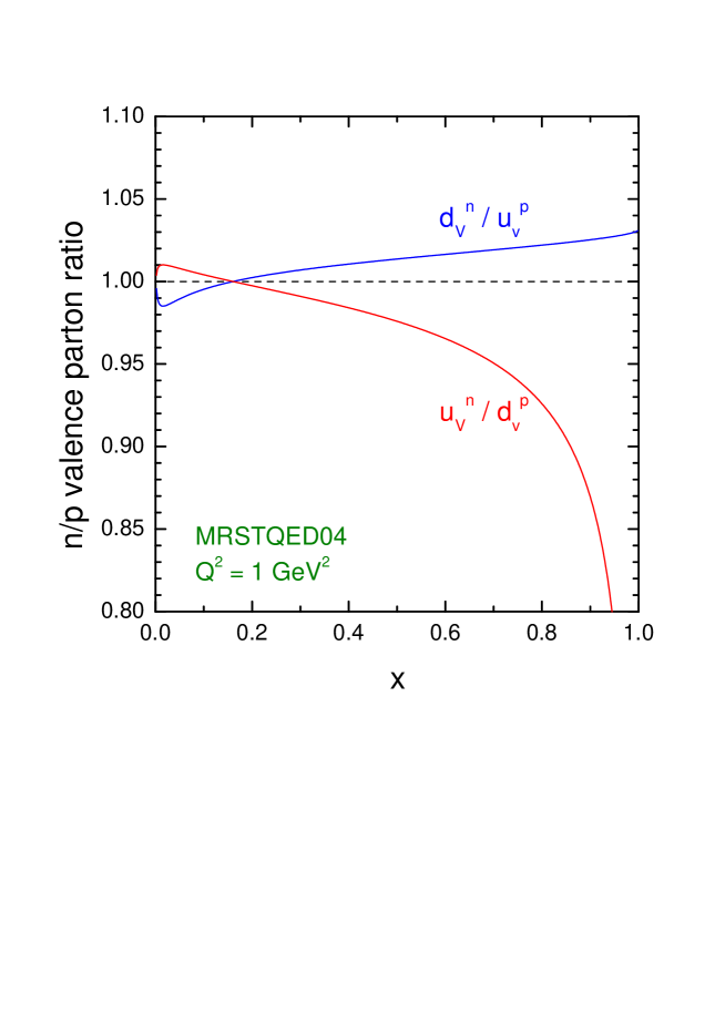
Figure 1: The ratio of valence quarks in the neutron and proton at the starting scale, $Q_{0}^{2}=1$ GeV², in the NLO global analysis, incorporating the isospin violation described by Eq. (8).

It would be possible to devise other physically motivated models for the differences between $u^{p}_{V}(x,Q_{0}^{2})$ and $d^{n}_{V}(x,Q_{0}^{2})$ and between $d^{p}_{V}(x,Q_{0}^{2})$ and $u^{n}_{V}(x,Q_{0}^{2})$, for example we could estimate the change in a quark distribution between scales $m_{q}^{2}$ and $Q_{0}^{2}$ due to QED evolution to be

$$\Delta q(x,Q_{0}^{2})={\alpha\over 2\pi}\int_{x}^{1}\frac{dy}{y}\tilde{P}_{qq}(y)\;e_{q}^{2}\;q(\frac{x}{y},Q_{0}^{2})\;\log(Q_{0}^{2}/m_{q}^{2})\;,$$ (12)

and make the differences between the input quarks for the proton and the neutron to be consistent with this. The momentum carried by the photon in the proton and neutron could then be determined by the momentum lost by each quark due to this contribution. However, in practice this results in distributions and asymmetries which are very similar to those in our model, with the essential features being identical. The results are actually much more sensitive to issues such as the choice of the values of the quark masses.

4 Global analysis including QED effects

Having defined our procedure for obtaining the QED contribution to the input partons, the strategy for the fitting procedure is then to

• calculate the starting distributions $\gamma^{p}(x,Q_{0}^{2})$ and $\gamma^{n}(x,Q_{0}^{2})$;

• parametrise the proton’s quark and gluon distributions at $Q_{0}^{2}$ in the usual (MRST) way;

• compute $\epsilon$ using Eq. (10);

• calculate the neutron starting quark and gluon distributions at $Q_{0}^{2}$ by assuming isospin symmetry for sea quarks and gluons, and isospin-violating valence distributions given by Eq. (8);

• perform the global fit, using separate DGLAP equations for the proton and neutron partons.

We have performed fits at both NLO and NNLO, where the NNLO fit uses the recently calculated exact NNLO splitting functions [10, 11]. We use the same input data as in the recent MRST2004 study of Ref. [12]. In both cases the QED corrections do not alter the fit quality in any significant way. For the NLO fit with QED corrections the $\chi^{2}$ is actually $\sim 15$ higher than that for the standard NLO fit. This increase comes from two sources. The very small amount of momentum carried by the photon is effectively taken from the gluon – the size of the input quarks being very well fixed by the data. This conflicts with our usual findings that at NLO the gluon would actually like more momentum both at high $x$, in order to fit the jet data, and at moderate $x$ ($\sim 0.1-0.01$), in order to fit the slope of the HERA and NMC structure function data. In order to compensate for this loss of gluon the value of $\alpha_{S}(M_{Z}^{2})$ increases very slightly, by about $0.0002$, but the fit to the H1 data is still worse by about $8-10$ units of $\chi^{2}$. Also, the new mechanism of photon radiation, preferentially from high-$x$ up-quarks, tends to make $F_{2}^{p}(x,Q^{2})$ fall more quickly with $Q^{2}$ at high-$x$, and this is effect is increased by the slight increase in $\alpha_{S}(M_{Z}^{2})$. This makes the fit to the BCDMS proton structure function data $10$ units worse, as this data set prefers a slower fall off with increasing $Q^{2}$. The fit to all other sources of data is actually about $5$ units better than the standard NLO fit, with the fit to deuterium data being very slightly improved in general. The overall increase in $\chi^{2}$, whilst being significant, cannot be taken as evidence that QED effects should be ignored. They are most certainly present. Rather it highlights the minor shortcomings in the NLO QCD fit, most particularly the tensions between the gluon and $\alpha_{S}$.

This conclusion is borne out by the result of the NNLO fit with QED corrections. In this case the $\chi^{2}$ is lower than for the standard NNLO fit, albeit only by 3 units. At NNLO the tensions between the gluon and $\alpha_{S}(M_{Z}^{2})$ are much reduced, and the QED corrections do not cause even minor problems in this respect. Indeed, the value of $\alpha_{S}(M_{Z}^{2})$ is essentially unchanged. The small improvement in $\chi^{2}$ is due to slight improvements in the descriptions of the CCFR $F_{3}(x,Q^{2})$ [13], BCDMS $F_{2}^{d}(x,Q^{2})$ [14] and E866 Drell-Yan hydrogen/deuterium ratio data [15], all of which are sensitive to the isospin violation induced by the QED evolution. In the context of the overall fit, however, these improvements are too small to draw any definite conclusions.

We can also perform the fit making a different assumption about the light-quark masses. In particular, we can take the extreme case of constituent-type quark masses of $300$ MeV for both the up and down quarks. From Eq. (5) it is easy to see that this decreases the momentum carried by the photon at input very significantly, and consequently also decreases the input isospin asymmetry. In this case $\epsilon=0.0074$ at $Q_{0}^{2}$, to be compared with $\epsilon=0.0325$ for the previous (current quark mass) fit. However, the loss of gluon momentum is still generated by the subsequent evolution, and so this procedure only improves the quality of the NLO fit very slightly indeed, giving a $\chi^{2}$ of only $\sim 2$ lower than the previous fit. At NNLO there is also an improvement compared to the current quark mass prescription, but even smaller than at NLO. Hence, there is essentially no evidence from the global fit whether current quark mases or constituent quark masses are preferred. We will return to this distinction between quark masses later.

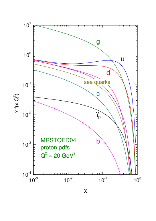
Figure 2: The parton distributions in the proton at $Q^{2}=20\;\rm GeV^{2}$ obtained from the NLO pQCD $+$ LO QED global fit. The curves for the sea quarks correspond to the $\bar{u}$, $\bar{d}$, $s$, $c$ and $b$ distributions.

The parton distributions generated in the fit with the current quark masses, which we will treat as the default fit, are shown in Fig. 2. The quark and gluon distributions are all extremely similar to the standard MRST parton distributions, but it is interesting to note the features of the new photon distribution. At $Q^{2}=20\;\rm GeV^{2}$ it is larger than the $b$-quark distribution, but this is because the $b$ quark is being probed not far above the scale ($Q^{2}=m_{b}^{2}$) where it turns on from zero at NLO. However, the photon distribution is larger than the sea quarks at the highest values of $x$. This is presumably because it is generated directly from the radiation off high-$x$ valence quarks, whereas the sea quarks first branch into gluons which then subsequently produce sea quarks at even smaller momentum fractions. The photon has a similar shape to the sea quarks at small $x$ since it is generated via the splitting function $P_{q\gamma}$ which gives a contribution proportional to the size of the quarks at the smallest $x$ values. In Fig. 3 we show the corresponding figure for the parton distributions in the neutron. The quarks and gluon are almost indistinguishable from those in the proton, once one interchanges up- and down-quark distributions, but the photon distribution is smaller at large $x$, as we would expect from the decreased charge squared of the dominant valence quarks. The photon distributions of the proton and neutron become similar at very small $x$, reflecting the charge symmetry of the small-$x$ sea quarks.

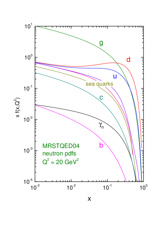
Figure 3: The parton distributions in the neutron at $Q^{2}=20\;\rm GeV^{2}$ obtained from the NLO pQCD $+$ LO QED global fit. The curves for the sea quarks correspond to the $\bar{u}$, $\bar{d}$, $s$, $c$ and $b$ distributions.

Figure 4: The difference between the isospin exchanged valence quarks in the proton and the neutron at $Q^{2}=20\;\rm GeV^{2}$.

In Fig. 4 we plot the valence-quark differences $x(d^{p}_{V}-u^{n}_{V})$ and $x(u^{p}_{V}-d^{n}_{V})$ at $Q^{2}=20\;\rm GeV^{2}$. This figure illustrates the violation of isospin symmetry in the momentum carried by the valence quarks particularly clearly. As mentioned earlier, this has important implications for the anomaly in the measurement of $\sin^{2}\theta_{W}$ reported by NuTeV [7]. The quantity measured, up to corrections due to cuts [7, 18], by NuTeV is

$$R^{-}=\frac{\sigma^{\nu}_{\rm NC}-\sigma^{\bar{\nu}}_{\rm NC}}{\sigma^{\nu}_{\rm CC}-\sigma^{\bar{\nu}}_{\rm CC}}.$$ (13)

In the simplest approximation, i.e. assuming an isoscalar target, no isospin violation and equal strange and anti-strange distributions, this ratio is given by

$$R^{-}\approx\frac{1}{2}-\sin^{2}\theta_{W},$$ (14)

and so the measurement gives a direct determination of $\sin^{2}\theta_{W}$. NuTeV find $\sin^{2}\theta_{W}=0.2277\pm 0.0013\;({\rm stat.})\pm 0.0009\;({\rm syst.})$ [7], compared to the global average of $0.2227\pm 0.0004$, that is, roughly a $3\sigma$ discrepancy. However, if one allows for isospin violation then the simple expression (14) becomes modified to

$$R^{-}=\frac{1}{2}-\sin^{2}\theta_{W}+(1-\frac{7}{3}\sin^{2}\theta_{W})\frac{[\delta U_{\rm v}]-[\delta D_{\rm v}]}{2[V^{-}]},$$ (15)

where

$$[\delta U_{\rm v}]=\int_{0}^{1}dx\,x(u^{p}_{\rm v}(x)-d^{n}_{\rm v}(x)),\qquad\qquad[\delta D_{\rm v}]=\int_{0}^{1}dx\,x(d^{p}_{\rm v}(x)-u^{n}_{\rm v}(x)),$$ (16)

and $[V^{-}]$ is the overall momentum fraction carried by the valence quarks.

In the extraction of the value of $\sin^{2}\theta_{W}$, a correction is made to take account of the electroweak corrections to the cross section. These corrections contain the collinear singularities absorbed into the QED evolution of partons, and so must not be double-counted. The most recent calculations of these corrections [16] do factor out the collinear singularities, and are thus designed to be used with QED-corrected partons. In the electroweak corrections used by NuTeV [17] the collinear singularities were regularised by giving the quarks a mass of $xm_{p}$, which is rather large for the most important region of high $x$, and effectively allows less radiation from high $x$ than low $x$, minimising the isospin-violation effect of QED radiation. Hence, this procedure should be updated, but there is certainly minimal double counting employed by using our QED corrected partons even in this case.

Since the isospin violation generated by the QED evolution is precisely such as to remove more momentum from up-quark distributions than down-quark distributions, it clearly works in the right direction to reduce the NuTeV anomaly. The effect is also $Q^{2}$-dependent, since the quantities in Eq. (16) have a non-zero anomalous dimension. At $Q^{2}=2\;\rm GeV^{2}$ we have $[\delta U_{\rm v}]=-0.002271$, $[\delta D_{\rm v}]=0.001124$ and $[V^{-}]=0.4428$, leading to a change in the measured value of $\sin^{2}\theta_{W}$ of $-0.0018$, i.e. a little more than $1\sigma$ of the total discrepancy is removed. It is not obvious how this result will change with $Q^{2}$, since as $Q^{2}$ increases all the valence distributions evolve to smaller $x$ and the momentum carried by each will decrease. However, the isospin-violating component of the evolution is present, and so we might expect an increase in the effect. Indeed, at $Q^{2}=20\;\rm GeV^{2}$ we find $[\delta U_{\rm v}]=-0.002095$, $[\delta D_{\rm v}]=0.001005$ and $[V^{-}]=0.3501$ leading to a change in measured value of $\sin^{2}\theta_{W}$ of $-0.0021$. This general trend continues with increasing $Q^{2}$, reaching $\Delta\sin^{2}\theta_{W}=-0.0029$ at $Q^{2}=20000\;\rm GeV^{2}$. These results are in remarkable agreement with our previous analysis of isospin-violating effects in parton distributions based on the Lagrange Multiplier method, see Section 5.4 of Ref. [8]. There we found a shift of $\delta R^{-}_{\rm iso}=-0.002$, with 90% confidence level limits of $-0.007<\delta R^{-}_{\rm iso}<+0.007$, comfortably more than needed to explain the NuTeV anomaly.

Hence we conclude that the QED contribution to isospin violation in the valence quarks has a significant effect in reducing the value of $\sin^{2}\theta_{W}$ as measured by NuTeV. We note also that the naive results quoted above need to be corrected for the acceptance cuts made on the data. Functions for convolving with the parton distributions to take these acceptance effects into account are provided in [18]. However these do not contain any $Q^{2}$-dependence, despite accounting in principle for the momentum fraction carried by the valence quarks, which is certainly a scale-dependent quantity. Hence we can only estimate that the corrections may reduce the observed effect by $10-20\%$, see the discussion in Ref. [8]. We also note that the quoted results can be diminished by a factor of up to about 4 if constituent quark masses of $300$ MeV are used instead of current masses – however this option is neither experimentally nor theoretically favoured.

5 Measuring the photon parton distribution, $\gamma(x,Q^{2})$

The photon parton distributions of the proton and neutron, $\gamma^{p}$ and $\gamma^{n}$, are a direct and inescapable consequence of introducing QED contributions into the DGLAP equations. It is therefore interesting to speculate how they could be measured directly in experiment. In particular, such a measurement would test our model assumption for the starting distributions $\gamma(x,Q_{0}^{2})$ given in Eq. (5).

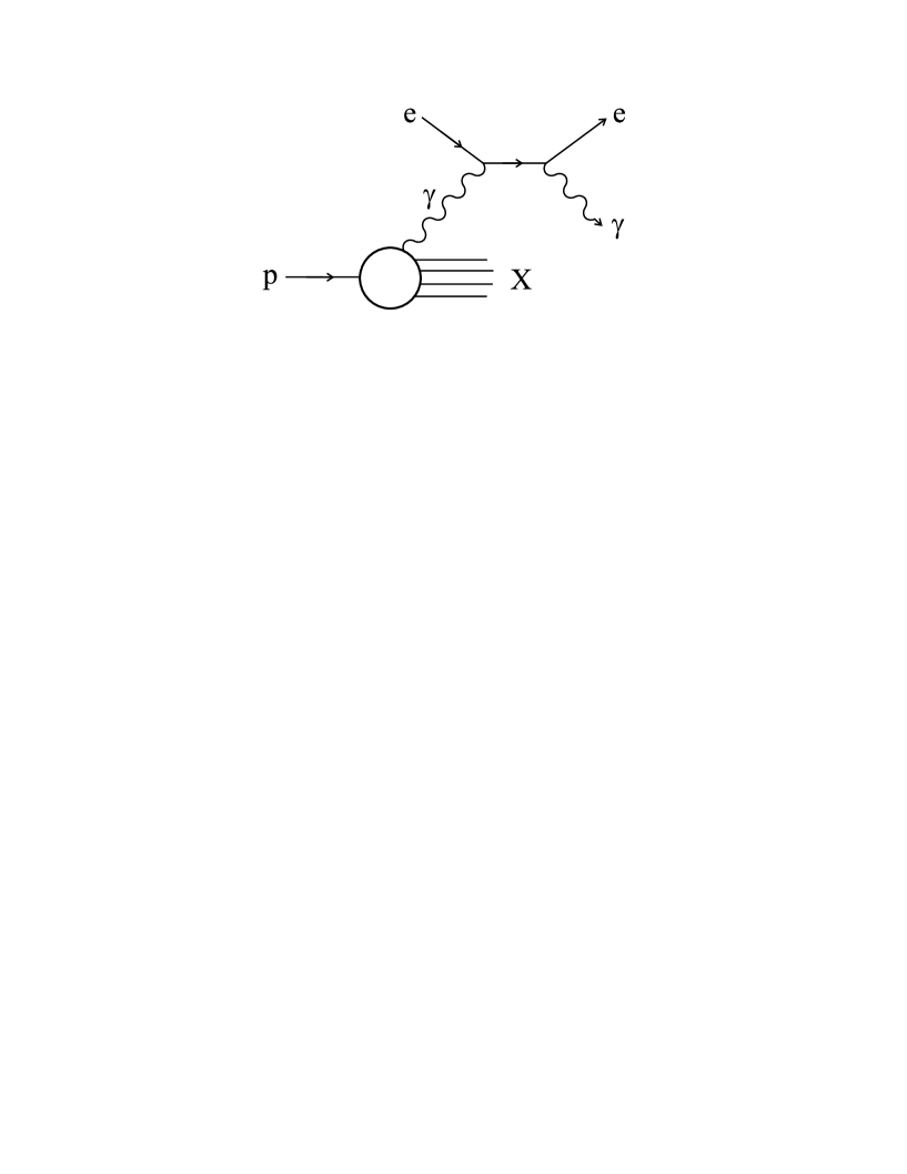
Figure 5: Schematic diagram for the deep inelastic scattering process $ep\to e\gamma X$, which displays the convolution of $\gamma^{p}$ and $\hat{\sigma}(e\gamma\to e\gamma)$ of (17). Besides the $s$-channel diagram for $e\gamma\to e\gamma$ that is shown, there is also a contribution from the diagram with a virtual $u$-channel electron.

The most direct measurement of the photon distribution in the proton would appear to be wide-angle scattering of the photon by a charged lepton beam, thus $ep\to e\gamma X$ where the final state electron and photon are produced with equal and opposite large transverse momentum. The subprocess is then simply QED Compton scattering, $e\gamma\to e\gamma$, and the cross section is obtained by convoluting this subprocess cross section with $\gamma^{p}$, see Fig. 5,

$$\sigma(ep\to e\gamma X)=\int dx^{\gamma}\;\gamma^{p}(x^{\gamma},\mu^{2})\;\hat{\sigma}(e\gamma\to e\gamma)\;,$$ (17)

where $\mu$ is the factorisation scale. If the photon is produced with transverse energy $E_{T}^{\gamma}$ and pseudorapidity $\eta^{\gamma}$ in the HERA laboratory frame, then simple kinematics gives

$$x^{\gamma}={E_{T}^{\gamma}E_{e}\exp(\eta^{\gamma})\over 2E_{p}E_{e}-E_{T}^{\gamma}E_{p}\exp(-\eta^{\gamma})}\;,$$ (18)

where $E_{e}$ and $E_{p}$ are the energies of the electron and proton beams respectively.

The ZEUS collaboration [19] has recently published a measurement of this cross section:

$$\sigma(ep\to e\gamma X)\;=\;5.64\;\pm\;0.58\;\mbox{(stat.)}\;{\small{+0.47\atop-0.72}}\;\mbox{(syst.)}~{}\mbox{pb.}$$ (19)

in electron-proton collisions with $\sqrt{s}=300$ and $318$ GeV. The final state cuts are

$$5<E_{T}^{\gamma}<10\ \mbox{GeV}\;, -0.7<\eta^{\gamma}<0.9\;,$$

$$Q^{2}>35\ \mbox{GeV}^{2}\;, E_{e^{\prime}}>10\ \mbox{GeV}\;,\qquad{139.8}^{\circ}<\theta_{e^{\prime}}<{171.8}^{\circ}\;.$$ (20)

It is noted in [19] that neither PYTHIA nor HERWIG can explain the observed rate (underestimating the measured cross section by factors of 2 and 8 respectively) or (all of) the kinematic distributions in $E_{T}^{\gamma}$, $\eta^{\gamma}$ and $Q^{2}$.

Using the proton’s photon parton distribution obtained in the previous section and using the same cuts as in (20), we find

$$\sigma(ep\to e\gamma X)\;=\;6.2\;\pm\;1.2\ \mbox{pb.}$$ (21)

where the error corresponds to varying the factorisation scale in the range $E_{T}^{\gamma}/2<\mu<2E_{T}^{\gamma}$ with $\mu=E_{T}^{\gamma}$ taken as the central value. The fact that this ‘parameter-free’ prediction agrees well with the experimental data lends strong support to our analysis and, in particular, to our choice of current quark masses in defining the initial photon distribution. As already pointed out, the photon distribution obtained with constituent quark masses is smaller, and in fact reduces the theoretical prediction of (21) to 3.6 pb, in disagreement with the measured value. It would be interesting to extend the ZEUS analysis to make a direct measurement of $\gamma^{p}(x^{\gamma},Q^{2})$ as a function of $x^{\gamma}$, using Eqs. (17,18). In the measurement reported in [19], $x^{\gamma}$ is sampled in a fairly narrow range centred on $x^{\gamma}\simeq 0.005$.

References

-
[1]
U. Baur, S. Keller and D. Wackeroth, Phys. Rev. D59 (1999) 013002;
S. Dittmaier and M. Krämer, Phys. Rev. D65 (2002) 073007;
U. Baur and D. Wackeroth, hep-ph/0405191. - [2] U. Baur, O. Brein, W. Hollik, C. Schappacher and D. Wackeroth, Phys. Rev. D65 (2002) 033007.
- [3] M. L. Ciccolini, S. Dittmaier and M. Kramer, Phys. Rev. D68 (2003) 073003.
-
[4]
A. De Rujula, R. Petronzio and A. Savoy-Navarro, Nucl.
Phys. B154 (1979) 394;
J. Kripfganz and H. Perlt, Zeit. Phys. C41 (1988) 319;
J. Blümlein, Zeit. Phys. C47 (1990) 89. - [5] H. Spiesberger, Phys. Rev. D52 (1995) 4936.
- [6] M. Roth and S. Weinzierl, Phys. Lett. B90 (2004) 190.
- [7] G.P. Zeller et al., Phys. Rev. Lett. 88 (2002) 091802.
- [8] A.D. Martin, R.G. Roberts, W.J. Stirling and R.S. Thorne, Eur. Phys. J. C35 (2004) 325.
- [9] A.D. Martin, R.G. Roberts, W.J. Stirling and R.S. Thorne, presented at the 12th International Workshop on Deep Inelastic Scattering (DIS 2004), hep-ph/0407311.
- [10] S. Moch, J.A.M. Vermaseren and A. Vogt, Nucl. Phys. B688 (2004) 101.
- [11] A. Vogt, S. Moch and J.A.M. Vermaseren, Nucl. Phys. B691 (2004) 129.
- [12] A.D. Martin, R.G. Roberts, W.J. Stirling and R.S. Thorne, hep-ph/0410230.
- [13] CCFR Collaboration: W.G. Seligman et al., Phys. Rev. Lett. 79 (1997) 1213.
- [14] BCDMS Collaboration: A.C. Benvenuti et al., Phys. Lett. B236 (1989) 592.
- [15] E866 Collaboration: R.S. Towell et al., Phys. Rev. D64 (2001) 052002.
-
[16]
K.-P.O. Diener, S. Dittmaier and W. Hollik, Phys. Rev. D69 (2004)
073005;
A.B. Arbuzov, D.Yu. Bardin and L.V. Kalinovskaya, hep-ph/0407203. - [17] D.Yu. Bardin and V.A. Dokuchaeva, JINR E2-86-260 (1986).
- [18] G.P. Zeller et al., Phys. Rev. D65 (2002) 111103; Erratum ibid D67 (2003) 119902.
- [19] ZEUS collaboration: S. Chekanov et al., Phys. Lett. B595 (2004) 86.