The Spin Structure of the Proton

Abstract

This article reviews our present understanding of the QCD spin structure of the proton. We first outline the proton spin puzzle and its possible resolution in QCD. We then review the present and next generation of experiments to resolve the proton’s spin-flavour structure, explaining the theoretical issues involved, the present status of experimental investigation and the open questions and challenges for future investigation.

I INTRODUCTION

Understanding the spin structure of the proton is one of the most challenging problems facing subatomic physics: How is the spin of the proton built up out from the intrinsic spin and orbital angular momentum of its quark and gluonic constituents ? What happens to spin in the transition between current and constituent quarks in low-energy quantum chromodynamics (QCD) ? Key issues include the role of polarized glue and gluon topology in building up the spin of the proton.

The story of the proton’s spin dates from the discovery by Dennison (1927) that the proton is a fermion of spin ${1\over 2}$. Six years later Estermann and Stern (1933) measured the proton’s anomalous magnetic moment, $\kappa_{p}=1.79$ Bohr magnetons, revealing that the proton is not pointlike and has internal structure. The challenge to understand the structure of the proton had begun!

We now understand the proton as a bound state of three confined valence quarks (spin 1/2 fermions) interacting through spin-one gluons, with the gauge group being colour SU(3) Thomas and Weise (2001). The proton is special because of confinement, dynamical chiral symmetry breaking and the very strong colour gauge fields at large distances.

Our present knowledge about the spin structure of the proton at the quark level comes from polarized deep inelastic scattering experiments (pDIS) which use high-energy polarized electrons or muons to probe the structure of a polarized proton and new experiments in semi-inclusive polarized deep inelastic scattering, polarized proton-proton collisions and polarized photoproduction experiments.

The present excitement and global programme in high energy spin physics was inspired by an intriguing discovery in polarized deep inelastic scattering. Following pioneering experiments at SLAC Alguard et al. (1976, 1978); Baum et al. (1983), recent experiments in fully inclusive polarized deep inelastic scattering Windmolders (1999) have extended measurements of the nucleon’s $g_{1}$ spin dependent structure function (the inclusive form-factor measured in these experiments) over a broad kinematic region where one is sensitive to scattering on the valence quarks plus the quark-antiquark sea fluctuations. These experiments have been interpreted to imply that quarks and anti-quarks carry just a small fraction of the proton’s spin (between about 15% and 35%) – less than half the prediction of relativistic constituent quark models ($\sim 60\%$). This result has inspired vast experimental and theoretical activity to understand the spin structure of the proton. Before embarking on a detailed study of the spin structure of the proton it is essential to understand why the small value of this “quark spin content” measured in polarized deep inelastic scattering caused such excitement and why it has so much challenged our understanding of the structure of the proton. We give a brief survey in Section I.A. An outline of the review is given in Section I.B.

Many elements of subatomic physics and quantum field theory are important in our understanding of the proton spin problem. These include:

• the dispersion relations for polarized photon-nucleon scattering,

• Regge theory and the high-energy behaviour of scattering amplitudes,

• the renormalization of the operators which enter the light-cone operator product expansion description of high energy polarized deep inelastic scattering,

• perturbative QCD: the physics of large transverse momentum plus parton model factorization,

• the non-perturbative and non-local topological properties of gluon gauge fields in QCD,

• the role of gluon dynamics in dynamical chiral symmetry breaking (the large mass of the $\eta$ and $\eta^{\prime}$ mesons and the absence of a flavour-singlet pseudoscalar Goldstone boson in spontaneous chiral symmetry breaking).

The purpose of this article is to review our present understanding of the proton spin problem and the physics of the new and ongoing programme aimed at resolving the spin-flavour structure of the nucleon.

I.1 Spin and the proton spin problem

Spin plays an essential role in particle interactions and the fundamental structure of matter, ranging from the subatomic world through to large-scale macroscopic effects in condensed matter physics (e.g. Bose-Einstein condensates, superfluidity, and exotic phases of low temperature ³He) and the structure of dense stars. Spin is essential for the stability of the known Universe. In applications, polarized neutron beams are used to probe the structure of condensed matter and materials systems. Manipulating the spin of the electron may prove to be a key ingredient in designing and constructing a quantum computer – the new field of “spintronics” Zutic et al. (2004).

Spin is the characteristic property of a particle besides its mass and gauge charges. The two invariants of the Poincare group are

$${\cal P}_{\mu}{\cal P}^{\mu} = M^{2}$$

$${\cal W}_{\mu}{\cal W}^{\mu} = -M^{2}s(s+1).$$ (1)

Here ${\cal P}$ and ${\cal W}$ denote the momentum and Pauli-Lubanski spin vectors respectively, $M$ is the particle mass and $s$ denotes its spin. The spin of a particle, whether elementary or composite, determines its equation of motion and its statistics properties. The discovery of spin and its properties are reviewed in Tomonaga (1997) and Martin (2002). Spin ${1\over 2}$ particles are governed by the Dirac equation and Fermi-Dirac statistics whereas spin 0 and spin 1 particles are governed by the Klein-Gordon equation and Bose-Einstein statistics.

The proton’s spin vector $s_{\mu}$ is measured through the forward matrix element of the axial-vector current

$$2Ms_{\mu}=\langle p,s|\ {\overline{\psi}}\gamma_{\mu}\gamma_{5}\psi\ |p,s\rangle$$ (2)

where $\psi$ denotes the proton field operator and $M$ is the proton mass. The quark axial charges

$$2Ms_{\mu}\Delta q=\langle p,s|\ {\overline{q}}\gamma_{\mu}\gamma_{5}q\ |p,s\rangle$$ (3)

then measure information about the quark “spin content” of the proton. (Here $q$ denotes the quark field operator.) The flavour dependent axial charges $\Delta u$, $\Delta d$ and $\Delta s$ can be written as linear combinations of the isovector, SU(3) octet and flavour-singlet axial charges

$$g_{A}^{(3)} = \Delta u-\Delta d$$

$$g_{A}^{(8)} = \Delta u+\Delta d-2\Delta s$$

$$g_{A}^{(0)} = \Delta u+\Delta d+\Delta s.$$ (4)

In semi-classical quark models $\Delta q$ is interpreted as the amount of spin carried by quarks and antiquarks of flavour $q$.

In polarized deep inelastic scattering experiments one measures the nucleon’s $g_{1}$ spin structure function as a function of the Bjorken variable $x$, the fraction of the proton’s momentum which carried by quark, antiquark and gluon partons in incoherent photon-parton scattering with the proton boosted to an infinite momentum frame. From the first moment of $g_{1}$, these experiments have been interpreted to imply a small value for the flavour-singlet axial-charge:

$$g_{A}^{(0)}\bigr{|}_{\rm pDIS}=0.15-0.35.$$ (5)

When combined with the octet axial charge measured in hyperon beta-decays ($g_{A}^{(8)}=0.58\pm 0.03$) it corresponds to a negative strange-quark polarization

$$\Delta s=-0.10\pm 0.04$$ (6)

– that is, polarized in the opposite direction to the spin of the proton.

The Goldberger-Treiman relation relates the isovector axial charge $g_{A}^{(3)}$ to the product of the pion decay constant $f_{\pi}$ and the pion-nucleon coupling constant $g_{\pi NN}$, viz.

$$2Mg_{A}^{(3)}=f_{\pi}g_{\pi NN}$$ (7)

through spontaneously broken chiral symmetry Adler and Dashen (1968). The Goldberger-Treiman relation leads immediately to the result that the spin structure of the proton is related to the dynamics of chiral symmetry breaking.

What happens to gluonic degrees of freedom ? The axial anomaly, a fundamental property of quantum field theory, tells us that the axial-vector current which measures the quark “spin content” of the proton cannot be treated independently of the gluon fields that the quarks live in and that the quark “spin content” is linked to the physics of dynamical axial U(1) symmetry breaking in the flavour-singlet channel. For each flavour $q$ the gauge invariantly renormalized axial-vector current satisfies the anomalous divergence equation Adler (1969); Bell and Jackiw (1969)

$$\partial^{\mu}\bigl{(}{\overline{q}}\gamma_{\mu}\gamma_{5}q\bigr{)}=2m{\overline{q}}i\gamma_{5}q+{\alpha_{s}\over 4\pi}G_{\mu\nu}{\tilde{G}}^{\mu\nu}.$$ (8)

Here $m$ denotes the quark mass and ${\alpha_{s}\over 4\pi}G_{\mu\nu}{\tilde{G}}^{\mu\nu}$ is the topological charge density. The anomaly is important in the flavour-singlet channel and intrinsic to $g_{A}^{(0)}$. It cancels in the non-singlet axial-vector currents which define $g_{A}^{(3)}$ and $g_{A}^{(8)}$. In the QCD parton model the anomaly corresponds to physics at the maximum transverse momentum squared Carlitz et al. (1988). The anomaly contribution also involves non-local structure associated with gluon field topology – see Jaffe and Manohar (1990) and Bass (1998, 2003b). In dynamical axial U(1) symmetry breaking the anomaly and gluon topology are associated with the large masses of the $\eta$ and $\eta^{\prime}$ mesons.

What values should we expect for the $\Delta q$ ? First, consider the static quark model. The simple SU(6) proton wavefunction

$$|p\uparrow\rangle = {1\over\sqrt{2}}|u\uparrow(ud)_{S=0}\rangle+{1\over\sqrt{18}}|u\uparrow(ud)_{S=1}\rangle$$ (9)

$$-{1\over 3}|u\downarrow(ud)_{S=1}\rangle-{1\over 3}|d\uparrow(uu)_{S=1}\rangle$$

$$+{\sqrt{2}\over 3}|d\downarrow(uu)_{S=1}\rangle$$

yields the values $g_{A}^{(3)}={5\over 3}$ and $g_{A}^{(8)}=g_{A}^{(0)}=1$.

In relativistic quark models one has to take into account the four-component Dirac spinor $\psi={N\over\sqrt{4\pi}}\biggl{(}{f\atop i\sigma.{\hat{r}}g}\biggr{)}$ where $N$ is a normalization factor. The lower component of the Dirac spinor is p-wave with intrinsic spin primarily pointing in the opposite direction to spin of the nucleon. Relativistic effects renormalize the axial charges obtained from SU(6) by the factor $N^{2}\int drr^{2}(f^{2}-{1\over 3}g^{2})$ with a net transfer of angular momentum from intrinsic spin to orbital angular momentum – see e.g. Jaffe and Manohar (1990).

Relativistic constituent quark models (which do not include gluonic effects associated with the axial anomaly) generally predict values of $g_{A}^{(3)}\simeq 1.25$ and $g_{A}^{(8)}\sim g_{A}^{(0)}\simeq 0.6$. For example, consider the MIT Bag Model. There, $N^{2}\int_{0}^{R}drr^{2}(f^{2}-{1\over 3}g^{2})=0.65$ where $R$ is the Bag radius. This relativistic factor reduces $g_{A}^{(3)}$ from ${5\over 3}$ to 1.09 and $g_{A}^{(0)}$ to 0.65. Centre of mass motion then increases the axial charges by about 20% bringing $g_{A}^{(3)}$ close to its physical value 1.26. Pion cloud effects are also important. In the SU(2) Cloudy Bag model one finds renormalization factors equal to 0.94 for the isovector axial charge and 0.8 for the isosinglet axial charges Schreiber and Thomas (1988) corresponding to a shift of total angular momentum from intrinsic spin into orbital angular momentum. The resultant predictions are $g_{A}^{(3)}\simeq 1.25$ (in agreement with experiment) and $g_{A}^{(0)}=g_{A}^{(8)}\simeq 0.6$. (Note that, at this level, relativistic quark-pion coupling models contain no explicit strange quark or gluon degrees of freedom with the gluonic degrees of freedom understood to be integrated out into the scalar confinement potential.) The model prediction $g_{A}^{(8)}\simeq 0.6$ agrees with the value extracted from hyperon beta-decays [$g_{A}^{(8)}=0.58\pm 0.03$ Close and Roberts (1993)] whereas the Bag model prediction for $g_{A}^{(0)}$ exceeds the measured value of $g_{A}^{(0)}|_{\rm pDIS}$ by a factor of 2-4.

The overall picture of the spin structure of the proton that has emerged from a combination of experiment and theoretical QCD studies can be summarized in the following key observations:

1. Constituent quark model predictions work remarkably well for the isovector part of the nucleon’s $g_{1}$ spin structure function $(g_{1}^{p}-g_{1}^{n})$: both for the first moment $\int_{0}^{1}dx(g_{1}^{p}-g_{1}^{n})\sim{1\over 6}g_{A}^{(3)}$ which is predicted by the Bjorken sum rule Bjorken (1966, 1970) and also over the whole presently measured range of Bjorken $x$ Bass (1999). This includes the SLAC “small $x$” region ($0.02<x<0.1$) – see Section IX.B below – where one would, a priori, not necessarily expect quark model results to apply. Constituent quark model physics seems to be important in the spin structure of the proton probed at deep inelastic $Q^{2}$! Furthermore, one finds the puzzling result that in the presently measured kinematics where accurate data exist the isovector part of $g_{1}$ considerably exceeds the isoscalar part of $g_{1}$ at small Bjorken $x$ – the opposite to what is observed in unpolarized deep inelastic scattering.

2. In the singlet channel the first moment of the $g_{1}$ spin structure function for polarized photon-gluon fusion $(\gamma^{*}g\rightarrow q{\bar{q}})$ receives a negative contribution $-{\alpha_{s}\over 2\pi}$ from $k_{t}^{2}\sim Q^{2}$, where $k_{t}$ is the quark transverse momentum relative to the photon gluon direction and $Q^{2}$ is the virtuality of the hard photon Carlitz et al. (1988). It also receives a positive contribution (proportional to the mass squared of the struck quark or antiquark) from low values of $k_{t}$, $k_{t}^{2}\sim P^{2},m^{2}$ where $P^{2}$ is the virtuality of the parent gluon and $m$ is the mass of the struck quark. The contact interaction ($k_{t}\sim Q$) between the polarized photon and the gluon is flavour-independent. It is associated with the QCD axial anomaly and measures the spin of the target gluon. The mass dependent contribution is absorbed into the quark wavefunction of the nucleon.

3. Gluon topology is associated with gluonic boundary conditions in the QCD vacuum and has the potential to induce a topological contribution to $g_{A}^{(0)}$ associated with Bjorken $x$ equal to zero: topological $x=0$ polarization or, essentially, a spin “polarized condensate” inside a nucleon Bass (1998). This topology term is associated with a potential $J=1$ fixed pole in the real part of the spin dependent part of the forward Compton amplitude and, if finite, is manifest as a “subtraction at infinity” in the dispersion relation for $g_{1}$ Bass (2003b). It is associated with dynamical axial U(1) symmetry breaking in the transition from constituent quarks to current quarks in QCD.

Summarising these observations, QCD theoretical analysis leads to the formula

$$g_{A}^{(0)}=\biggl{(}\sum_{q}\Delta q-3{\alpha_{s}\over 2\pi}\Delta g\biggr{)}_{\rm partons}+{\cal C}_{\infty}.$$ (10)

Here $\Delta g_{\rm partons}$ is the amount of spin carried by polarized gluon partons in the polarized proton and $\Delta q_{\rm partons}$ measures the spin carried by quarks and antiquarks carrying “soft” transverse momentum $k_{t}^{2}\sim P^{2},m^{2}$ where $P$ is a typical gluon virtuality and $m$ is the light quark mass Efremov and Teryaev (1988); Altarelli and Ross (1988); Carlitz et al. (1988); ${\cal C}_{\infty}$ denotes the potential non-perturbative gluon topological contribution which has support only at Bjorken $x$ equal to zero Bass (1998) so that it cannot be directly measured in polarized deep inelastic scattering.

Since $\Delta g\sim 1/\alpha_{s}$ under QCD evolution, the polarized gluon term $[-{\alpha_{s}\over 2\pi}\Delta g]$ in Eq.(10) scales as $Q^{2}\rightarrow\infty$ Efremov and Teryaev (1988); Altarelli and Ross (1988). The polarized gluon contribution corresponds to two-quark-jet events carrying large transverse momentum $k_{t}\sim Q$ in the final state from photon-gluon fusion Carlitz et al. (1988).

The topological term ${\cal C}_{\infty}$ may be identified with a leading twist “subtraction at infinity” in the dispersion relation for $g_{1}$, whence $g_{A}^{(0)}|_{\rm pDIS}$ is identified with $g_{A}^{(0)}-C_{\infty}$ Bass (2003b). It probes the role of gluon topology in dynamical axial U(1) symmetry breaking in the transition from current to constituent quarks in low energy QCD. The deep inelastic measurement of $g_{A}^{(0)}$, Eq.(5), is not necessarily inconsistent with the constituent quark model prediction 0.6 if a substantial fraction of the spin of the constituent quark is associated with gluon topology in the transition from constituent to current quarks (measured in polarized deep inelastic scattering).

A direct measurement of the strange-quark axial-charge, independent of the analysis of polarized deep inelastic scattering data and any possible “subtraction at infinity” correction, could be made using neutrino proton elastic scattering through the axial coupling of the $Z^{0}$ gauge boson. Comparing the values of $\Delta s$ extracted from high-energy polarized deep inelastic scattering and low-energy $\nu p$ elastic scattering will provide vital information about the QCD structure of the proton.

The vital role of quark transverse momentum in the formula (10) means that it is essential to ensure that the theory and experimental acceptance are correctly matched when extracting information from semi-inclusive measurements aimed at disentangling the individual valence, sea and gluonic contributions. For example, recent semi-inclusive measurements Airapetian et al. (2004, 2005a) using a forward detector and limited acceptance at large transverse momentum ($k_{t}\sim Q$) exhibit no evidence for the large negative polarized strangeness polarization extracted from inclusive data and may, perhaps, be more comparable with $\Delta q_{\rm partons}$ than the inclusive measurement (6) which has the polarized gluon contribution included. Further semi-inclusive measurements with increased luminosity and a 4$\pi$ detector would be valuable. On the theoretical side, when assessing models which attempt to explain the proton’s spin structure it is important to look at the transverse momentum dependence of the proposed dynamics plus the model predictions for the shape of the spin structure functions as a function of Bjorken $x$ in addition to the first moment and the nucleon’s axial charges $g_{A}^{(3)}$, $g_{A}^{(8)}$ and $g_{A}^{(0)}$.

New dedicated experiments are planned or underway to map out the spin-flavour structure of the proton and, especially, to measure the amount of spin carried by the valence and sea quarks and by polarized gluons in the polarized proton. These include semi-inclusive polarized deep inelastic scattering (COMPASS at CERN and HERMES at DESY), polarized proton-proton collisions at the world’s first polarized proton-proton collider RHIC Bunce et al. (2000), and future polarized electron-proton collider studies Bass and De Roeck (2002). Experiments at Jefferson Laboratory are mapping out the spin distribution of quarks carrying a large fraction of the proton’s momentum (Bjorken $x$) and promise to yield exciting new information on confinement related dynamics.

Further interesting information about the structure of the proton will come from the study of “transversity” spin distributions Barone et al. (2002). Working in an infinite momentum frame, these observables measure the distribution of spin polarized transverse to the momentum of the proton in a transversely polarized proton. Since rotations and Euclidean boosts commute and a series of boosts can convert a longitudinally polarized nucleon into a transversely polarized nucleon at infinite momentum, it follows that the difference between the transversity and helicity distributions reflects the relativistic character of quark motion in the nucleon. Furthermore, the transversity spin distribution of the nucleon is charge-parity odd ($C=-1$) and therefore valence like (gluons decouple from its QCD evolution equation in contrast to the evolution equation for flavour-singlet quark distribution appearing in $g_{1}$) making a comparison of the different spin dependent distributions most interesting. Studies of transversity sensitive observables in lepton nucleon and polarized proton proton scattering are being performed by the HERMES Airapetian et al. (2005b), COMPASS and RHIC Adams et al. (2004) experiments.

One would also like to measure the parton orbital angular momentum contributions to the proton’s spin. Exclusive measurements of deeply virtual Compton scattering and single meson production at large $Q^{2}$ offer a possible route to the quark and gluon angular momentum contributions through the physics and formalism of generalized parton distributions Ji (1998); Goeke et al. (2001); Diehl (2003). A vigorous programme to study these reactions is being designed and investigated at several major world laboratories.

I.2 Outline

This Review is organized as follows. In the first part (Sections II - VIII) we review the present status of the proton spin problem focussing on the present experimental situation for tests of polarized deep inelastic spin sum-rules and the theoretical understanding of $g_{A}^{(0)}$. In the second part (Sections IX-XII) we give an overview of the present global programme aimed at disentangling the spin-flavour structure of the proton and the exciting prospects for the new generation of experiments aimed at resolving the proton’s internal spin structure. In Sections II and III we give an overview of the derivation of the spin sum-rules for polarized photon-nucleon scattering, detailing the assumptions that are made at each step. Here we explain how these sum rules could be affected by potential subtraction constants (subtractions at infinity) in the dispersion relations for the spin dependent part of the forward Compton amplitude. We next give a brief review of the partonic (Section IV) and possible fixed pole (Section V) contributions to deep inelastic scattering. Fixed poles are well known to play a vital role in the Adler sum-rule for W-boson nucleon scattering Adler (1966) and the Schwinger term sum-rule for the longitudinal structure function measured in unpolarized deep inelastic $ep$ scattering Broadhurst et al. (1973). We explain how fixed poles could, in principle, affect the sum-rules for the first moments of the $g_{1}$ and $g_{2}$ spin structure functions. For example, a subtraction constant correction to the Ellis-Jaffe sum rule for the first moment of the nucleon’s $g_{1}$ spin dependent structure function would follow if there is a constant real term in the spin dependent part of the deeply virtual forward Compton scattering amplitude. Section VI discusses the QCD axial anomaly and its possible role in understanding the first moment of $g_{1}$. The relationship between the spin structure of the proton and chiral symmetry is outlined in Section VII. This first part of the paper concludes with an overview in Section VIII of the different possible explanations of the small value of $g_{A}^{(0)}$ that have been proposed in the literature, how they relate to QCD, and possible future experimental tests which could help clarrify the key issues. We next focus on the new programme to disentangle the proton’s spin-flavour structure and the Bjorken $x$ dependence of the separate valence, sea and gluonic contributions (Section IX), the theory and experimental investigation of transversity observables (Section X), quark orbital angular momentum and exclusive reactions (Section XI) and the $g_{1}$ spin structure function of the polarized photon (Section XII). A summary of key issues and challenging questions for the next generation of experiments is given in Section XIII.

Complementary review articles on the spin structure of the proton, each with a different emphasis, are given in Anselmino et al. (1995), Cheng (1996), Shore (1998), Lampe and Reya (2000), Fillipone and Ji (2001), Jaffe (2001), Barone et al. (2002) and Stoesslein (2002).

II SCATTERING AMPLITUDES

In photon-nucleon scattering the spin dependent structure functions $g_{1}$ and $g_{2}$ are defined through the imaginary part of the forward Compton scattering amplitude. Consider the amplitude for forward scattering of a photon carrying momentum $q_{\mu}$ ($q^{2}=-Q^{2}\leq 0$) from a polarized nucleon with momentum $p_{\mu}$, mass $M$ and spin $s_{\mu}$. Let $J_{\mu}(z)$ denote the electromagnetic current in QCD. The forward Compton amplitude

$$T_{\mu\nu}(q,p)=i\int d^{4}z\ e^{iq.z}\langle p,s|\ T(J_{\mu}(z)J_{\nu}(0))\ |p,s\rangle\\$$ (11)

is given by the sum of spin independent (symmetric in $\mu$ and $\nu$) and spin dependent (antisymmetric in $\mu$ and $\nu$) contributions, viz.

$$T_{\mu\nu}^{S} = {1\over 2}(T_{\mu\nu}+T_{\nu\mu})$$

$$= -T_{1}(g_{\mu\nu}+{q_{\mu}q_{\nu}\over Q^{2}})$$

$$+{1\over M^{2}}T_{2}(p_{\mu}+{p.q\over Q^{2}}q_{\mu})(p_{\nu}+{p.q\over Q^{2}}q_{\nu})$$

and

$$T_{\mu\nu}^{A} = {1\over 2}(T_{\mu\nu}-T_{\nu\mu})$$

$$= {i\over M^{2}}\epsilon_{\mu\nu\lambda\sigma}q^{\lambda}\biggl{[}s^{\sigma}(A_{1}+{\nu\over M}A_{2})-{1\over M^{2}}s.qp^{\sigma}A_{2}\biggr{]}.$$

Here $\nu=p.q/M$ and $\epsilon_{0123}=+1$; the proton spin vector is normalized to $s^{2}=-1$. The form-factors $T_{1}$, $T_{2}$, $A_{1}$ and $A_{2}$ are functions of $\nu$ and $Q^{2}$.

The hadron tensor for inclusive photon nucleon scattering which contains the spin dependent structure functions is obtained from the imaginary part of $T_{\mu\nu}$

$$W_{\mu\nu}={1\over\pi}{\rm Im}T_{\mu\nu}={1\over 2\pi}\int d^{4}z\ e^{iq.z}\langle p,s|\ [J_{\mu}(z),J_{\nu}(0)]\ |p,s\rangle.$$ (14)

Here the connected matrix element is understood (indicating that the photon interacts with the target and not the vacuum). The spin independent and spin dependent components of $W_{\mu\nu}$ are

$$W_{\mu\nu}^{S}=-W_{1}(g_{\mu\nu}+{q_{\mu}q_{\nu}\over Q^{2}})+{1\over M^{2}}W_{2}(p_{\mu}+{p.q\over Q^{2}}q_{\mu})(p_{\nu}+{p.q\over Q^{2}}q_{\nu})$$ (15)

and

$$W_{\mu\nu}^{A}={i\over M^{2}}\epsilon_{\mu\nu\lambda\sigma}q^{\lambda}\biggl{[}s^{\sigma}(G_{1}+{\nu\over M}G_{2})-{1\over M^{2}}s.qp^{\sigma}G_{2}\biggr{]}$$ (16)

respectively. The structure functions contain all of the target dependent information in the deep inelastic process.

The cross sections for the absorption of a transversely polarized photon with spin polarized parallel $\sigma_{3\over 2}$ and anti-parallel $\sigma_{1\over 2}$ to the spin of the (longitudinally polarized) target nucleon are

$$\sigma_{3\over 2} = {4\pi^{2}\alpha\over\sqrt{\nu^{2}+Q^{2}}}\biggl{[}W_{1}-{\nu\over M^{2}}G_{1}+{Q^{2}\over M^{3}}G_{2}\biggr{]}$$

$$\sigma_{1\over 2} = {4\pi^{2}\alpha\over\sqrt{\nu^{2}+Q^{2}}}\biggl{[}W_{1}+{\nu\over M^{2}}G_{1}-{Q^{2}\over M^{3}}G_{2}\biggr{]},$$

where we use usual conventions for the virtual photon flux factor Roberts (1990). The spin dependent and spin independent parts of the inclusive photon nucleon cross section are

$$\sigma_{1\over 2}-\sigma_{3\over 2}={8\pi^{2}\alpha\over\sqrt{\nu^{2}+Q^{2}}}\biggl{[}{\nu\over M^{2}}G_{1}-{Q^{2}\over M^{3}}G_{2}\biggr{]}$$ (18)

and

$$\sigma_{1\over 2}+\sigma_{3\over 2}={8\pi^{2}\alpha\over\sqrt{\nu^{2}+Q^{2}}}W_{1}.$$ (19)

The $G_{2}$ spin structure function decouples from polarized photoproduction. For real photons ($Q^{2}=0$) one finds the equation $\sigma_{1\over 2}-\sigma_{3\over 2}={8\pi^{2}\alpha\over M^{2}}G_{1}$. The cross section for the absorption of a longitudinally polarized photon is

$$\sigma_{0}={4\pi^{2}\alpha\over\sqrt{\nu^{2}+Q^{2}}}W_{L}={4\pi^{2}\alpha\over\sqrt{\nu^{2}+Q^{2}}}\biggl{[}\biggl{\{}1+{\nu^{2}\over Q^{2}}\biggr{\}}W_{2}-W_{1}\biggr{]}.$$ (20)

The $W_{2}$ structure function is measured in unpolarized lepton nucleon scattering through the absorption of transversely and longitudinally polarized photons.

Our present knowledge about the high-energy spin structure of the nucleon comes from polarized deep inelastic scattering experiments. These experiments involve scattering a high-energy charged lepton beam from a nucleon target at large momentum transfer squared. One measures the inclusive cross-section. The lepton beam (electrons at DESY, JLab and SLAC and muons at CERN) is longitudinally polarized. The nucleon target may be either longitudinally or transversely polarized.

The relation between deep inelastic lepton nucleon cross-sections and the virtual-photon nucleon cross-sections discussed above is discussed and derived in various textbooks – e.g. Roberts (1990). Polarized deep inelastic scattering experiments have so far all been performed using a fixed target. Consider polarized $ep$ scattering. We specialize to the target rest frame and let $E$ denote the energy of the incident electron which is scattered through an angle $\theta$ to emerge in the final state with energy $E^{\prime}$. Let $\uparrow\downarrow$ denote the longitudinal polarization of the electron beam. For a longitudinally polarized proton target (with spin denoted $\Uparrow\Downarrow$) the unpolarized and polarized differential cross-sections are

$$\Biggl{(}{d^{2}\sigma\uparrow\Downarrow\over d\Omega dE^{{}^{\prime}}} + {d^{2}\sigma\uparrow\Uparrow\over d\Omega dE^{{}^{\prime}}}\Biggr{)}$$

$$= {\alpha^{2}\over 4E^{2}\sin^{4}{\theta\over 2}}\biggl{[}2\sin^{2}{\theta\over 2}\ W_{1}+\cos^{2}{\theta\over 2}\ W_{2}\biggr{]}$$

and

$$\Biggl{(}{d^{2}\sigma\uparrow\Downarrow\over d\Omega dE^{{}^{\prime}}} - {d^{2}\sigma\uparrow\Uparrow\over d\Omega dE^{{}^{\prime}}}\Biggr{)}$$

$$= {4\alpha^{2}\over M^{3}Q^{2}}\ {E^{{}^{\prime}}\over E}\ \biggl{[}M(E+E^{{}^{\prime}}\cos\theta)\ G_{1}-Q^{2}\ G_{2}\biggr{]}.$$

For a target polarized transverse to the electron beam the spin dependent part of the differential cross-section is

$$\Biggl{(}{d^{2}\sigma\uparrow\Rightarrow\over d\Omega dE^{{}^{\prime}}}-{d^{2}\sigma\uparrow\Leftarrow\over d\Omega dE^{{}^{\prime}}}\Biggr{)}={4\alpha^{2}\over M^{3}Q^{2}}{E^{{}^{\prime}2}\over E}\sin\theta\biggl{[}M\ G_{1}+2E\ G_{2}\biggr{]}.$$ (23)

II.1 Scaling and polarized deep inelastic scattering

In high $Q^{2}$ deep inelastic scattering the structure functions exhibit approximate scaling. One finds

$$M\ W_{1}(\nu,Q^{2}) \rightarrow F_{1}(x,Q^{2})$$

$$\nu\ W_{2}(\nu,Q^{2}) \rightarrow F_{2}(x,Q^{2})$$

$${\nu\over M}\ G_{1}(\nu,Q^{2}) \rightarrow g_{1}(x,Q^{2})$$

$${\nu^{2}\over M^{2}}\ G_{2}(\nu,Q^{2}) \rightarrow g_{2}(x,Q^{2}).$$ (24)

The structure functions $F_{1}$, $F_{2}$, $g_{1}$ and $g_{2}$ are to a very good approximation independent of $Q^{2}$ and depend only on $x$. (The small $Q^{2}$ dependence which is present in these structure functions is logarithmic and determined by perturbative QCD evolution.) Substituting (24) in the cross-section formula (LABEL:eqb22) for the longitudinally polarized target one finds that the $g_{2}$ contribution to the differential cross section and the longitudinal spin asymmetry is suppressed relative to the $g_{1}$ contribution by the kinematic factor ${M\over E}\sim 0$, viz.

$${\cal A}_{1}={\sigma_{1\over 2}-\sigma_{3\over 2}\over\sigma_{1\over 2}+\sigma_{3\over 2}}={M\nu G_{1}-Q^{2}G_{2}\over M^{3}W_{1}}={g_{1}-{Q^{2}\over\nu^{2}}\ g_{2}\over F_{1}}\rightarrow{g_{1}\over F_{1}}.$$

(25)

For a transverse polarized target this kinematic suppression factor for $g_{2}$ is missing meaning that transverse polarization is vital to measure $g_{2}$. We refer to Roberts (1990) and Windmolders (2002) for the procedure how the spin dependent structure functions are extracted from the spin asymmetries measured in polarized deep inelastic scattering.

In the (pre-QCD) parton model the deep inelastic structure functions $F_{1}$ and $F_{2}$ are written as

$$F_{1}(x)={1\over 2x}F_{2}(x)={1\over 2}\sum_{q}e_{q}^{2}\{q+{\bar{q}}\}(x)$$ (26)

and the polarized structure function $g_{1}$ is

$$g_{1}(x)={1\over 2}\sum_{q}e_{q}^{2}\Delta q(x).$$ (27)

Here $e_{q}$ denotes the electric charge of the struck quark and

$$\{q+{\bar{q}}\}(x) = (q^{\uparrow}+{\overline{q}}^{\uparrow})(x)+(q^{\downarrow}+{\overline{q}}^{\downarrow})(x)$$

$$\Delta q(x) = (q^{\uparrow}+{\overline{q}}^{\uparrow})(x)-(q^{\downarrow}+{\overline{q}}^{\downarrow})(x)$$

denote the spin-independent (unpolarized) and spin-dependent quark parton distributions which measure the distribution of quark momentum and spin in the proton. For example, ${\overline{q}}^{\uparrow}(x)$ is interpreted as the probability to find an anti-quark of flavour $q$ with plus component of momentum $xp_{+}$ ($p_{+}$ is the plus component of the target proton’s momentum) and spin polarized in the same direction as the spin of the target proton. When we integrate out the momentum fraction $x$ the quantity $\Delta q=\int_{0}^{1}dx\ \Delta q(x)$ is interpreted as the fraction of the proton’s spin which is carried by quarks (and anti-quarks) of flavour $q$ – hence the parton model interpretation of $g_{A}^{(0)}$ as the total fraction of the proton’s spin carried by up, down and strange quarks. In QCD the flavour-singlet combination of these quark parton distributions mixes with the spin independent and spin dependent gluon distributions respectively under $Q^{2}$ evolution. The gluon parton distributions measure the momentum and spin dependence of glue in the proton. The second spin structure function $g_{2}$ has a non-trivial parton interpretation Jaffe (1990) and vanishes without the effect of quark transverse momentum – see e.g. Roberts (1990).

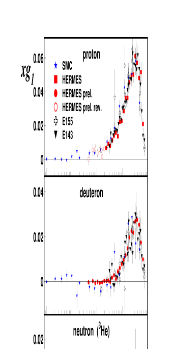
Figure 1: The world data on $xg_{1}$ with data points shown at the $Q^{2}$ they were measured at. Figure courtesy of U. Stoesslein.

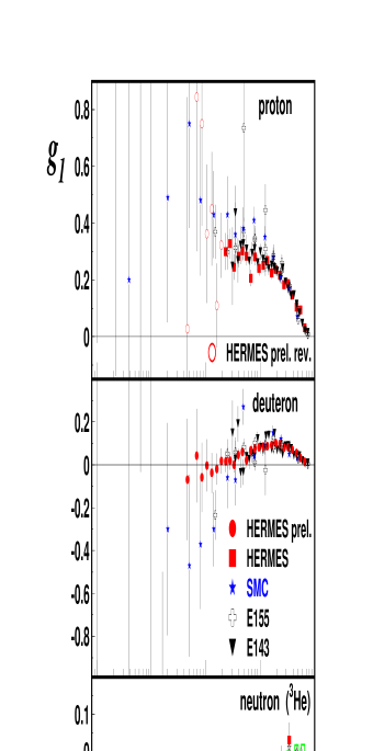
Figure 2: The world data on $g_{1}$ with data points shown at the $Q^{2}$ they were measured at. Figure courtesy of U. Stoesslein.

An overview of the world data on the nucleon’s $g_{1}$ spin structure function is shown in Figure 1 (which shows $xg_{1}$) and Figure 2 (which shows $g_{1}$). There is a general consistency between all data sets. The largest range is provided by the SMC experiment Adeva et al. (1998a, 1999), namely $0.00006<x<0.8$ and $0.02<Q^{2}<100$ GeV². This experiment used proton and deuteron targets with 100-200 GeV muon beams. The final results are given in  Adeva et al. (1998a). The low $x$ data from SMC Adeva et al. (1999) are at a $Q^{2}$ well below 1 GeV², and the asymmetries are found to be compatible with zero. The most precise data comes from the electron scattering experiments at SLAC (E154 on the neutron Abe et al. (1997) and E155 on the proton Anthony et al. (1999, 2000)), JLab Zheng et al. (2004a, b) (on the neutron) and HERMES at DESY Airapetian et al. (1998); Ackerstaff et al. (1997) (on the proton and neutron), with JLab focussed on the large $x$ region. The recipes for extracting the neutron’s spin structure function from experiments using a deuteron or ³He target are discussed in Piller and Weise (2000) and Thomas (2002).

Note the large isovector component in the data at small $x$ (between 0.01 and 0.1) which considerably exceeds the isoscalar component in the measured kinematics. This result is in stark contrast to the situation in the unpolarized structure function $F_{2}$ where the small $x$ region is dominated by isoscalar pomeron exchange. Given the large experimental errors on the data little can presently be concluded about $g_{1}$ at the smallest $x$ values ($x$ less than about 0.006).

The structure function data at different values of $x$ (Figs.1 and 2) are measured at different $Q^{2}$ values in the experiments, viz. $x_{\rm expt.}=x(Q^{2})$. For the ratios $g_{1}/F_{1}$ there is no experimental evidence of $Q^{2}$ dependence in any given $x$ bin. The E155 Collaboration at SLAC found the following good phenomenological fit to their final data set with $Q^{2}>1$GeV² and energy of the hadronic final state $W>2$GeV Anthony et al. (2000):

$${g_{1}^{p}\over F_{1}^{p}} = x^{0.700}(0.817+1.014x-1.489x^{2})\times(1+{c^{p}\over Q^{2}})$$

$${g_{1}^{n}\over F_{1}^{n}} = x^{-0.335}(-0.013-0.330x+0.761x^{2})\times(1+{c^{n}\over Q^{2}}).$$

The coefficients $c^{p}=-0.04\pm 0.06$ and $c^{n}=0.13\pm 0.45$ describing the $Q^{2}$ dependence are found to be small and consistent with zero. The $Q^{2}$ dependence of the $g_{1}$ spin structure function is shown in Fig.3. It is useful to compare data at the same $Q^{2}$, e.g. for the comparison of experimental data with the predictions of deep inelastic sum-rules. To this end, the measured $x$ points are shifted to the same $Q^{2}$ using either the (approximate) $Q^{2}$ independence of the asymmetry or performing next-to-leading-order (NLO) QCD motivated fits Adeva et al. (1998b); Anthony et al. (2000); Gehrmann and Stirling (1996); Altarelli et al. (1997); Glück et al. (2001); Blümlein and Böttcher (2002); Goto et al. (2000); Hirai et al. (2004); Leader et al. (2002) to the measured data and evolving the measured data points all to the same value of $Q^{2}$.

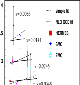
Figure 3: $Q^{2}$ dependence of $g_{1}^{p}$ for $Q^{2}>1$GeV² together with a simple fit according to Anthony et al. (2000) and a NLO perturbative QCD fit from Stoesslein (2002).

II.2 Regge theory and the small $x$ behaviour of spin structure functions

The small $x$ or high energy behaviour of spin structure functions is an important issue both for the extrapolation of data needed to test spin sum rules for the first moment of $g_{1}$ and also in its own right.

Regge theory makes predictions for the high-energy asymptotic behaviour of the structure functions:

$$W_{1} \sim\nu^{\alpha}$$ (30)

$$W_{2} \sim\nu^{\alpha-2}$$

$$G_{1} \sim\nu^{\alpha-1}$$

$$G_{2} \sim\nu^{\alpha-1}.$$

Here $\alpha$ denotes the (effective) intercept for the leading Regge exchange contributions. The Regge predictions for the leading exchanges include $\alpha=1.08$ for the pomeron contributions to $W_{1}$ and $W_{2}$, and $\alpha\simeq 0.5$ for the $\rho$ and $\omega$ exchange contributions to the spin independent structure functions.

For $G_{1}$ the leading gluonic exchange behaves as $\{\ln\nu\}/\nu$ Close and Roberts (1994); Bass and Landshoff (1994). In the isovector and isoscalar channels there are also isovector $a_{1}$ and isoscalar $f_{1}$ Regge exchanges plus contributions from the pomeron-$a_{1}$ and pomeron-$f_{1}$ cuts Heimann (1973). If one makes the usual assumption that the $a_{1}$ and $f_{1}$ Regge trajectories are straight lines parallel to the $(\rho,\omega)$ trajectories then one finds $\alpha_{a_{1}}\simeq\alpha_{f_{1}}\simeq-0.4$, within the phenomenological range $-0.5\leq\alpha_{a_{1}}\leq 0$ discussed in Ellis and Karliner (1988). Taking the masses of the $a_{1}(1260)$ and $a_{3}(2070)$ states plus the $a_{1}(1640)$ and $a_{3}(2310)$ states from the Particle Data Group (2004) yields two parallel $a_{1}$ trajectories with slope $\sim 0.75$GeV^-2 and a leading trajectory with slightly lower intercept: $\alpha_{a_{1}}\simeq-0.18$.

For this value of the $a_{1}$ intercept the effective intercepts corresponding to the soft-pomeron $a_{1}$ cut and the hard-pomeron $a_{1}$ cut are $\simeq-0.1$ and $\simeq+0.25$ respectively if one takes the soft and hard pomerons as two distinct exchanges Cudell et al. (1999) . In the framework of the Donnachie-Landshoff-Nachtmann model of soft pomeron physics Landshoff and Nachtmann (1987); Donnachie and Landshoff (1988) the logarithm in the ${\ln\nu\over\nu}$ contribution comes from the region of internal momentum where two non-perturbative gluons are radiated collinear with the proton Bass and Landshoff (1994).

For $G_{2}$ one expects contributions from possible multi-pomeron (three or more) cuts ($\sim(\ln\nu)^{-5}$) and Regge-pomeron cuts ($\sim\nu^{\alpha_{i}(0)-1}/\ln\nu$) with $\alpha_{i}(0)<1$ (since the pomeron does not couple to $A_{1}$ or $A_{2}$ as a single gluonic exchange) – see Ioffe et al. (1984).

In terms of the scaling structure functions of deep inelastic scattering the relations (30) become

$$F_{1} \sim{1\over x}^{\alpha}$$ (31)

$$F_{2} \sim{1\over x}^{\alpha-1}$$

$$g_{1} \sim{1\over x}^{\alpha}$$

$$g_{2} \sim{1\over x}^{\alpha+1}.$$

For deep inelastic values of $Q^{2}$ there is some debate about the application of Regge arguments. In the conventional approach the effective intercepts for small $x$, or high $\nu$, physics tend to increase with increasing $Q^{2}$ through perturbative QCD evolution which acts to shift the weight of the structure functions to smaller $x$. The polarized isovector combination $g_{1}^{p}-g_{1}^{n}$ is observed to rise in the small $x$ data from SLAC and SMC like $\sim x^{-0.5}$ although it should be noted that, in the measured $x$ range, this exponent could be softened through multiplication by a $(1-x)^{n}$ factor – for example associated with perturbative QCD counting rules at large $x$ ($x$ close to one). For example, the exponent $x^{-0.5}$ could be modified to about $x^{-0.25}$ through multiplication by a factor $(1-x)^{6}$. In an alternative approach Cudell et al. (1999) have argued that the Regge intercepts should be independent of $Q^{2}$ and that the “hard pomeron” revealed in unpolarized deep inelastic scattering at HERA is a distinct exchange independent of the soft pomeron which should also be present in low $Q^{2}$ photoproduction data.

Detailed investigation of spin dependent Regge theory and the low $x$ behaviour of spin structure functions could be performed at SLAC or using a future polarized $ep$ collider (e-RHIC) where measurements could be obtained through a broad range of $Q^{2}$ from photoproduction through the “transition region” to polarized deep inelastic scattering. These measurements would provide a baseline for investigations of perturbative QCD motivated small $x$ behaviour in $g_{1}$. Open questions include: Does the rise in $g_{1}^{p}-g_{1}^{n}$ at small Bjorken $x$ persist to small values of $Q^{2}$ ? How does this rise develop as a function of $Q^{2}$ ? Further possible exchange contributions in the flavour-singlet sector associated with polarized glue could also be looked for. For example, colour coherence predicts that the ratio of polarized to unpolarized gluon distributions $\Delta g(x)/g(x)\propto x$ as $x\rightarrow 0$ Brodsky et al. (1995) suggesting that, perhaps, there is a spin analogue of the hard pomeron with intercept about 0.45 corresponding to the polarized gluon distribution.

The $s$ and $t$ dependence of spin dependent Regge theory is being investigated by the pp2pp experiment Bültmann et al. (2003) at RHIC which is studying polarized proton proton elastic scattering at centre of mass energies $50<\sqrt{s}<500$GeV and four momentum transfer $0.0004<|t|<1.3$GeV².

III DISPERSION RELATIONS AND SPIN SUM RULES

Sum rules for the (spin) structure functions measured in deep inelastic scattering are derived using dispersion relations and the operator product expansion. For fixed $Q^{2}$ the forward Compton scattering amplitude $T_{\mu\nu}(\nu,Q^{2})$ is analytic in the photon energy $\nu$ except for branch cuts along the positive real axis for $|\nu|\geq Q^{2}/2M$. Crossing symmetry implies that

$$A_{1}^{*}(Q^{2},-\nu) = A_{1}(Q^{2},\nu)$$

$$A_{2}^{*}(Q^{2},-\nu) = -A_{2}(Q^{2},\nu).$$ (32)

The spin structure functions in the imaginary parts of $A_{1}$ and $A_{2}$ satisfy the crossing relations

$$G_{1}(Q^{2},-\nu) = -G_{1}(Q^{2},\nu)$$

$$G_{2}(Q^{2},-\nu) = +G_{2}(Q^{2},\nu).$$ (33)

For $g_{1}$ and $g_{2}$ these relations become

$$g_{1}(x,Q^{2}) = +g_{1}(-x,Q^{2})$$

$$g_{2}(x,Q^{2}) = +g_{2}(-x,Q^{2}).$$ (34)

We use Cauchy’s integral theorem and the crossing relations to derive dispersion relations for $A_{1}$ and $A_{2}$. Assuming that the asymptotic behaviour of the spin structure functions $G_{1}$ and $G_{2}$ yield convergent integrals we are tempted to write the two unsubtracted dispersion relations:

$$A_{1}(Q^{2},\nu) = {2\over\pi}\int_{Q^{2}/2M}^{\infty}\ {\nu^{\prime}d\nu^{\prime}\over\nu^{\prime 2}-\nu^{2}}\ {\rm Im}A_{1}(Q^{2},\nu^{\prime})$$

$$A_{2}(Q^{2},\nu) = {2\over\pi}\nu\int_{Q^{2}/2M}^{\infty}\ {d\nu^{\prime}\over\nu^{\prime 2}-\nu^{2}}\ {\rm Im}A_{2}(Q^{2},\nu^{\prime}).$$

These expressions can be rewritten as dispersion relations involving $g_{1}$ and $g_{2}$. We define:

$$\alpha_{1}(\omega,Q^{2}) = {\nu\over M}\ A_{1}$$

$$\alpha_{2}(\omega,Q^{2}) = {\nu^{2}\over M^{2}}\ A_{2}.$$ (36)

Then, the formulae in (LABEL:eqc35) become

$$\alpha_{1}(\omega,Q^{2}) = 2\omega\int_{1}^{\infty}\ {d\omega^{\prime}\over\omega^{\prime 2}-\omega^{2}}\ g_{1}(\omega^{\prime},Q^{2})$$

$$\alpha_{2}(\omega,Q^{2}) = 2\omega^{3}\int_{1}^{\infty}\ {d\omega^{\prime}\over\omega^{\prime 2}(\omega^{\prime 2}-\omega^{2})}\ g_{2}(\omega^{\prime},Q^{2})$$

where $\omega={1\over x}={2M\nu\over Q^{2}}$.

In general there are two alternatives to an unsubtracted dispersion relation.

1. First, if the high energy behaviour of $G_{1}$ and/or $G_{2}$ (at some fixed $Q^{2}$) produced a divergent integral, then the dispersion relation would require a subtraction. Regge predictions for the high energy behaviour of $G_{1}$ and $G_{2}$ – see Eq.(30) – each lead to convergent integrals so this scenario is not expected to occur, even after including the possible effects of QCD evolution.

2. Second, even if the integral in the unsubtracted relation converges, there is still the potential for a “subtraction at infinity”. This scenario would occur if the real part of $A_{1}$ and/or $A_{2}$ does not vanish sufficiently fast enough when $\nu\rightarrow\infty$ so that we pick up a finite contribution from the contour (or “circle at infinity”). In the context of Regge theory such subtractions can arise from fixed poles (with $J=\alpha(t)=0$ in $A_{2}$ or $J=\alpha(t)=1$ in $A_{1}$ for all $t$) in the real part of the forward Compton amplitude. We shall discuss these fixed poles and potential subtractions in Section V.

In the presence of a potential “subtraction at infinity” the dispersion relations (LABEL:eqc35) are modified to:

$$A_{1}(Q^{2},\nu) = {\cal P}_{1}(\nu,Q^{2})$$

$$\ \ \ \ \ +{2\over\pi}\int_{Q^{2}/2M}^{\infty}\ {\nu^{\prime}d\nu^{\prime}\over\nu^{\prime 2}-\nu^{2}}\ {\rm Im}A_{1}(q^{2},\nu^{\prime})$$

$$A_{2}(Q^{2},\nu) = {\cal P}_{2}(\nu,Q^{2})$$

$$\ \ \ \ \ +{2\over\pi}\nu\int_{Q^{2}/2M}^{\infty}\ {d\nu^{\prime}\over\nu^{\prime 2}-\nu^{2}}\ {\rm Im}A_{2}(q^{2},\nu^{\prime}).$$

Here ${\cal P}_{1}(\nu,Q^{2})$ and ${\cal P}_{2}(\nu,Q^{2})$ denote the subtraction constants. Factoring out the $\nu$ dependence of these subtraction constants, we define two $\nu$ independent quantities $\beta_{1}(Q^{2})$ and $\beta_{2}(Q^{2})$:

$${\cal P}_{1}(\nu,Q^{2}) = \beta_{1}(Q^{2})$$

$${\cal P}_{2}(\nu,Q^{2}) = \beta_{2}(Q^{2}){M\over\nu}.$$ (39)

The crossing relations (32) for $A_{1}$ and $A_{2}$ are observed by the functions ${\cal P}_{i}$. Scaling requires that $\beta_{1}(Q^{2})$ and $\beta_{2}(Q^{2})$ (if finite) must be nonpolynomial in $Q^{2}$ – see Section V. The equations (LABEL:eqc38) can be rewritten:

$$\alpha_{1}(\omega,Q^{2}) = {Q^{2}\over 2M^{2}}\ \beta_{1}(Q^{2})\ \omega+$$

$$2\omega\int_{1}^{\infty}\ {d\omega^{\prime}\over\omega^{\prime 2}-\omega^{2}}\ g_{1}(\omega^{\prime},Q^{2})$$

$$\alpha_{2}(\omega,Q^{2}) = {Q^{2}\over 2M^{2}}\ \beta_{2}(Q^{2})\ \omega+$$

$$2\omega^{3}\int_{1}^{\infty}\ {d\omega^{\prime}\over\omega^{\prime 2}(\omega^{\prime 2}-\omega^{2})}\ g_{2}(\omega^{\prime},Q^{2}).$$

Next, the fact that both $\alpha_{1}$ and $\alpha_{2}$ are analytic for $|\omega|\leq 1$ allows us to make the Taylor series expansions (about $\omega=0$)

$$\alpha_{1}(x,Q^{2}) = {Q^{2}\over 2M^{2}}\ \beta_{1}(Q^{2})\ {1\over x}$$

$$+{2\over x}\sum_{n=0,2,4,..}\biggl{(}{1\over x^{n}}\biggr{)}\int_{0}^{1}dy\ y^{n}g_{1}(y,Q^{2})$$

$$\alpha_{2}(x,Q^{2}) = {Q^{2}\over 2M^{2}}\ \beta_{2}(Q^{2})\ {1\over x}$$

$$+{2\over x^{3}}\sum_{n=0,2,4,..}\biggl{(}{1\over x^{n}}\biggr{)}\int_{0}^{1}dy\ y^{n+2}g_{2}(y,Q^{2})$$

with $x={1\over\omega}$.

These equations form the basis for the spin sum rules for polarized photon nucleon scattering. We next outline the derivation of the Bjorken Bjorken (1966, 1970) and Ellis-Jaffe Ellis and Jaffe (1974) sum rules for the isovector and flavour-singlet parts of $g_{1}$ in polarized deep inelastic scattering, the Burkhardt-Cottingham sum rule for $G_{2}$ Burkhardt and Cottingham (1970), and the Gerasimov-Drell-Hearn sum rule for polarized photoproduction Gerasimov (1965); Drell and Hearn (1966). Each of these spin sum rules assumes no subtraction at infinity.

III.1 Deep inelastic spin sum rules

Sum rules for polarized deep inelastic scattering are derived by combining the dispersion relation expressions (LABEL:eqc41) with the light cone operator production expansion. When $Q^{2}\rightarrow\infty$ the leading contribution to the spin dependent part of the forward Compton amplitude comes from the nucleon matrix elements of a tower of gauge invariant local operators multiplied by Wilson coefficients, viz.

$$T_{\mu\nu}^{A} = i\epsilon_{\mu\nu\lambda\sigma}q^{\lambda}\sum_{n=0,2,4,..}\biggl{(}-{2\over q^{2}}\biggr{)}^{n+1}q^{\mu_{1}}q^{\mu_{2}}...q^{\mu_{n}}$$

$$\ \ \ \ \ \ \ \ \ \ \ \ \ \ \ \sum_{i=q,g}\Theta^{(i)}_{\sigma\{\mu_{1}...\mu_{n}\}}E^{i}_{n}({Q^{2}\over\mu^{2}},\alpha_{s})$$

where

$$\Theta^{(q)}_{\sigma\{\mu_{1}...\mu_{n}\}}\equiv i^{n}\bar{\psi}\gamma_{\sigma}\gamma_{5}D_{\{\mu_{1}}...D_{\mu_{n}\}}\psi-{\rm traces}$$ (43)

and

$$\Theta^{(g)}_{\sigma\{\mu_{1}...\mu_{n}\}}\equiv i^{n-1}\epsilon_{\alpha\beta\gamma\sigma}G^{\beta\gamma}D_{\{\mu_{1}}...D_{\mu_{n-1}}G_{\ \mu_{n}\}}^{\alpha}-{\rm traces}$$ (44)

are local operators. Here $D_{\mu}=\partial_{\mu}+igA_{\mu}$ is the gauge covariant derivative and the sum over even values of $n$ in Eq.(LABEL:eqc42) reflects the crossing symmetry properties of $T_{\mu\nu}$. The functions $E^{q}_{n}({Q^{2}\over\mu^{2}},\alpha_{s})$ and $E^{g}_{n}({Q^{2}\over\mu^{2}},\alpha_{s})$ are the respective Wilson coefficients. (Note that, for simplicity, in this discussion we consider the case of a single quark flavour with unit charge and zero quark mass. The results quoted in Section III.B below include the extra steps of using the full electromagnetic current in QCD.)

The operators in Eq.(LABEL:eqc42) may each be written as the sum of a totally symmetric operator and an operator with mixed symmetry

$$\Theta_{\sigma\{\mu_{1}...\mu_{n}\}}=\Theta_{\{\sigma\mu_{1}...\mu_{n}\}}+\Theta_{[\sigma,\{\mu_{1}]...\mu_{n}\}}.$$ (45)

These operators have the matrix elements:

$$\langle p,s|\Theta_{\{\sigma\mu_{1}...\mu_{n}\}}|p,s\rangle$$

$$\ \ \ \ \ \ \ =\{s_{\sigma}p_{\mu_{1}}...p_{\mu_{n}}+s_{\mu_{1}}p_{\sigma}p_{\mu_{2}}...p_{\mu_{n}}+...\}{a_{n}\over n+1}$$

$$\langle p,s|\Theta_{[\{\sigma\mu_{1}]...\mu_{n}\}}|p,s\rangle$$

$$\ \ \ \ \ \ \ =\{(s_{\sigma}p_{\mu_{1}}-s_{\mu_{1}}p_{\sigma})p_{\mu_{2}}...p_{\mu_{n}}$$

$$\ \ \ \ \ \ \ \ \ \ +(s_{\sigma}p_{\mu_{2}}-s_{\mu_{2}}p_{\sigma})p_{\mu_{1}}...p_{\mu_{n}}+...\}{d_{n}\over n+1}.$$

(46)

Now define ${\tilde{a}}_{n}=a_{n}^{(q)}E_{1n}^{q}+a_{n}^{(g)}E_{1n}^{g}$ and ${\tilde{d}}_{n}=d_{n}^{(q)}E_{2n}^{q}+d_{n}^{(g)}E_{2n}^{g}$ where $E_{1n}^{i}$ and $E_{2n}^{i}$ are the Wilson coefficients for $a_{n}^{i}$ and $d_{n}^{i}$ respectively. Combining equations (LABEL:eqc42) and (46) one obtains the following equations for $\alpha_{1}$ and $\alpha_{2}$:

$$\alpha_{1}(x,Q^{2})+\alpha_{2}(x,Q^{2}) = \sum_{n=0,2,4,...}{{\tilde{a}}_{n}+n{\tilde{d}}_{n}\over n+1}{1\over x^{n+1}}$$

$$\alpha_{2}(x,Q^{2}) = \sum_{n=2,4,...}{n({\tilde{d}}_{n}-{\tilde{a}}_{n})\over n+1}{1\over x^{n+1}}.$$

These equations are compared with the Taylor series expansions (LABEL:eqc41), whence we obtain the moment sum rules for $g_{1}$ and $g_{2}$:

$$\int_{0}^{1}dxx^{n}g_{1}={1\over 2}{\tilde{a}}_{n}\ -\ \delta_{n0}\ {1\over 2}{Q^{2}\over 2M^{2}}\beta_{1}(Q^{2})$$ (48)

for $=0,2,4,...$ and

$$\int_{0}^{1}dxx^{n}g_{2}={1\over 2}{n\over n+1}({\tilde{d}}_{n}-{\tilde{a}}_{n})$$ (49)

for $n=2,4,6,...$

Note:

1. The first moment of $g_{1}$ is given by the nucleon matrix element of the axial vector current ${\bar{\psi}}\gamma_{\sigma}\gamma_{5}\psi$. There is no twist-two, spin-one, gauge-invariant, local gluon operator to contribute to the first moment of $g_{1}$ Jaffe and Manohar (1990).

2. The potential subtraction term ${Q^{2}\over 2M^{2}}\beta_{1}(Q^{2})$ in the dispersion relation in (LABEL:eqc41) multiplies a ${1\over x}$ term in the series expansion on the left hand side, and thus provides a potential correction factor to sum rules for the first moment of $g_{1}$. It follows that the first moment of $g_{1}$ measured in polarized deep inelastic scattering measures the nucleon matrix element of the axial vector current up to this potential “subtraction at infinity” term, which corresponds to the residue of any $J=1$ fixed pole with nonpolynomial residue contribution to the real part of $A_{1}$.

3. There is no ${1\over x}$ term in the operator product expansion formula (LABEL:eqc47) for $\alpha_{2}(x,Q^{2})$. This is matched by the lack of any ${1\over x}$ term in the unsubtracted version of the dispersion relation (LABEL:eqc41). The operator product expansion provides no information about the first moment of $g_{2}$ without additional assumptions concerning analytic continuation and the $x\sim 0$ behaviour of $g_{2}$ Jaffe (1990). We shall return to this discussion in the context of the Burkhardt-Cottingham sum rule for $g_{2}$ in Section III.D below.

If there are finite subtraction constant corrections to one (or more) spin sum rules, one can include the correction by re-interpreting the relevant structure function as a distribution with the subtraction constant included as twice the coefficient of a $\delta(x)$ term Broadhurst et al. (1973).

III.2 $g_{1}$ spin sum rules in polarized deep inelastic scattering

The value of $g_{A}^{(0)}$ extracted from polarized deep inelastic scattering is obtained as follows. One includes the sum over quark charges squared in $W_{\mu\nu}$ and assumes no twist-two subtraction constant ($\beta_{1}(Q^{2})=O(1/Q^{4})$). The first moment of the structure function $g_{1}$ is then related to the scale-invariant axial charges of the target nucleon by:

$$\int_{0}^{1}dx\ g_{1}^{p}(x,Q^{2})=$$

$$\ \ \ \ \ \ \ \ \ \ \ \ \Biggl{(}{1\over 12}g_{A}^{(3)}+{1\over 36}g_{A}^{(8)}\Biggr{)}\Bigl{\{}1+\sum_{\ell\geq 1}c_{{\rm NS}\ell\,}\alpha_{s}^{\ell}(Q)\Bigr{\}}$$

$$\ \ \ \ \ \ \ \ \ \ \ \ +{1\over 9}g_{A}^{(0)}|_{\rm inv}\Bigl{\{}1+\sum_{\ell\geq 1}c_{{\rm S}\ell\,}\alpha_{s}^{\ell}(Q)\Bigr{\}}+{\cal O}({1\over Q^{2}})$$

$$\ \ \ \ \ \ \ \ \ \ \ \ -\ \beta_{1}(Q^{2}){Q^{2}\over 4M^{2}}.$$

(50)

Here $g_{A}^{(3)}$, $g_{A}^{(8)}$ and $g_{A}^{(0)}|_{\rm inv}$ are the isotriplet, SU(3) octet and scale-invariant flavour-singlet axial charges respectively. The flavour non-singlet $c_{{\rm NS}\ell}$ and singlet $c_{{\rm S}\ell}$ Wilson coefficients are calculable in $\ell$-loop perturbative QCD Larin et al. (1997). One then assumes no twist-two subtraction constant ($\beta_{1}(Q^{2})=O(1/Q^{4})$) so that the axial charge contributions saturate the first moment at leading twist.

The first moment of $g_{1}$ is constrained by low energy weak interactions. For proton states $|p,s\rangle$ with momentum $p_{\mu}$ and spin $s_{\mu}$

$$2Ms_{\mu}\ g_{A}^{(3)} = \langle p,s|\left(\bar{u}\gamma_{\mu}\gamma_{5}u-\bar{d}\gamma_{\mu}\gamma_{5}d\right)|p,s\rangle$$

$$2Ms_{\mu}\ g_{A}^{(8)} = \langle p,s|\left(\bar{u}\gamma_{\mu}\gamma_{5}u+\bar{d}\gamma_{\mu}\gamma_{5}d-2\bar{s}\gamma_{\mu}\gamma_{5}s\right)|p,s\rangle.$$

Here $g_{A}^{\scriptscriptstyle(3)}=1.2695\pm 0.0029$ is the isotriplet axial charge measured in neutron beta-decay; $g_{A}^{\scriptscriptstyle(8)}=0.58\pm 0.03$ is the octet charge measured independently in hyperon beta decays (and SU(3)) Close and Roberts (1993). The assumption of good SU(3) here is supported by the recent KTeV measurement Alavi-Harati et al. (2001) of the $\Xi^{0}$ beta decay $\Xi^{0}\rightarrow\Sigma^{+}e{\bar{\nu}}$. The non-singlet axial charges are scale invariant.

The scale-invariant flavour-singlet axial charge $g_{A}^{(0)}|_{\rm inv}$ is defined by

$$2Ms_{\mu}g_{A}^{(0)}|_{\rm inv}=\langle p,s|\ E(\alpha_{s})J^{GI}_{\mu 5}\ |p,s\rangle$$ (52)

where

$$J^{GI}_{\mu 5}=\left(\bar{u}\gamma_{\mu}\gamma_{5}u+\bar{d}\gamma_{\mu}\gamma_{5}d+\bar{s}\gamma_{\mu}\gamma_{5}s\right)_{GI}$$ (53)

is the gauge-invariantly renormalized singlet axial-vector operator and

$$E(\alpha_{s})=\exp\int^{\alpha_{s}}_{0}\!d{\tilde{\alpha}_{s}}\,\gamma({\tilde{\alpha}_{s}})/\beta({\tilde{\alpha}_{s}})$$ (54)

is a renormalization group factor which corrects for the (two loop) non-zero anomalous dimension $\gamma(\alpha_{s})$ Kodaira (1980) of $J_{\mu 5}^{GI}$ and which goes to one in the limit $Q^{2}\rightarrow\infty$; $\beta(\alpha_{s})$ is the QCD beta function. We are free to choose the QCD coupling $\alpha_{s}(\mu)$ at either a hard or a soft scale $\mu$. The singlet axial charge $g_{A}^{(0)}|_{\rm inv}$ is independent of the renormalization scale $\mu$ and corresponds to the three flavour $g_{A}^{(0)}(Q^{2})$ evaluated in the limit $Q^{2}\rightarrow\infty$. If we take $\alpha_{s}(\mu_{0}^{2})\sim 0.6$ as typical of the infrared region of QCD, then the renormalization group factor $E(\alpha_{s})\simeq 1-0.13-0.03=0.84$ where -0.13 and -0.03 are the ${\cal O}(\alpha_{s})$ and ${\cal O}(\alpha_{s}^{2})$ corrections respectively.

In terms of the flavour dependent axial-charges

$$2Ms_{\mu}\Delta q=\langle p,s|{\overline{q}}\gamma_{\mu}\gamma_{5}q|p,s\rangle$$ (55)

the isovector, octet and singlet axial charges are:

$$g_{A}^{(3)} = \Delta u-\Delta d$$

$$g_{A}^{(8)} = \Delta u+\Delta d-2\Delta s$$

$$g_{A}^{(0)}\equiv g_{A}^{(0)}|_{\rm inv}/E(\alpha_{s}) = \Delta u+\Delta d+\Delta s.$$ (56)

The perturbative QCD coefficients in Eq.(50) have been calculated to $O(\alpha_{s}^{3})$ precision Larin et al. (1997). For three flavours they evaluate as:

$$\Bigl{\{}1 + \sum_{\ell\geq 1}c_{{\rm NS}\ell\,}\alpha_{s}^{\ell}(Q)\Bigr{\}}$$

$$= \biggl{[}1-({\alpha_{s}\over\pi})-3.58333({\alpha_{s}\over\pi})^{2}-20.21527({\alpha_{s}\over\pi})^{3}+...\biggr{]}$$

$$\Bigl{\{}1 + \sum_{\ell\geq 1}c_{{\rm S}\ell\,}\alpha_{s}^{\ell}(Q)\Bigr{\}}$$ (57)

$$= \biggl{[}1-0.33333({\alpha_{s}\over\pi})-0.54959({\alpha_{s}\over\pi})^{2}-4.44725({\alpha_{s}\over\pi})^{3}$$

$$\ \ \ \ \ \ \ \ \ \ \ \ \ \ \ \ \ \ \ \ \ \ +...\biggr{]}.$$

In the isovector channel the Bjorken sum rule Bjorken (1966, 1970)

$$I_{Bj} = \int_{0}^{1}dx\Biggl{(}g_{1}^{p}-g_{1}^{n}\Biggr{)}$$

$$= \frac{g_{A}^{(3)}}{6}\left[1-\frac{\alpha_{s}}{\pi}-3.583\left(\frac{\alpha_{s}}{\pi}\right)^{2}-20.215\left(\frac{\alpha_{s}}{\pi}\right)^{3}\right]$$

has been confirmed in polarized deep inelastic scattering experiments at the level of 10% (where the perturbative QCD coefficient expansion is truncated at $O(\alpha_{s}^{3})$). The E155 Collaboration at SLAC found $\int_{0}^{1}dx(g_{1}^{p}-g_{1}^{n})=0.176\pm 0.003\pm 0.007$ using a next-to-leading order QCD motivated fit to evolve $g_{1}$ data from the E154 and E155 experiments to $Q^{2}=5$GeV² – in good agreement with the theoretical prediction $0.182\pm 0.005$ from the Bjorken sum-rule Anthony et al. (2000). Using a similar procedure the SMC experiment obtained $\int_{0}^{1}dx(g_{1}^{p}-g_{1}^{n})=0.174^{+0.024}_{-0.012}$, also at 5GeV² Adeva et al. (1998b) and also in agreement with the theoretical prediction.

The evolution of the Bjorken integral Abe et al. (1997) $\int_{x_{\rm min}}^{1}dx(g_{1}^{p}-g_{1}^{n})$ as a function of $x_{min}$ is shown for the SLAC data (E143 and E154) in Fig.4. Note that about 50% of the sum-rule comes from $x$ values below about 0.12 and that about 10-20% comes from values of $x$ less than about 0.01.

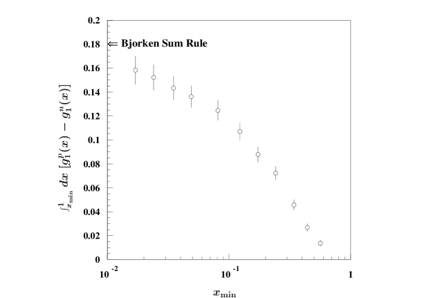
Figure 4: Difference between the measured proton (SLAC E-143) and neutron (SLAC E-154) integrals calculated from a minimum $x$ value, $x_{\rm min}$ up to $x$ of 1. The value is compared to the theoretical prediction from the Bjorken sum rule which makes a prediction over the full $x$ range. For the prediction, the Bjorken sum rule is evaluated up to third order in $\alpha_{s}$Larin et al. (1997) and at $Q^{2}$ = 5 (GeV/c)². Error bars on the data are dominated by systematic uncertainties and are highly correlated point-to-point. Figure from Abe et al. (1997).

Substituting the values of $g_{A}^{(3)}$ and $g_{A}^{(8)}$ from beta-decays (and assuming no subtraction constant correction) in the first moment equation (50) polarized deep inelastic data implies

$$g^{(0)}_{A}|_{\rm pDIS}=0.15-0.35$$ (59)

for the flavour singlet (Ellis Jaffe) moment corresponding to the polarized strangeness $\Delta s=-0.10\pm 0.04$ quoted in Section I. The measured value of $g^{(0)}_{A}|_{\rm pDIS}$ compares with the value 0.6 predicted by relativistic quark models and is less than 50% the value one would expect if strangeness were not important (viz. $g_{A}^{0}=g_{A}^{8}$) and the value predicted by relativistic quark models without additional gluonic input.

The small $x$ extrapolation of $g_{1}$ data is the largest source of experimental error on measurements of the nucleon’s axial charges from deep inelastic scattering. The first polarized deep inelastic experiments Ashman et al. (1988, 1989) used a simple Regge motivated extrapolation $\{g_{1}\sim{\tt constant}\}$ to evaluate the first moment sum-rules. More recent measurements quoted in the literature frequently use the technique of performing next-to-leading-order QCD motivated fits to the $g_{1}$ data, evolving the data points all to the same value of $Q^{2}$ and then extrapolating these fits to $x=0$. Values extracted from these fits using the “$\overline{\rm MS}$ scheme” include $g_{A}^{(0)}=0.23\pm 0.04\pm 0.06$ (SLAC experiment E155 at $Q^{2}=5$GeV² Anthony et al. (2000)), $g_{A}^{(0)}=0.19\pm 0.05\pm 0.04$ (SMC at $Q^{2}=1$GeV² Adeva et al. (1998b)), and $g_{A}^{(0)}=0.29\pm 0.10$ (the mean value at $Q^{2}=4$GeV² obtained in Blümlein and Böttcher (2002)).

Note that polarized deep inelastic scattering experiments measure $g_{1}$ between some small but finite value $x_{\rm min}$ and an upper value $x_{\rm max}$ which is close to one. As we decrease $x_{\rm min}\rightarrow 0$ we measure the first moment

$$\Gamma\equiv\lim_{x_{\rm min}\rightarrow 0}\ \int^{1}_{x_{\rm min}}dx\ g_{1}(x,Q^{2}).$$ (60)

Polarized deep inelastic experiments cannot, even in principle, measure at $x=0$ with finite $Q^{2}$. They miss any possible $\delta(x)$ terms which might exist in $g_{1}$ at large $Q^{2}$. That is, they miss any potential (leading twist) fixed pole correction to the deep inelastic spin sum rules.

Measurements of $g_{1}$ could be extended to smaller $x$ with a future polarized $ep$ collider. The low $x$ behaviour of $g_{1}$ is itself an interesting topic. Small $x$ measurements, besides reducing the error on the first moment (and gluon polarization, $\Delta g$, in the proton – see Section IX.E below), would provide valuable information about Regge and QCD dynamics at low $x$ where the shape of $g_{1}$ is particularly sensitive to the different theoretical inputs discussed in the literature: e.g. $(\alpha_{s}\ln^{2}{1\over x})^{k}$ resummation and DGLAP evolution Kwiecinski and Ziaja (1999), possible $Q^{2}$ independent Regge intercepts Cudell et al. (1999), and the non-perturbative “confinement physics” to hard (perturbative QCD) scale transition. Does the colour glass condensate of small $x$ physics Iancu et al. (2002) carry net spin polarization ? We refer to Ziaja Ziaja (2003) for a recent discussion of perturbative QCD predictions for the small $x$ behaviour of $g_{1}$ in deep inelastic scattering. In the conventional picture based on QCD evolution and no separate hard pomeron trajectory much larger changes in the effective intercepts which describe the shape of the structure functions at small Bjorken $x$ are expected in $g_{1}$ than in the unpolarized structure function $F_{2}$ so far studied at HERA as one increases $Q^{2}$ through the transition region from photoproduction to deep inelastic values of $Q^{2}$ Bass and De Roeck (2001). It will be fascinating to study this physics in future experiments, perhaps using a future polarized $ep$ collider.

III.3 $\nu p$ elastic scattering

Neutrino proton elastic scattering measures the proton’s weak axial charge $g_{A}^{\mbox{$\scriptscriptstyle(Z)$}}$ through elastic Z⁰ exchange. Because of anomaly cancellation in the Standard Model the weak neutral current couples to the combination $u-d+c-s+t-b$, viz.

$$J_{\mu 5}^{Z}\ =\ \mbox{\small${\displaystyle\frac{1}{2}}$}\biggl{\{}\,\sum_{q=u,c,t}-\sum_{q=d,s,b}\,\biggr{\}}\>\bar{q}\gamma_{\mu}\gamma_{5}q.$$ (61)

It measures the combination

$$2g_{A}^{\mbox{$\scriptscriptstyle(Z)$}}=\bigl{(}\Delta u-\Delta d-\Delta s\bigr{)}+\bigl{(}\Delta c-\Delta b+\Delta t\bigr{)}.$$ (62)

Heavy quark renormalization group arguments can be used to calculate the heavy $t$, $b$ and $c$ quark contributions to $g_{A}^{\mbox{$\scriptscriptstyle(Z)$}}$ both at leading-order Collins et al. (1978); Kaplan and Manohar (1988); Chetyrkin and Kühn (1993) and at next-to-leading-order (NLO) Bass et al. (2002). Working to NLO it is necessary to introduce “matching functions” Bass et al. (2003) to maintain renormalization group invariance through-out. The result is:

$$2g_{A}^{\mbox{$\scriptscriptstyle(Z)$}}=\bigl{(}\Delta u-\Delta d-\Delta s\bigr{)}_{\rm inv} + \hskip 0.56905pt{\cal H}\hskip 0.28453pt\bigl{(}\Delta u+\Delta d+\Delta s\bigr{)}_{\rm inv}$$

$$+ \ \ \ \ \ O(m_{t,b,c}^{-1})$$

where ${\cal H}$ is a polynomial in the running couplings $\widetilde{\alpha}_{h}$,

$${\cal H} = \mbox{\small${\displaystyle\frac{6}{23\pi}}$}\bigl{(}\widetilde{\alpha}_{b}-\widetilde{\alpha}_{t}\bigr{)}\Bigl{\{}1+\mbox{\small${\displaystyle\frac{125663}{82800\pi}}$}\widetilde{\alpha}_{b}+\mbox{\small${\displaystyle\frac{6167}{3312\pi}}$}\widetilde{\alpha}_{t}-\mbox{\small${\displaystyle\frac{22}{75\pi}}$}\widetilde{\alpha}_{c}\Bigr{\}}$$

$$\ \ \ \ \ \ \ -\mbox{\small${\displaystyle\frac{6}{27\pi}}$}\widetilde{\alpha}_{c}-\mbox{\small${\displaystyle\frac{181}{648\pi^{2}}}$}\widetilde{\alpha}_{c}^{2}+O\bigl{(}\widetilde{\alpha}_{t,b,c}^{3}\bigr{)}.$$

Here $(\Delta q)_{\rm inv}$ denotes the scale-invariant version of $\Delta q$ which are obtained from linear combinations of $g_{A}^{(3)}$, $g_{A}^{(8)}$ and $g_{A}^{(0)}|_{\rm pDIS}$ and $\widetilde{\alpha}_{h}$ denotes Witten’s renormalization-group-invariant running couplings for heavy quark physics Witten (1976). Taking $\widetilde{\alpha}_{t}=0.1$, $\widetilde{\alpha}_{b}=0.2$ and $\widetilde{\alpha}_{c}=0.35$ in (LABEL:eqc64), one finds a small heavy-quark correction factor ${\cal H}=-0.02$, with leading-order terms dominant. The factor $\bigl{(}\widetilde{\alpha}_{b}-\widetilde{\alpha}_{t}\bigr{)}$ ensures that all contributions from $b$ and $t$ quarks cancel for $m_{t}=m_{b}$ (as they should).

Modulo the small heavy-quark corrections quoted above, a precision measurement of $g_{A}^{(Z)}$, together with $g_{A}^{(3)}$ and $g_{A}^{(8)}$, would provide a weak interaction determination of $(\Delta s)_{\rm inv}$, complementary to the deep inelastic measurement of “$\Delta s$” in Eq.(6). The singlet axial charge in principle measurable in $\nu p$ elastic scattering is independent of any assumptions about the presence or absence of a subtraction at infinity correction to the Ellis-Jaffe deep inelastic first moment of $g_{1}$, the $x\sim 0$ behaviour of $g_{1}$ or SU(3) flavour breaking. Modulo any “subtraction at infinity” correction to the first moment of $g_{1}$, one obtains a rigorous sum-rule relating deep inelastic scattering in the Bjorken region of high-energy and high-momentum-transfer to three independent, low-energy measurements in weak interaction physics: the neutron and hyperon beta decays plus $\nu p$ elastic scattering.

A precision measurement of the $Z^{0}$ axial coupling to the proton is therefore of very high priority. Ideas are being discussed for a dedicated experiment Tayloe (2002). Key issues are the ability to measure close to the elastic point and a very low duty factor ($\sim 10^{-5}$) neutrino beam to control backgrounds, e.g. from cosmic rays.

The experiment E734 at BNL made the first attempt to measure $\Delta s$ in $\nu p$ and ${\overline{\nu}}p$ elastic scattering Ahrens et al. (1987). This experiment extracted differential cross-sctions $d\sigma/dQ^{2}$ in the range $0.4<Q^{2}<1.1$GeV². Extrapolating the axial form factor $(1-2\Delta s|_{\rm inv}/g_{A}^{(3)})/(1+Q^{2}/M_{A}^{2})^{2}$ to the elastic limit one obtains the value for $\Delta s$ Kaplan and Manohar (1988): $\Delta s=-0.15\pm 0.09$ taking the mass parameter in the dipole form factor to be $M_{A}=1.032\pm 0.036{\rm GeV}$. However, the data is also consistent with $\Delta s=0$ if one takes the mass parameter to be $M_{A}=1.06\pm 0.05{\rm GeV}$ which is consistent with the world average and therefore equally valid as a solution. That is, there is a strong correlation between the value of $\Delta s$ and the dipole mass parameter $M_{A}$ used in the analysis which prevents an unambiguous extraction of $\Delta s$ from the E734 data Garvey et al. (1993). A new dedicated precision experiment is required.

The neutral-current axial-charge $g_{A}^{(Z)}$ could also be measured through parity violation in light atoms Fortson and Lewis (1984); Khriplovich (1991); Missimer and Simons (1985); Bruss et al. (1998, 1999); Alberico et al. (2002); Campbell et al. (1989).

III.4 The Burkhardt-Cottingham sum rule

The Burkhardt-Cottingham sum rule Burkhardt and Cottingham (1970) reads:

$$\int_{Q^{2}/2M}^{\infty}d\nu G_{2}(Q^{2},\nu)={2M^{3}\over Q^{2}}\int_{0}^{1}dxg_{2}=0,\ \ \ \ \ \forall Q^{2}.$$ (65)

For deep inelastic scattering, this sum rule is derived by assuming that the moment formula (49) can be analytically continued to $n=0$. In general, the Burkhardt-Cottingham sum rule is derived by assuming no $\alpha\geq 0$ singularity in $G_{2}$ (or, equivalently, no ${1\over x}$ or more singular small behaviour in $g_{2}$) and no “subtraction at infinity” (from an $\alpha=J=0$ fixed pole in the real part of $G_{2}$) Jaffe (1990). The most precise measurements of $g_{2}$ to date in polarized deep inelastic scattering come from the SLAC E-155 and E-143 experiments, which report $\int_{0.02}^{0.8}dx\ g_{2}^{p}=-0.042\pm 0.008$ for the proton and $\int_{0.02}^{0.8}dx\ g_{2}^{d}=-0.006\pm 0.011$ for the deuteron at $Q^{2}=5$GeV² Anthony et al. (2003). New, even more accurate, measurements of $g_{2}$ (for the neutron using a ³He target) from Jefferson Laboratory Amarian et al. (2004) for $Q^{2}$ between 0.1 and 0.9 GeV² are consistent with the sum rule. Further measurements to test the Burkhardt-Cottingham sum rule would be most valuable, particularly given the SLAC proton result quoted above.

Figure 5: The $Q^{2}$ averaged measured of $xg_{2}$ (SLAC data) compared with the twist-two Wandzura-Wilczek contribution $g_{2}^{WW}$ term (solid line) and several quark model calculations. Figure from Anthony et al. (2003).

The formula (49) indicates that $g_{2}$ can be written as the sum

$$g_{2}=g_{2}^{\rm WW}(x)+{\overline{g}}_{2}(x)$$ (66)

of a twist-two term Wandzura and Wilczek (1977), denoted $g_{2}^{\rm WW}$

$$g_{2}^{\rm WW}=-g_{1}(x)+\int_{x}^{1}{dy\over y}g_{1}(y)$$ (67)

and a second contribution ${\bar{g}}_{2}$ which is the sum of a higher-twist (twist 3) contribution $\xi(x,Q^{2})$ and a “transversity” term $h_{1}(x,Q^{2})$ which is suppressed by the ratio of the quark to target nucleon masses and therefore negligible for light $u$ and $d$ quarks

$${\overline{g}}_{2}(x,Q^{2})=-\int_{x}^{1}{dy\over y}{\partial\over\partial y}\biggl{(}{m_{q}\over M}h_{1}(y,Q^{2})+\xi(y,Q^{2})\biggr{)}$$ (68)

– see Cortes et al. (1992). The first moment of the twist 2 contribution $g_{2}^{\rm WW}$ vanishes through integrating the convolution formula (67). If one drops the transversity contribution from the formalism (being proportional to the light quark mass), one obtains the equation

$${\tilde{d}}_{2}(Q^{2})=3\int_{0}^{1}dxx^{2}\biggl{[}g_{2}(x,Q^{2})-g_{2}^{\rm WW}(x,Q^{2})\biggr{]}$$ (69)

for the leading twist 3 matrix element in Eq.(49). The values extracted from dedicated SLAC measurements are $d_{2}^{p}=0.0032\pm 0.0017$ for the proton and $d_{2}^{n}=0.0079\pm 0.0048$ for the neutron – that is, consistent with zero (no twist-3) at two standard deviations Anthony et al. (2003). These twist 3 matrix elements are related in part to the response of the collective colour electric and magnetic fields to the spin of the nucleon. Recent analyses attempt to extract the twist-four corrections to $g_{1}$. The results and the gluon field polarizabilities are small and consistent with zero Deur et al. (2004).

III.5 The Gerasimov-Drell-Hearn sum rule

The Gerasimov-Drell-Hearn (GDH) sum-rule Gerasimov (1965); Drell and Hearn (1966) for spin dependent photoproduction relates the difference of the two cross-sections for the absorption of a real photon with spin polarized anti-parallel, $\sigma_{1\over 2}$, and parallel, $\sigma_{3\over 2}$ , to the target spin to the square of the anomalous magnetic moment of the target. The GDH sum rule reads:

$$\int_{\rm threshold}^{\infty}{d\nu\over\nu}(\sigma_{1\over 2}-\sigma_{3\over 2}) = {8\pi^{2}\alpha\over M^{2}}\int_{\rm threshold}^{\infty}{d\nu\over\nu}G_{1}$$ (70)

$$= -{2\pi^{2}\alpha\over M^{2}}\kappa^{2}$$

where $\kappa$ is the anomalous magnetic moment. The sum rule follows from the very general principles of causality, unitarity, Lorentz and electromagnetic gauge invariance and one assumption: that the $g_{1}$ spin structure function satisfies an unsubtracted dispersion relation. Modulo the no-subtraction hypothesis, the Gerasimov-Drell-Hearn sum-rule is valid for a target of arbitrary spin $S$, whether elementary or composite Brodsky and Primack (1969) – for reviews see Bass (1997) and Drechsel and Tiator (2004).

Figure 6: The spin dependent photoproduction cross-section for the proton target (ELSA and MAMI data). Figure courtesy of K. Helbing.

Figure 7: Running GDH integral for the proton (ELSA and MAMI). Figure courtesy of K. Helbing.

The GDH sum-rule is derived by setting $\nu=0$ in the dispersion relation for $A_{1}$, Eq.(LABEL:eqc38). For small photon energy $\nu\rightarrow 0$

$$A_{1}(0,\nu)=-{1\over 2}\kappa^{2}+{\tilde{\gamma}}\nu^{2}+O(\nu^{4}).$$ (71)

Here $\gamma_{N}={\alpha\over M^{2}}{\tilde{\gamma}}$ is the spin polarizability which measures the stiffness of the nucleon spin against electromagnetic induced deformations relative to the axis defined by the nucleon’s spin. This low-energy theorem follows from Lorentz invariance and electromagnetic gauge invariance (plus the existence of a finite mass gap between the ground state and continuum contributions to forward Compton scattering) Brodsky and Primack (1969); Low (1954); Gell-Mann and Goldberger (1954).

The integral in Eq.(70) converges for each of the leading Regge contributions (discussed in Section II.B). If the sum rule were observed to fail (with a finite integral) the interpretation would be a “subtraction at infinity” induced by a $J=1$ fixed pole in the real part of the spin amplitude $A_{1}$ Abarbanel and Goldberger (1968).

Present experiments at ELSA and MAMI are aimed at measuring the GDH integrand through the range of incident photon energies $E_{\gamma}=$ 0.14 - 0.8 GeV (MAMI) Ahrens et al. (2000, 2001, 2002) and 0.7 - 3.1 GeV (ELSA) Dutz et al. (2003). The inclusive cross-section for the proton target ${\sigma_{3\over 2}-\sigma_{1\over 2}}$ is shown in Fig. 6. The presently analysed GDH integral on the proton is shown in Fig. 7 and is dominated by the $\Delta$ resonance contribution. (The contribution to the sum-rule from the unmeasured region close to threshold is estimated from the MAID model Drechsel et al. (2003).) The combined data from the ELSA-MAMI experiments suggest that the contribution to the GDH integral for a proton target from energies $\nu<3$GeV exceeds the total sum rule prediction (-204.5$\mu$b) by about 5-10% Helbing (2002). Phenomenological estimates suggest that about $+25\pm 10\mu$b of the sum rule may reside at higher energies Bass and Brisudova (1999); Bianchi and Thomas (1999) and that this high energy contribution is predominantly in the isovector channel. (It should be noted, however, that any 10% fixed pole correction would be competitive with this high energy contribution within the errors.) Further measurements, including at higher energy, would be valuable. Preliminary data on the neutron has just been released from MAMI and ELSA Helbing (2004). This data, if confirmed, suggests that the neutron GDH integal, if it indeed obeys the GDH sum-rule, will require a large (mainly isovector) contribution (perhaps 45$\mu$b) from photon energies $E_{\gamma}$ greater than about 1800 MeV. With the caution that these data are still preliminary, it is interesting to note that, just like the measured $g_{1}$ at deep inelastic $Q^{2}$, the high-energy part of the spin dependent cross-section $\sigma_{1\over 2}-\sigma_{3\over 2}$ at $Q^{2}=0$ seems to be largely isovector prompting the question whether there is some physics conspiracy to suppress the singlet term. It should be noted however that perturbative QCD motivated fits to $g_{1}$ data with a positive polarized gluon distribution (and no node in it) predict that $g_{1}$ should develop a strong negative contribution at $x<0.0001$ at deep inelastic $Q^{2}$ – see e.g. De Roeck et al. (1999) and references therein.

In addition to the GDH sum-rule, one also finds a second sum-rule for the nucleon’s spin polarizability. This spin polarizability sum-rule is derived by taking the second derivative of $A_{1}(Q^{2},\nu)$ in the dispersion relation (LABEL:eqc38) and evaluating the resulting expression at $\nu=0$, viz. ${\partial^{2}\over\partial\nu^{2}}A_{1}(Q^{2},\nu)|_{\nu=0}$. One finds

$$\int_{0}^{\infty}{d\nu^{\prime}\over\nu^{\prime 3}}\Biggl{(}\sigma_{1\over 2}-\sigma_{3\over 2}\Biggr{)}(\nu^{\prime})={4\pi^{2}}\ \gamma_{N}.$$ (72)

In comparison with the GDH sum-rule the relevant information is now concentrated more on the low energy side because of the $1/\nu^{\prime 3}$ weighting factor under the integral. Main contributions come from the $\Delta$(1232) resonance and the low energy pion photoproduction continuum described by the electric dipole amplitude $E_{0+}$. The value extracted from MAMI data Drechsel et al. (2003)

$$\gamma_{p}=(-1.01\pm 0.13).10^{-4}\ {\rm fm}^{4}$$ (73)

is within the range of predictions of chiral perturbation theory.

Further experiments to test the GDH sum-rule and to measure the $\sigma_{1\over 2}-\sigma_{3\over 2}$ at and close to $Q^{2}=0$ are being carried out at Jefferson Laboratory, GRAAL at Grenoble, LEGS at BNL, and SPRING-8 in Japan.

We note two interesting properties of the GDH sum rule.

First, we write the anomalous magnetic moment $\kappa$ as the sum of its isovector $\kappa_{V}$ and isoscalar $\kappa_{S}$ contributions, viz. $\kappa_{N}=\kappa_{S}+\tau_{3}\kappa_{V}.$ One then obtains the isospin dependent expressions:

$$({\rm GDH})_{I=0}=({\rm GDH})_{VV}+({\rm GDH})_{SS} = -{2\pi^{2}\alpha\over m^{2}}(\kappa_{V}^{2}+\kappa_{S}^{2})$$

$$({\rm GDH})_{I=1}=({\rm GDH})_{VS} = -{2\pi^{2}\alpha\over m^{2}}2\kappa_{V}\kappa_{S}.$$

The physical values of the proton and nucleon anomalous magnetic moments $\kappa_{p}=1.79$ and $\kappa_{n}=-1.91$ correspond to $\kappa_{S}=-0.06$ and $\kappa_{V}=+1.85$. Since $\kappa_{S}/\kappa_{V}\simeq-{1\over 30}$, it follows that $({\rm GDH})_{SS}$ is negligible compared to $({\rm GDH})_{VV}$. That is, to good approximation, the isoscalar sum-rule $({\rm GDH})_{I=0}$ measures the isovector anomalous magnetic moment $\kappa_{V}$. Given this isoscalar measurement, the isovector sum-rule $({\rm GDH})_{I=1}$ then measures the isoscalar anomalous magnetic moment $\kappa_{S}$.

Second, the anomalous magnetic moment is measured in the matrix element of the vector current. Furry’s theorem tells us that the real-photon GDH integral for a gluon or a photon target vanishes. Indeed, this is the reason that the first moment of the $g_{1}$ spin structure function for a real polarized photon target vanishes to all orders and at every twist: $\int_{0}^{1}dx\ g_{1}^{\gamma}(x,Q^{2})$ independent of the virtuality $Q^{2}$ of the second photon that it is probed with Bass et al. (1998). Assuming correction to the GDH sum rule, this result implies that the two non-perturbative gluon exchange contribution to $\sigma_{1\over 2}-\sigma_{3\over 2}$ which behaves as $\ln\nu/\nu$ in the high energy Regge limit has a node at some value $\nu=\nu_{0}$ so that it does not contribute to the GDH integral. There is no axial anomaly contribution to the anomalous magnetic moment and hence no axial anomaly contribution to the GDH sum-rule.

III.6 The transition region

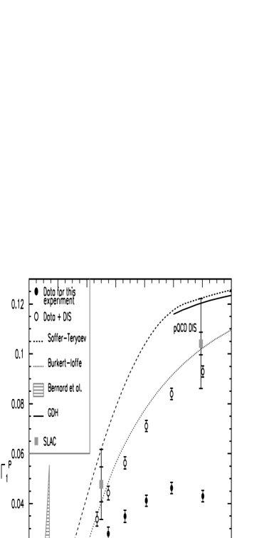
Figure 8: Data from JLab (CLAS) and SLAC on the low $Q^{2}$ behaviour of $\int_{0}^{1}dxg_{1}^{p}$ compared to various theoretical models interpolating the scaling and photoproduction limits Fatemi et al. (2003).

Several experiments have explored the transition region between polarized photoproduction (the physics of the GDH sum-rule) and polarized deep inelastic scattering (the physics of the Bjorken sum-rule and $g_{A}^{(0)}$ through the Ellis-Jaffe moment).

The $Q^{2}$ dependent quantity Anselmino et al. (1989)

$$\Gamma(Q^{2})\equiv I(Q^{2}) = \int_{{Q^{2}\over 2M}}^{\infty}{d\nu\over\nu}G_{1}(\nu,Q^{2})$$ (75)

$$= {2M^{2}\over Q^{2}}\int_{0}^{1}dxg_{1}(x,Q^{2})$$

interpolates between the two limits with $I(0)=-{1\over 4}\kappa^{2}_{N}$ implied by the GDH sum rule. Measurements of $\int_{0}^{1}dxg_{1}^{p}={Q^{2}\over 2M^{2}}I(Q^{2})$ are shown in Fig. 8. Note the negative slope predicted at $Q^{2}=0$ by the GDH sum rule and the sign change around $Q^{2}\sim 0.3$GeV². The shape of the curve is driven predominantly by the role of the $\Delta$ resonance and the $1/Q^{2}$ pole in Eq.(75). Fig. 8 shows also the predictions of various models Soffer and Teryaev (1993); Burkert and Ioffe (1994) which try to describe the intermediate $Q^{2}$ range through a combination of resonance physics and vector-meson dominance at low $Q^{2}$ and scaling parton physics at DIS $Q^{2}$. Chiral perturbation theory Bernard et al. (2003) may describe the behaviour of this “generalized GDH integral” close to threshold – see the shaded band in Fig. 8.

In the model of Ioffe and collaborators Anselmino et al. (1989); Burkert and Ioffe (1994) the integral at low to intermediate $Q^{2}$ for the inelastic part of $(\sigma_{A}-\sigma_{P})$ is given as the sum of a contribution from resonance production, denoted $I^{\rm res}(Q^{2})$, which has a strong $Q^{2}$ dependence for small $Q^{2}$ and then drops rapidly with $Q^{2}$, and a non-resonant vector-meson dominance contribution which they took as the sum of a monopole and a dipole term, viz.

$$I(Q^{2})=I^{\rm res}(Q^{2})+2M^{2}\Gamma^{\rm as}\Biggl{(}{1\over Q^{2}+\mu^{2}}-{C\mu^{2}\over(Q^{2}+\mu^{2})^{2}}\Biggr{)}.$$ (76)

Here $\Gamma^{\rm as}$ is taken as

$$\Gamma^{\rm as}=\int_{0}^{1}dxg_{1}(x,\infty)$$ (77)

and

$$C=1+{1\over 2}\ {\mu^{2}\over M^{2}}\ {1\over\Gamma^{\rm as}}\ \Bigl{(}{1\over 4}\kappa^{2}+I^{\rm res}(0)\Bigr{)}.$$ (78)

The mass parameter $\mu$ is identified with rho meson mass, $\mu^{2}\simeq m_{\rho}^{2}$.

IV PARTONS AND SPIN STRUCTURE FUNCTIONS

IV.1 The QCD parton model

We now return to $g_{1}$ in the scaling regime of polarized deep inelastic scattering. As noted in Section II.A above, in the (pre-QCD) parton model $g_{1}$ is written as

$$g_{1}(x)={1\over 2}\sum_{q}e_{q}^{2}\Delta q(x)$$ (79)

where $e_{q}$ denotes the quark charge and $\Delta q(x)$ is the polarized quark distribution.

In QCD we have to consider the effects of gluon radiation and (renormalization group) mixing of the flavour-singlet quark distribution with the polarized gluon distribution of the proton. The parton model description of polarized deep inelastic scattering involves writing the deep inelastic structure functions as the sum over the convolution of “soft” quark and gluon parton distributions with “hard” photon-parton scattering coefficients:

$$g_{1}(x) = \Biggl{\{}{1\over 12}(\Delta u-\Delta d)+{1\over 36}(\Delta u+\Delta d-2\Delta s)\Biggr{\}}\otimes C^{q}_{ns}$$

$$+{1\over 9}\Biggl{\{}(\Delta u+\Delta d+\Delta s)\otimes C^{q}_{s}+f\Delta g\otimes C^{g}\Biggr{\}}.$$

Here $\Delta q(x)$ and $\Delta g(x)$ denote the polarized quark and gluon parton distributions, $C^{q}(z)$ and $C^{g}(z)$ denote the corresponding hard scattering coefficients, and $f$ is the number of quark flavours liberated into the final state ($f=3$ below the charm production threshold). The parton distributions contain all the target dependent information and describe a flux of quark and gluon partons into the (target independent) interaction between the hard photon and the parton which is described by the coefficients and which is calculable using perturbative QCD. The perturbative coefficients are independent of infra-red mass singularities in the photon-parton collision which are absorbed into the soft parton distributions (and softened by confinement related physics).

The separation of $g_{1}$ into “hard” and “soft” is not unique and depends on the choice of “factorization scheme”. For example, one might use a kinematic cut-off on the partons’ transverse momentum squared ($k_{t}^{2}>\lambda^{2}$) to define the factorization scheme and thus separate the hard and soft parts of the phase space for the photon-parton collision. The cut-off $\lambda^{2}$ is called the factorization scale. The coefficients have the perturbative expansion $C^{q}=\delta(1-x)+{\alpha_{s}\over 2\pi}f^{q}(x,{Q^{2}/\lambda^{2}})$ and $C^{g}={\alpha_{s}\over 2\pi}f^{g}(x,{Q^{2}/\lambda^{2}})$ where the strongest singularities in the functions $f^{q}$ and $f^{g}$ as $x\rightarrow 1$ are $\ln(1-x)/(1-x)_{+}$ and $\ln(1-x)$ respectively – see e.g. Lampe and Reya (2000). The deep inelastic structure functions are dependent on $Q^{2}$ and independent of the factorization scale $\lambda^{2}$ and the “scheme” used to separate the $\gamma^{*}$-parton cross-section into “hard” and “soft” contributions. Examples of different “schemes” one might use include using modified minimal subtraction (${\rm\overline{MS}}$) ’t Hooft and Veltman (1972); Bodwin and Qiu (1990) to regulate the mass singularities which arise in scattering from massless partons, and cut-offs on other kinematic variables such as the invariant mass squared or the virtuality of the struck quark. Other schemes which have been widely used in the literature and analysis of polarized deep inelastic scattering data are the “AB” Ball et al. (1996) and “CI” (chiral invariant) Cheng (1996) or “JET” Leader et al. (1998) schemes. We illustrate factorization scheme dependence and the use of these schemes in the analysis of $g_{1}$ data in Sections VI.D and IX.C below.

If the same “scheme” is applied consistently to all hard processes then the factorization theorem asserts that the parton distributions that one extracts from experiments should be process independent Collins (1993a). In other words, the same polarized quark and gluon distributions should be obtained from future experiments involving polarized hard QCD processes in polarized proton proton collisions (e.g. at RHIC) and polarized deep inelastic scattering experiments. The factorization theorem for unpolarized hard processes has been successfully tested in a large number of experiments involving different reactions at various laboratories. Tests of the polarized version await future independent measurements of the polarized gluon and sea-quark distributions from a variety of different hard scattering processes with polarized beams.

IV.2 Light-cone correlation functions

The (spin-dependent) parton distributions may also be defined via the operator product expansion. For $g_{1}$ this means that the odd moments of the polarized quark and gluon distributions project out the target matrix elements of the renormalized, spin-odd, composite operators which appear in the operator product expansion, viz.

$$2Ms_{+}(p_{+})^{2n}\int^{1}_{0}dx\ x^{2n}\Delta q(x,\mu^{2})$$

$$\ \ \ \ \ \ \ \ =\langle p,s|\biggl{[}{\overline{q}}(0)\gamma_{+}\gamma_{5}(iD_{+})^{2n}q(0)\biggr{]}_{\mu^{2}}|p,s\rangle$$

(81)

$$2Ms_{+}(p_{+})^{2n}\int^{1}_{0}dx\ x^{2n}\Delta g(x,\mu^{2})$$

$$\ \ \ \ \ \ \ \ =\langle p,s|\biggl{[}{\bf\rm Tr}\ G_{+\alpha}(0)(iD_{+})^{2n-1}{\tilde{G}}^{\alpha}_{\ +}(0)\biggr{]}_{\mu^{2}}|p,s\rangle$$

$$\ \ \ \ \ \ \ \ \ \ \ \ \ \ \ \ \ \ \ \ \ \ \ \ \ \ \ \ \ \ \ \ \ \ \ \ \ \ \ \ \ \ (n\geq 1).$$

(82)

The association of $\Delta q(x,\mu^{2})$ with quarks and $\Delta g(x,\mu^{2})$ with gluons follows when we evaluate the target matrix elements in Eqs.(81) and (82) in the light-cone gauge, where $D_{+}\rightarrow\partial_{+}$ and the explicit dependence of $D_{+}$ on the gluon field drops out. The operator product expansion involves writing the product of electromagnetic currents $J_{\mu}(z)J_{\nu}(0)$ in Eq.(11) as the expansion over gauge invariantly renormalized, local, composite quark and gluonic operators at lightlike separation $z^{2}\rightarrow 0$ – the realm of deep inelastic scattering Muta (1998). The subscript $\mu^{2}$ on the operators in Eq.(82) emphasises the dependence on the renormalization scale.

Mathematically, the relation between the parton distributions and the operator product expansion is given in terms of light-cone correlation functions of point split operator matrix elements along the light-cone. Define

$$\psi^{\pm}=P^{\pm}\psi$$ (83)

where

$$P^{\pm}={1\over 2}(1\pm\alpha_{3})={1\over 2}\gamma^{\pm}\gamma^{\mp}.$$ (84)

The polarized quark and antiquark distributions are given by

$$\Delta\psi(x) = {1\over 2\sqrt{2}\pi}\int d\xi^{-}e^{-ixM\xi^{-}/\sqrt{2}}$$

$$\langle p,s|(\psi^{+R})^{\dagger}(\xi^{-})\psi^{+R}(0)$$

$$\ \ \ \ \ \ \ \ \ \ \ \ \ \ -(\psi^{+L})^{\dagger}(\xi^{-})\psi^{+L}(0)|p,s\rangle,$$

$$\Delta{\bar{\psi}}(x) = {1\over 2\sqrt{2}\pi}\int d\xi^{-}e^{-ixM\xi^{-}/\sqrt{2}}$$

$$\langle p,s|\psi^{+L}(\xi^{-})(\psi^{+L})^{\dagger}(0)$$

$$\ \ \ \ \ \ \ \ \ \ \ \ \ \ -\psi^{+R}(\xi^{-})(\psi^{+R})^{\dagger}(0)|p,s\rangle.$$

In this notation $\Delta q=\Delta\psi+\Delta{\bar{\psi}}$. The non-local operator in the correlation function is rendered gauge invariant through a path ordered exponential which simplifies to unity in the light-cone gauge $A_{+}=0$. Taking the moments of these distributions reproduces the results of the operator product expansion in Eq. (48). The light-cone correlation function for the polarized gluon distribution is

$$x\Delta g(x) = {i\over 2\sqrt{2}M\pi}\int d\xi^{-}\ e^{-ix\xi^{-}M/\sqrt{2}}$$

$$\langle p,s|G_{+\nu}(\xi^{-}){\tilde{G}}_{\ +}^{\nu}(0)-G_{+\nu}(0){\tilde{G}}_{\ +}^{\nu}(\xi^{-})|p,s\rangle.$$

In the light-cone gauge ($A_{+}=0$) one finds $G^{+\nu}_{a}=\partial^{+}A^{\nu}_{a}-\partial^{\nu}A^{+}_{a}=\partial^{+}A^{\nu}_{a}$ so that

$$G^{+\nu}{\tilde{G}}_{\nu}^{\ +}=G^{+}_{R}G_{-L}-G^{+}_{L}G_{-R}=G^{+}_{R}G^{+R}-G^{+}_{L}G^{+L}.$$ (88)

Thus $\Delta g(x)$ measures the distribution of gluon polarization in the nucleon. One can evaluate the first moment of $\Delta g(x)$ from its light-cone correlation function. One first assumes that

$$\lim_{x\rightarrow 0^{+}}x\Delta g(x)=0.$$ (89)

In $A_{+}=0$ gauge the first moment becomes

$$\int_{0}^{1}dx\Delta g(x)=$$

$${1\over\sqrt{2}M}\biggl{[}\langle A^{\nu}(\xi^{-}){\tilde{G}}^{\ +}_{\nu}(0)\rangle|_{\xi^{-}\rightarrow\infty}-\langle A^{\nu}(0){\tilde{G}}^{\ +}_{\nu}(0)\rangle\biggr{]}$$

(90)

– that is, the sum of the forward matrix element of the gluonic Chern Simons current $K_{+}$ plus a surface term Manohar (1990) which may or may not vanish in QCD.

V FIXED POLES

Fixed poles are exchanges in Regge phenomenology with no $t$ dependence: the trajectories are described by $J=\alpha(t)=0$ or 1 for all $t$ Abarbanel et al. (1967); Brodsky et al. (1972); Landshoff and Polkinghorne (1972). For example, for fixed $Q^{2}$ a $t-$independent real constant term in the spin amplitude $A_{1}$ would correspond to a $J=1$ fixed pole. Fixed poles are excluded in hadron-hadron scattering by unitarity but are not excluded from Compton amplitudes (or parton distribution functions) because these are calculated only to lowest order in the current-hadron coupling. Indeed, there are two famous examples where fixed poles are required: (by current algebra) in the Adler sum rule for W-boson nucleon scattering, and to reproduce the Schwinger term sum rule for the longitudinal structure function measured in unpolarized deep inelastic $ep$ scattering. We review the derivation of these fixed pole contributions, and then discuss potential fixed pole corrections to the Burkhardt-Cottingham, $g_{1}$ and Gerasimov-Drell-Hearn sum-rules. Fixed poles in the real part of the forward Compton amplitude have the potential to induce “subtraction at infinity” corrections to sum rules for photon nucleon (or lepton nucleon) scattering. For example, a $\nu$ independent term in the real part of $A_{1}$ would induce a subtraction constant correction to the spin sum rule for the first moment of $g_{1}$. Bjorken scaling at large $Q^{2}$ constrains the $Q^{2}$ dependence of the residue of any fixed pole in the real of the forward Compton amplitude (e.g. $\beta_{1}(Q^{2})$ and $\beta_{2}(Q^{2})$ in the dispersion relations (LABEL:eqc41) ). To be consistent with scaling these residues must decay as or faster than $1/Q^{2}$ as $Q^{2}\to\infty$. That is, they must be nonpolynomial in $Q^{2}$.

V.1 Adler sum rule

The first example we consider is the Adler sum rule for W-boson nucleon scattering Adler (1966):

$$\int_{Q^{2}/2M}^{+\infty}d\nu\biggl{[}W_{2}^{\bar{\nu}p}(\nu,Q^{2})-W_{2}^{\nu p}(\nu,Q^{2})\biggr{]}$$

$$\ \ \ \ \ =\int_{0}^{1}{dx\over x}\biggl{[}F_{2}^{\bar{\nu}p}(x,Q^{2})-F_{2}^{\nu p}(x,Q^{2})\biggr{]}$$

$$\ \ \ \ \ =\begin{array}[]{c}4-2\cos^{2}\theta_{c}\ \ \ \ \ ({\rm BCT})\\ 2\ \ \ \ \ \ \ \ \ \ \ \ \ \ \ \ \ \ \ ({\rm ACT}).\end{array}$$ (93)

Here $\theta_{c}$ is the Cabibbo angle, and BCT and ACT refer to below and above the charm production threshold.

The Adler sum rule is derived from current algebra. The right hand side of the sum rule is the coefficient of a $J=1$ fixed pole term

$${i\over\pi}f_{abc}\ F_{c}\ \biggl{[}(p_{\mu}q_{\nu}+q_{\mu}p_{\nu})-M\nu g_{\mu\nu}\biggr{]}/Q^{2}$$ (94)

in the imaginary part of the forward Compton amplitude for W-boson nucleon scattering Heimann et al. (1972). This fixed pole term is required by the commutation relations between the charge raising and lowering weak currents

$$q_{\mu}T^{\mu\nu}_{ab} = -{1\over\pi}\int d^{4}x\ e^{iq.x}\ \langle p,s|\biggl{[}J_{a}^{0}(x),J^{\nu}_{b}(0)\biggr{]}|p,s\rangle\delta(x^{0})$$ (95)

$$= -{i\over\pi}f_{abc}\langle ps|J_{c}^{\nu}(0)|ps\rangle.$$

Here $F_{c}$ is a generalized form factor at zero momentum transfer:

$$\langle p,s|J_{c}^{\nu}(0)|p,s\rangle\equiv p^{\nu}F_{c}.$$ (96)

The fixed pole term appears in lowest order perturbation theory, and is not renormalized because it is a consequence of the charge algebra. The Adler sum rule is protected against radiative QCD corrections

V.2 Schwinger term sum rule

Our second example is the Schwinger term sum rule Broadhurst et al. (1973) which relates the logarithmic integral in $\omega$ (or Bjorken $x$) of the longitudinal structure function $F_{L}(\omega,Q^{2})$ ($F_{L}={1\over 2}\omega F_{2}-F_{1}$) measured in unpolarized deep inelastic scattering to the target matrix element of the operator Schwinger term ${\cal S}$ defined through the equal-time commutator of the electromagnetic charge and current densities

$$\langle p,s|\biggl{[}J_{0}({\vec{y}},0),J_{i}(0)\biggr{]}|p,s\rangle=i\ \partial_{i}\ \delta^{3}({\vec{y}})\ {\cal S}.$$ (97)

The Schwinger term sum rule reads

$${\cal S}=\lim_{Q^{2}\rightarrow\infty}\biggl{[}4\int_{1}^{\infty}{d\omega\over\omega}{\tilde{F}}_{L}(\omega,Q^{2})-4\sum_{\alpha>0}\gamma(\alpha,Q^{2})/\alpha-C(q^{2})\biggr{]}.$$ (98)

Here $C(Q^{2})$ is the nonpolynomial residue of any $J=0$ fixed pole contribution in the real part of $T_{2}$ and

$${\tilde{F}}_{L}(\omega,Q^{2})=F_{L}(\omega,Q^{2})-\sum_{\alpha\geq 0}\gamma(\alpha,Q^{2})\omega^{\alpha}$$ (99)

represents $F_{L}$ with the leading ($\alpha>0$) Regge behaviour subtracted. The integral in Eq.(98) is convergent because ${\tilde{F}}_{L}(\omega,Q^{2})$ is defined with all Regge contributions with effective intercept greater than or equal to zero removed from $F_{L}(Q^{2},\omega)$. The Schwinger term ${\cal S}$ vanishes in vector gauge theories like QCD.

Since $F_{L}(\omega,Q^{2})$ is positive definite, it follows that QCD possesses the required non-vanishing $J=0$ fixed pole in the real part of $T_{2}$.

V.3 Burkhardt-Cottingham sum rule

The third example, and the first in connection with spin, is the Burkhardt-Cottingham sum rule for the first moment of $g_{2}$ Burkhardt and Cottingham (1970):

$$\int_{Q^{2}/2M}^{\infty}d\nu\ G_{2}(Q^{2},\nu)={2M^{3}\over Q^{2}}\int_{0}^{1}dxg_{2}=0.$$

Suppose that future experiments find that the sum rule is violated and that the integral is finite. The conclusion Jaffe (1990) would be a $J=0$ fixed pole with nonpolynomial residue in the real part of $A_{2}$. To see this work at fixed $Q^{2}$ and assume that all Regge-like singularities contributing to $A_{2}(\nu,Q^{2})$ have intercept less than zero so that

$$A_{2}(\nu,Q^{2})\sim\nu^{-1-\epsilon}$$ (100)

as $\nu\rightarrow\infty$ for some $\epsilon>0$. Then the large $\nu$ behaviour of $A_{2}$ is obtained by taking $\nu\rightarrow\infty$ under the $\nu^{\prime}$ integral giving

$$A_{2}(Q^{2},\nu)\sim-{2\over\pi\nu}\int_{Q^{2}/2M}^{\infty}d\nu^{\prime}\ {\rm Im}A_{2}(Q^{2},\nu^{\prime})$$ (101)

which contradicts the assumed behaviour unless the integral vanishes; hence the sum rule. If there is an $\alpha(0)=0$ fixed pole in the real part of $A_{2}$ the fixed pole will not contribute to ${\rm Im}A_{2}$ and therefore not spoil the convergence of the integral.

One finds

$$\beta_{2}(Q^{2})\sim-{2\over\pi M}\int_{Q^{2}/2M}^{\infty}d\nu^{\prime}\ {\rm Im}A_{2}(Q^{2},\nu^{\prime})$$ (102)

for the residue of any $J=0$ fixed pole coupling to $A_{2}(Q^{2},\nu)$.

V.4 $g_{1}$ spin sum rules

Scaling requires that any fixed pole correction to the Ellis-Jaffe $g_{1}$ sum rule must have nonpolynomial residue. Through Eq.(LABEL:eqc41), the fixed pole coefficient $\beta_{1}(Q^{2})$ must decay as or faster than $O(1/Q^{2})$ as $Q^{2}\rightarrow\infty$. The coefficient is further constrained by the requirement that $G_{1}$ contains no kinematic singularities (for example at $Q^{2}=0$). In Section VI.C we will identify a potential leading-twist topological $x=0$ contribution to the first moment of $g_{1}$ through analysis of the axial anomaly contribution to $g_{A}^{(0)}$. This zero-mode topological contribution (if finite) generates a leading twist fixed pole correction to the flavour-singlet part of $\int_{0}^{1}dxg_{1}$. If present, this fixed pole will also violate the Gerasimov-Drell-Hearn sum rule (since the two sum rules are derived from $A_{1}$) unless the underlying dynamics suppress the fixed pole’s residue at $Q^{2}=0$. The possibility of a fixed pole correction to $g_{1}$ spin sum-rules was raised in pre-QCD work as early as Abarbanel and Goldberger (1968) and Heimann (1973).

Note that any fixed pole correction to the Gerasimov-Drell-Hearn sum rule is most probably a non-perturbative effect. The sum rule (LABEL:eqc41) has been verified to $O(\alpha^{2})$ for all $2\rightarrow 2$ processes $\gamma a\rightarrow bc$ where $a$ is either a real lepton, quark, gluon or elementary Higgs target Altarelli et al. (1972); Brodsky and Schmidt (1995), and for electrons in QED to $O(\alpha^{3})$ Dicus and Vega (2001).

One could test for a fixed pole correction to the Ellis-Jaffe moment through a precision measurement of the flavour singlet axial charge from an independent process where one is not sensitive to theoretical assumptions about the presence or absence of a $J=1$ fixed pole in $A_{1}$. Here the natural choice is elastic neutrino proton scattering where the parity violating part of the cross-section includes a direct weak interaction measurement of the scale invariant flavour-singlet axial charge $g_{A}^{(0)}|_{\rm inv}$.

A further test could come from a precision measurement of the $Q^{2}$ dependence of the polarized gluon distribution at next-to-next-to-leading order accuracy where one becomes sensitive to any possible leading-twist subtraction constant – see below Eq.(129).

The subtraction constant fixed pole correction hypothesis could also, in principle, be tested through measurement of the real part of the spin dependent part of the forward deeply virtual Compton amplitude. While this measurement may seem extremely difficult at the present time one should not forget that Bjorken believed when writing his original Bjorken sum rule paper that the sum rule would never be tested!

VI THE AXIAL ANOMALY, GLUON TOPOLOGY AND THE FLAVOUR SINGLET AXIAL CHARGE $g_{A}^{(0)}$

We next discuss the role of the axial anomaly in the interpretation of $g_{A}^{(0)}$.

VI.1 The axial anomaly

In QCD one has to consider the effects of renormalization. The flavour singlet axial vector current $J_{\mu 5}^{GI}$ in Eq.(53) satisfies the anomalous divergence equation Adler (1969); Bell and Jackiw (1969); Crewther (1978)

$$\partial^{\mu}J^{GI}_{\mu 5}=2f\partial^{\mu}K_{\mu}+\sum_{i=1}^{f}2im_{i}\bar{q}_{i}\gamma_{5}q_{i}$$ (103)

where

$$K_{\mu}={g^{2}\over 32\pi^{2}}\epsilon_{\mu\nu\rho\sigma}\biggl{[}A^{\nu}_{a}\biggl{(}\partial^{\rho}A^{\sigma}_{a}-{1\over 3}gf_{abc}A^{\rho}_{b}A^{\sigma}_{c}\biggr{)}\biggr{]}$$ (104)

is the gluonic Chern-Simons current and the number of light flavours $f$ is $3$. Here $A^{\mu}_{a}$ is the gluon field and $\partial^{\mu}K_{\mu}={g^{2}\over 32\pi^{2}}G_{\mu\nu}{\tilde{G}}^{\mu\nu}$ is the topological charge density. Eq.(103) allows us to define a partially conserved current

$$J_{\mu 5}^{GI}=J_{\mu 5}^{\rm con}+2fK_{\mu}$$ (105)

viz. $\partial^{\mu}J^{\rm con}_{\mu 5}=\sum_{i=1}^{f}2im_{i}\bar{q}_{i}\gamma_{5}q_{i}$.

When we make a gauge transformation $U$ the gluon field transforms as

$$A_{\mu}\rightarrow UA_{\mu}U^{-1}+{i\over g}(\partial_{\mu}U)U^{-1}$$ (106)

and the operator $K_{\mu}$ transforms as

$$K_{\mu}\rightarrow K_{\mu} + i{g\over 8\pi^{2}}\epsilon_{\mu\nu\alpha\beta}\partial^{\nu}\biggl{(}U^{\dagger}\partial^{\alpha}UA^{\beta}\biggr{)}$$

$$+ {1\over 24\pi^{2}}\epsilon_{\mu\nu\alpha\beta}\biggl{[}(U^{\dagger}\partial^{\nu}U)(U^{\dagger}\partial^{\alpha}U)(U^{\dagger}\partial^{\beta}U)\biggr{]}.$$

(Partially) conserved currents are not renormalized. It follows that $J_{\mu 5}^{\rm con}$ is renormalization scale invariant and the scale dependence of $J_{\mu 5}^{GI}$ associated with the factor $E(\alpha_{s})$ is carried by $K_{\mu}$. This is summarized in the equations:

$$J_{\mu 5} = Z_{5}\ J_{\mu 5}\bigg{|}_{\rm bare}$$

$$K_{\mu} = K_{\mu}|_{\rm bare}\ +\ {1\over 2f}(Z_{5}-1)J_{\mu 5}\bigg{|}_{\rm bare}$$

$$J_{\mu 5}^{\rm con} = J_{\mu 5}^{\rm con}\bigg{|}_{\rm bare}$$ (108)

where $Z_{5}$ denotes the renormalization factor for $J_{\mu 5}$. Gauge transformations shuffle a scale invariant operator quantity between the two operators $J_{\mu 5}^{\rm con}$ and $K_{\mu}$ whilst keeping $J_{\mu 5}^{GI}$ invariant.

The nucleon matrix element of $J_{\mu 5}^{GI}$ is

$$\langle p,s|J^{GI}_{5\mu}|p^{\prime},s^{\prime}\rangle=2M\biggl{[}{\tilde{s}}_{\mu}G_{A}(l^{2})+l_{\mu}l.{\tilde{s}}G_{P}(l^{2})\biggr{]}$$ (109)

where $l_{\mu}=(p^{\prime}-p)_{\mu}$ and ${\tilde{s}}_{\mu}={\overline{u}}_{(p,s)}\gamma_{\mu}\gamma_{5}u_{(p^{\prime},s^{\prime})}/2M$. Since $J^{GI}_{5\mu}$ does not couple to a massless Goldstone boson it follows that $G_{A}(l^{2})$ and $G_{P}(l^{2})$ contain no massless pole terms. The forward matrix element of $J^{GI}_{5\mu}$ is well defined and

$$g_{A}^{(0)}|_{\rm inv}=E(\alpha_{s})G_{A}(0).$$ (110)

We would like to isolate the gluonic contribution to $G_{A}(0)$ associated with $K_{\mu}$ and thus write $g_{A}^{(0)}$ as the sum of (measurable) “quark” and “gluonic” contributions. Here one has to be careful because of the gauge dependence of the operator $K_{\mu}$. To understand the gluonic contributions to $g_{A}^{(0)}$ it is helpful to go back to the deep inelastic cross-section in Section II.

VI.2 The anomaly and the first moment of $g_{1}$

We specialise to the target rest frame and let $E$ denote the energy of the incident charged lepton which is scattered through an angle $\theta$ to emerge in the final state with energy $E^{\prime}$. Let $\uparrow\downarrow$ denote the longitudinal polarization of the beam and $\Uparrow\Downarrow$ denote a longitudinally polarized proton target. The spin dependent part of the differential cross-sections is

$$\Biggl{(}{d^{2}\sigma\uparrow\Downarrow\over d\Omega dE^{{}^{\prime}}}-{d^{2}\sigma\uparrow\Uparrow\over d\Omega dE^{{}^{\prime}}}\Biggr{)}$$

$$={4\alpha^{2}E^{{}^{\prime}}\over Q^{2}E\nu}\biggl{[}(E+E^{{}^{\prime}}\cos\theta)\ g_{1}(x,Q^{2})-{2xM}\ g_{2}(x,Q^{2})\biggr{]}$$

(111)

which is obtained from the product of the lepton and hadron tensors

$${d^{2}\sigma\over d\Omega dE^{\prime}}={\alpha^{2}\over Q^{4}}{E^{\prime}\over E}\ L_{\mu\nu}^{A}\ W^{\mu\nu}_{A}.$$ (112)

Here the lepton tensor

$$L_{\mu\nu}^{A}=2i\epsilon_{\mu\nu\alpha\beta}k^{\alpha}q^{\beta}$$ (113)

describes the lepton-photon vertex and the hadronic tensor

$${1\over M}W^{\mu\nu}_{A} = i\epsilon^{\mu\nu\rho\sigma}q_{\rho}\biggl{(}s_{\sigma}{1\over p.q}g_{1}(x,Q^{2})$$

$$\ \ \ \ \ +[p.qs_{\sigma}-s.qp_{\sigma}]{1\over M^{2}p.q}g_{2}(x,Q^{2})\biggr{)}$$

describes the photon-nucleon interaction.

Deep inelastic scattering involves the Bjorken limit: $Q^{2}=-q^{2}$ and $p.q=M\nu$ both $\rightarrow\infty$ with $x={Q^{2}\over 2M\nu}$ held fixed. In terms of light-cone coordinates this corresponds to taking $q_{-}\rightarrow\infty$ with $q_{+}=-xp_{+}$ held finite. The leading term in $W_{A}^{\mu\nu}$ is obtained by taking the Lorentz index of $s_{\sigma}$ as $\sigma=+$. (Other terms are suppressed by powers of ${1\over q_{-}}$.)

If we wish to understand the first moment of $g_{1}$ in terms of the matrix elements of anomalous currents ($J_{\mu 5}^{\rm con}$ and $K_{\mu}$), then we have to understand the forward matrix element of $K_{+}$ and its contribution to $G_{A}(0)$.

Here we are fortunate in that the parton model is formulated in the light-cone gauge ($A_{+}=0$) where the forward matrix elements of $K_{+}$ are invariant. In the light-cone gauge the non-abelian three-gluon part of $K_{+}$ vanishes. The forward matrix elements of $K_{+}$ are then invariant under all residual gauge degrees of freedom. Furthermore, in this gauge, $K_{+}$ measures the gluonic “spin” content of the polarized target Jaffe (1996); Manohar (1990) – strictly speaking, up to the non-perturbative surface term we find from integrating the light-cone correlation function, Eq.(90). One finds

$$G_{A}^{(\rm A_{+}=0)}(0)=\sum_{q}\Delta q_{\rm con}-f{\alpha_{s}\over 2\pi}\Delta g$$ (115)

where $\Delta q_{\rm con}$ is measured by the partially conserved current $J_{+5}^{\rm con}$ and $-{\alpha_{s}\over 2\pi}\Delta g$ is measured by $K_{+}$. Positive gluon polarization tends to reduce the value of $g_{A}^{(0)}$ and offers a possible source for OZI violation in $g_{A}^{(0)}|_{\rm inv}$. The connection between this more formal derivation and the QCD parton model will be explored in Section VI.D below. In perturbative QCD $\Delta q_{\rm con}$ is identified with $\Delta q_{\rm partons}$ and $\Delta g$ is identified with $\Delta g_{\rm partons}$ – see Section VI.D below and Carlitz et al. (1988); Efremov and Teryaev (1988); Altarelli and Ross (1988) and Bass et al. (1991).

VI.3 Gluon topology, large gauge transformations and connection to the axial U(1) problem

If we were to work only in the light-cone gauge we might think that we have a complete parton model description of the first moment of $g_{1}$. However, one is free to work in any gauge including a covariant gauge where the forward matrix elements of $K_{+}$ are not necessarily invariant under the residual gauge degrees of freedom Jaffe and Manohar (1990). Understanding the interplay between spin and gauge invariance leads to rich and interesting physics possibilities.

We illustrate this by an example in covariant gauge.

The matrix elements of $K_{\mu}$ need to be specified with respect to a specific gauge. In a covariant gauge we can write

$$\langle p,s|K_{\mu}|p^{\prime},s^{\prime}\rangle=2M\biggl{[}{\tilde{s}}_{\mu}K_{A}(l^{2})+l_{\mu}l.{\tilde{s}}K_{P}(l^{2})\biggr{]}$$ (116)

where $K_{P}$ contains a massless Kogut-Susskind pole Kogut and Susskind (1974). This massless pole is an essential ingredient in the solution of the axial U(1) problem Crewther (1978) (the absence of any near massless Goldstone boson in the singlet channel associated with spontaneous axial U(1) symmetry breaking) and cancels with a corresponding massless pole term in $(G_{P}-K_{P})$. The Kogut Susskind pole is associated with the (unphysical) massless boson that one expects to couple to $J_{\mu 5}^{\rm con}$ in the chiral limit and which is not seen in the physical spectrum.

We next define gauge-invariant form-factors $\chi^{g}(l^{2})$ for the topological charge density and $\chi^{q}(l^{2})$ for the quark chiralities in the divergence of $J_{\mu 5}$:

$$2M\ l.{\tilde{s}}\ \chi^{g}(l^{2}) = \langle p,s|{g^{2}\over 32\pi^{2}}G_{\mu\nu}{\tilde{G}}^{\mu\nu}|p^{\prime},s^{\prime}\rangle$$

$$2M\ l.{\tilde{s}}\ \chi^{q}(l^{2}) = \langle p,s|\sum_{i=1}^{f}2im_{i}\bar{q}_{i}\gamma_{5}q_{i}|p^{\prime},s^{\prime}\rangle.$$ (117)

Working in a covariant gauge, we find

$$\chi^{g}(l^{2})=K_{A}(l^{2})+l^{2}K_{P}(l^{2})$$ (118)

by contracting Eq.(117) with $l^{\mu}$. (Also, note the general gauge invariant formula $g_{A}^{(0)}=\chi^{q}(0)+f\chi^{g}(0)$.)

When we make a gauge transformation any change $\delta_{\rm gt}$ in $K_{A}(0)$ is compensated by a corresponding change in the residue of the Kogut-Susskind pole in $K_{P}$, viz.

$$\delta_{\rm gt}[K_{A}(0)]+\lim_{l^{2}\rightarrow 0}\delta_{\rm gt}[l^{2}K_{P}(l^{2})]=0.$$ (119)

As emphasised above, the Kogut-Susskind pole corresponds to the Goldstone boson associated with spontaneously broken $U_{A}(1)$ symmetry Crewther (1978). There is no Kogut-Susskind pole in perturbative QCD. It follows that the quantity which is shuffled between the $J_{+5}^{\rm con}$ and $K_{+}$ contributions to $g_{A}^{(0)}$ is strictly non-perturbative; it vanishes in perturbative QCD and is not present in the QCD parton model.

The QCD vacuum is understood to be a Bloch superposition of states characterised by different topological winding number Callan et al. (1976); Jackiw and Rebbi (1976)

$$|{\rm vac},\theta\rangle=\sum_{n}e^{in\theta}\ |n\rangle$$ (120)

where the QCD $\theta$ angle is zero (experimentally less than $10^{-10}$) – see e.g. Quinn (2004).

One can show Jaffe and Manohar (1990) that the forward matrix elements of $K_{\mu}$ are invariant under “small” gauge transformations (which are topologically deformable to the identity) but not invariant under “large” gauge transformations which change the topological winding number. Perturbative QCD involves only “small” gauge transformations; “large” gauge transformations involve strictly non-perturbative physics. The second term on the right hand side of Eq.(LABEL:eqf106) is a total derivative; its matrix elements vanish in the forward direction. The third term on the right hand side of Eq.(LABEL:eqf106) is associated with the gluon topology Cronström and Mickelsson (1983).

The topological winding number is determined by the gluonic boundary conditions at “infinity” ( a large surface with boundary which is spacelike with respect to the positions $z_{k}$ of any operators or fields in the physical problem) Crewther (1978). It is insensitive to local deformations of the gluon field $A_{\mu}(z)$ or of the gauge transformation $U(z)$. When we take the Fourier transform to momentum space the topological structure induces a light-cone zero-mode which can contribute to $g_{1}$ only at $x=0$. Hence, we are led to consider the possibility that there may be a term in $g_{1}$ which is proportional to $\delta(x)$ Bass (1998).

It remains an open question whether the net non-perturbative quantity which is shuffled between $K_{A}(0)$ and $(G_{A}-K_{A})(0)$ under “large” gauge transformations is finite or not. If it is finite and, therefore, physical, then, when we choose $A_{+}=0$, this non-perturbative quantity must be contained in some combination of the $\Delta q_{\rm con}$ and $\Delta g$ in Eq.(115).

Previously, in Sections III and V, we found that a $J=1$ fixed pole in the real part of $A_{1}$ in the forward Compton amplitude could also induce a “$\delta(x)$ correction” to the sum rule for the first moment of $g_{1}$ through a subtraction at infinity in the dispersion relation (LABEL:eqc40). Both the topological $x=0$ term and the subtraction constant ${Q^{2}\over 2M^{2}}\beta_{1}(Q^{2})$ (if finite) give real coefficients of ${1\over x}$ terms in Eq.(LABEL:eqc41). It seems reasonable therefore to conjecture that the physics of gluon topology may induce a $J=1$ fixed pole correction to the Ellis-Jaffe sum rule. Whether this correction is finite or not is an issue for future experiments.

Instantons provide an example how to generate topological $x=0$ polarization Bass (1998). Quarks instanton interactions flip chirality, thus connecting left and right handed quarks. Whether instantons spontaneously or explicitly break axial U(1) symmetry depends on the role of zero modes in the quark instanton interaction and how one should include non local structure in the local anomalous Ward identity. Topological $x=0$ polarization is natural in theories of spontaneous axial U(1) symmetry breaking by instantons Crewther (1978) where any instanton induced suppression of $g_{A}^{(0)}|_{\rm pDIS}$ is compensated by a shift of flavour-singlet axial charge from quarks carrying finite momentum to a zero mode ($x=0$). It is not generated by mechanisms ’t Hooft (1986) of explicit U(1) symmetry breaking by instantons. Experimental evidence for or against a “subtraction at infinity” correction to the Ellis-Jaffe sum rule would provide valuable information about gluon topology and vital clues to the nature of dynamical axial U(1) symmetry breaking in QCD.

VI.4 Photon gluon fusion

We next consider the role of the axial anomaly in the QCD parton model and its relation to semi-inclusive measurements of jets and high $k_{t}$ hadrons in polarized deep inelastic scattering.

Consider the polarized photon-gluon fusion process $\gamma^{*}g\rightarrow q{\bar{q}}$. We evaluate the $g_{1}$ spin structure function for this process as a function of the transverse momentum squared of the struck quark, $k_{t}^{2}$, with respect to the photon-gluon direction. We use $q$ and $p$ to denote the photon and gluon momenta and use the cut-off $k_{t}^{2}\geq\lambda^{2}$ to separate the total phase space into “hard” ($k_{t}^{2}\geq\lambda^{2}$) and “soft” ($k_{t}^{2}<\lambda^{2}$) contributions. One finds Bass et al. (1998):

$$g_{1}^{(\gamma^{*}g)}|_{\rm hard} = -{\alpha_{s}\over 2\pi}{\sqrt{1-{{4(m^{2}+\lambda^{2})}\over{s}}}\over 1-{{4x^{2}P^{2}}\over{Q^{2}}}}\Biggl{[}(2x-1)(1-{{2xP^{2}}\over{Q^{2}}})$$

$$\ \ \ \ \ \ \ \ \biggl{\{}1-{1\over{\sqrt{1-{{4(m^{2}+\lambda^{2})}\over{s}}}\sqrt{1-{{4x^{2}P^{2}}\over{Q^{2}}}}}}\ln\biggl{(}{{1+\sqrt{1-{{4x^{2}P^{2}}\over{Q^{2}}}}\sqrt{1-{{4(m^{2}+\lambda^{2})}\over{s}}}}\over{1-\sqrt{1-{{4x^{2}P^{2}}\over{Q^{2}}}}\sqrt{1-{{4(m^{2}+\lambda^{2})}\over{s}}}}}\biggr{)}\biggr{\}}$$

$$\ \ \ \ \ \ \ \ \ \ \ \ \ \ \ \ \ \ \ \ +(x-1+{{xP^{2}}\over{Q^{2}}}){{\left(2m^{2}(1-{{4x^{2}P^{2}}\over{Q^{2}}})-P^{2}x(2x-1)(1-{{2xP^{2}}\over{Q^{2}}})\right)}\over{(m^{2}+\lambda^{2})(1-{{4x^{2}P^{2}}\over{Q^{2}}})-P^{2}x(x-1+{{xP^{2}}\over{Q^{2}}})}}\Biggr{]}$$

for each flavour of quark liberated into the final state. Here $m$ is the quark mass, $Q^{2}=-q^{2}$ is the virtuality of the hard photon, $P^{2}=-p^{2}$ is the virtuality of the gluon target, $x$ is the Bjorken variable ($x={Q^{2}\over 2p.q}$) and $s$ is the centre of mass energy squared, $s=(p+q)^{2}=Q^{2}\bigl{(}{1-x\over x}\bigr{)}-P^{2}$, for the photon-gluon collision.

When $Q^{2}\rightarrow\infty$ the expression for $g_{1}^{(\gamma^{*}g)}|_{\rm hard}$ simplifies to the leading twist (=2) contribution:

$$g_{1}^{(\gamma^{*}g)}|_{\rm hard}={\alpha_{s}\over 2\pi}\Biggl{[}(2x-1)\Biggl{\{}\ln{1-x\over x}-1+\ln{Q^{2}\over{x(1-x)P^{2}+(m^{2}+\lambda^{2})}}\Biggr{\}}+(1-x){{2m^{2}-P^{2}x(2x-1)}\over{m^{2}+\lambda^{2}-P^{2}x(x-1)}}\Biggr{]}.$$ (122)

Here we take $\lambda$ to be independent of $x$. Note that for finite quark masses, phase space limits Bjorken $x$ to $x_{max}=Q^{2}/(Q^{2}+P^{2}+4(m^{2}+\lambda^{2}))$ and protects $g_{1}^{(\gamma^{*}g)}|_{\rm hard}$ from reaching the $\ln(1-x)$ singularity in Eq. (122). For this photon-gluon fusion process, the first moment of the “hard” contribution is:

$$\int_{0}^{1}dxg_{1}^{(\gamma^{*}g)}|_{\rm hard}=-{\alpha_{s}\over 2\pi}\left[1+\frac{2m^{2}}{P^{2}}\frac{1}{\sqrt{1+{4(m^{2}+\lambda^{2})\over P^{2}}}}\ln\left(\frac{\sqrt{1+{4(m^{2}+\lambda^{2})\over P^{2}}-1}}{\sqrt{1+{4(m^{2}+\lambda^{2})\over P^{2}}+1}}\right)\right].$$ (123)

The “soft” contribution to the first moment of $g_{1}$ is then obtained by subtracting Eq. (123) from the inclusive first moment (obtained by setting $\lambda=0$).

For fixed gluon virtuality $P^{2}$ the photon-gluon fusion process induces two distinct contributions to the first moment of $g_{1}$. Consider the leading twist contribution, Eq. (123). The first term, $-{\alpha_{s}\over 2\pi}$, in Eq.(123) is mass-independent and comes from the region of phase space where the struck quark carries large transverse momentum squared $k_{t}^{2}\sim Q^{2}$. It measures a contact photon-gluon interaction and is associated Carlitz et al. (1988); Bass et al. (1991) with the axial anomaly though the $K_{+}$ Chern-Simons current contribution to $J_{\mu 5}^{GI}$. The second mass-dependent term comes from the region of phase-space where the struck quark carries transverse momentum $k_{t}^{2}\sim m^{2},P^{2}$. This positive mass dependent term is proportional to the mass squared of the struck quark. The mass-dependent in Eq. (123) can safely be neglected for light-quark flavor (up and down) production. It is very important for strangeness and charm production Bass et al. (1999). For vanishing cut-off ($\lambda^{2}=0$) this term vanishes in the limit $m^{2}\ll P^{2}$ and tends to $+{\alpha_{s}\over 2\pi}$ when $m^{2}\gg P^{2}$ (so that the first moment of $g_{1}^{(\gamma^{*}g)}$ vanishes in this limit). The vanishing of $\int_{0}^{1}dxg_{1}^{(\gamma^{*}g)}$ in the limit $m^{2}\ll P^{2}$ to leading order in $\alpha_{s}(Q^{2})$ follows from an application Bass et al. (1998) of the fundamental GDH sum-rule.

One can also analyse the photon-gluon fusion process using $x$ dependent cut-offs. Examples include the virtuality of the struck quark

$$m^{2}-k^{2}=P^{2}x+{k_{t}^{2}+m^{2}\over(1-x)}>\lambda_{0}^{2}={\rm constant}(x)$$ (124)

or the invariant mass squared of the quark-antiquark pair produced in the photon-gluon collision

$${\cal M}^{2}_{q{\overline{q}}}={k_{t}^{2}+m^{2}\over x(1-x)}+P^{2}\geq\lambda_{0}^{2}={\rm constant}(x).$$ (125)

These different choices of infrared cut-offs correspond to different jet definitions and different factorization schemes for photon-gluon fusion in the QCD parton model – see Bass et al. (1991); Bass et al. (1998); Mankiewicz (1991) and Manohar (1991). If we evaluate the first moment of $g_{1}^{(\gamma^{*}g)}$ using the cut-off on the quarks’ virtuality, then we find “half of the anomaly” in the gluon coefficient through the mixing of transverse and longitudinal momentum components. The anomaly coefficient for the first moment is recovered with the invariant mass squared cut-off through a sensitive cancellation of large and small $x$ contributions Bass et al. (1991).

We noted above that when one applies the operator product expansion the first term in Eq.(123) corresponds to the gluon matrix element of the anomalous gluonic current $K_{+}$. This operator product expansion analysis can be generalized to the higher moments of $g_{1}^{(\gamma^{*}g)}$. The anomalous contribution to the higher moments is controlled by choosing the correct prescription for $\gamma_{5}$. One finds Bass (1992a); Cheng (1996) that the axial anomaly contribution to the shape of $g_{1}$ at finite $x$ is given by the convolution of the polarized gluon distribution $\Delta g(x,Q^{2})$ with the hard coefficient

$${\tilde{C}}^{(g)}|_{\rm anom}=-{\alpha_{s}\over\pi}(1-x).$$ (126)

This anomaly contribution is a small $x$ effect in $g_{1}$; it is essentially negligible for $x$ less than 0.05. The hard coefficient ${\tilde{C}}^{(g)}|_{\rm anom}$ is normally included as a term in the gluonic Wilson coefficent $C^{g}$ – see Section IX.C below. It is associated with two-quark jet events carrying $k_{t}^{2}\sim Q^{2}$ in the final state.

Eq. (123) leads to the well known formula quoted in Section I

$$g_{A}^{(0)}=\Biggl{(}\sum_{q}\Delta q-3{\alpha_{s}\over 2\pi}\Delta g\Biggr{)}_{\rm partons}\ +\ {\cal C}_{\infty}.$$ (127)

Here $\Delta g$ is the amount of spin carried by polarized gluon partons in the polarized proton and $\Delta q_{\rm partons}$ measures the spin carried by quarks and antiquarks carrying “soft” transverse momentum $k_{t}^{2}\sim m^{2},P^{2}$. Note that the mass independent contact interaction in Eq.(123) is flavour independent. The mass dependent term associated with low $k_{t}$ breaks flavour SU(3) in the perturbative sea. The third term ${\cal C}_{\infty}={1\over 2}\lim_{Q^{2}\rightarrow\infty}{Q^{2}\over 2M^{2}}\beta_{1}(Q^{2})$ describes any fixed pole “subtraction at infinity” correction to $g_{A}^{(0)}$.

Equations (108) yield the renormalization group equation

$$\biggl{\{}{\alpha_{s}\over 2\pi}\Delta g\biggr{\}}_{Q^{2}}=\biggl{\{}{\alpha_{s}\over 2\pi}\Delta g\biggr{\}}_{\infty}+\ {1\over 3}\ \biggl{\{}1/E(\alpha_{s})-1\biggr{\}}\ g_{A}^{(0)}\bigg{|}_{\rm inv}.$$ (128)

It follows that the polarized gluon term satisfies

$$\alpha_{s}\Delta g\sim{\tt constant},\ \ \ Q^{2}\rightarrow\infty.$$ (129)

This key result, first noted in the context of the QCD parton model by Altarelli and Ross Altarelli and Ross (1988) and Efremov and Teryaev Efremov and Teryaev (1988) means that the polarized gluon contribution makes a scaling contribution to the first moment of $g_{1}$ at next-to-leading order. (In higher orders the $Q^{2}$ evolution of $\Delta g$ depends on the value of $g_{A}^{(0)}|_{\rm inv}$ suggesting one, in principle, method to search for any finite ${\cal C}_{\infty}$.)

Figure 9: $\int_{0}^{1}dx\ g_{1}^{(\gamma^{*}g)}|_{\rm soft}$ for polarized strangeness production (left) and light-flavor ($u$ or $d$) production (right) with $k_{t}^{2}<\lambda^{2}$ in units of ${\alpha_{s}\over 2\pi}$ Bass (2003a). Here $Q^{2}=2.5$GeV² (dotted line) and 10GeV² (solid line).

The transverse momentum dependence of the gluonic and sea quark partonic contributions to $g_{A}^{(0)}$ suggests the interpretation of measurements of quark sea polarization will depend on the large $k_{t}$ acceptance of the apparatus. Let $g_{1}^{(\gamma^{*}g)}|_{\rm soft}(\lambda)$ denote the contribution to $g_{1}^{(\gamma^{*}g)}$ for photon-gluon fusion where the hard photon scatters on the struck quark or antiquark carrying transverse momentum $k_{t}^{2}<\lambda^{2}$. Fig. 9 shows the first moment of $g_{1}^{(\gamma^{*}g)}|_{\rm soft}$ for the strange and light (up and down) flavour production respectively as a function of the transverse momentum cut-off $\lambda^{2}$. Here we set $Q^{2}=2.5$GeV² (corresponding to the HERMES experiment) and 10GeV² (SMC). Following Carlitz et al. (1988), we take $P^{2}\sim\Lambda_{\rm qcd}^{2}$ and set $P^{2}=0.1$GeV². Observe the small value for the light-quark sea polarization at low transverse momentum and the positive value for the integrated strange sea polarization at low $k_{t}^{2}$: $k_{t}<1.5$GeV at the HERMES $Q^{2}=2.5$GeV².

VI.5 Choice of currents and “spin”

The axial anomaly presents us with three candidate currents we might try to use to define the quark spin content: $J_{\mu 5}$, the renormalization scale invariant $E(\alpha_{s})J_{\mu 5}$ and $J_{\mu 5}^{\rm con}$. One might also consider using the chiralities $\chi^{(q)}$ from Eq.(117). We next explain how each current yields gauge invariant possible definitions.

First, note that if we try to define intrinsic spin operators

$$S_{k}=\int d^{3}x\ ({\overline{q}}\gamma_{k}\gamma_{5}q)\ \ \ \ \ k=1,2,3$$ (130)

using the axial vector current operators, then we find that the operators constructed using the gauge invariantly renormalized current $J_{\mu 5}$ cannot satisfy the (spin) commutation relations of SU(2) $[S_{i},S_{j}](\mu^{2})=i\epsilon_{ijk}S_{k}(\mu^{2})$ at more than one scale $\mu^{2}$ because of the anomalous dimension and the renormalization group factor associated with $E(\alpha_{s})$ and the axial anomaly Bass and Thomas (1993b). The most natural scale to normalize the axial vector current operators to satisfy SU(2) is, perhaps, $\mu\rightarrow\infty$ – that is, using the scale invariant current $\{E(\alpha_{s})J_{\mu 5}\}$. Then we find $[S_{i},S_{j}](\mu^{2})=i\epsilon_{ijk}E(\alpha_{s})S_{k}(\mu^{2})$ if we use the gauge invariant current renormalized at another scale. One might argue that gluon spin is renormalization scale dependent, Eq.(128), so not worry too much about this issue but there are further points to consider.

Next choose the $A_{0}=0$ gauge and define two operator charges:

$$X(t) = \int d^{3}z\ J_{05}(z)$$

$$Q_{5} = \int d^{3}z\ J_{05}^{\rm con}(z).$$

Because partially conserved currents are not renormalized it follows that $Q_{5}$ is a time independent operator. The charge $X(t)$ is manifestly gauge invariant whereas $Q_{5}$ is invariant only under “small” gauge transformations; the charge $Q_{5}$ transforms as

$$Q_{5}\rightarrow Q_{5}-2f\ n$$ (132)

where $n$ is the winding number associated with the gauge transformation $U$. Although $Q_{5}$ is gauge dependent we can define a gauge invariant chirality $q_{5}$ for a given operator ${\cal O}$ through the gauge-invariant eigenvalues of the equal-time commutator

$$[\ Q_{5}\ ,\ {\cal O}\ ]_{-}=-q_{5}\ {\cal O}.$$ (133)

The gauge invariance of $q_{5}$ follows since this commutator appears in gauge invariant Ward Identities Crewther (1978) despite the gauge dependence of $Q_{5}$. The time derivative of spatial components of the gluon field have zero chiralty $q_{5}$

$$[\ Q_{5}\ ,\ \partial_{0}A_{i}\ ]_{-}\ =\ 0$$ (134)

but non-zero $X$ charge

$$\lim_{t^{\prime}\rightarrow t}\biggl{[}\ X(t^{\prime})\ ,\ \partial_{0}A_{i}({\vec{x}},t)\ \biggr{]}_{-}\ =\ {ifg^{2}\over 4\pi^{2}}{\tilde{G}}_{0i}\ +\ O(g^{4}\ln|t^{\prime}-t|).$$ (135)

The analogous situation in QED is discussed in Adler and Boulware (1969); Jackiw and Johnson (1969) and Adler (1970). Eq.(134) follows from the non-renormalization of the conserved current $J_{\mu 5}^{\rm con}$. Eq.(135) follows from the implicit $A_{\mu}$ dependence of the (anomalous) gauge invariant current $J_{\mu 5}$. The higher-order terms $g^{4}\ln|t^{\prime}-t|$ are caused by wavefunction renormalization of $J_{\mu 5}$ Crewther (1978).

This formalism generalizes readily to the definition of baryon number in the presence of electroweak gauge fields. The vector baryon number current is sensitive to the axial anomaly through the parity violating electroweak interactions. If one requires that baryon number is renormalization group invariant and that the time derivative of the spatial components of the W boson field have zero baryon number, then one is led to using the conserved vector current analogy of $q_{5}$ to define the baryon number. Sphaleron induced electroweak baryogenesis in the early Universe Rubakov and Shaposhnikov (1996); Kuzmin et al. (1985) is then accompanied by the formation of a “topological condensate” Bass (2004) which (probably) survives in the Universe we live in today.

Lastly, we comment on the use of the chiralities $\chi^{q}$ and the quantity $\chi^{g}$ to define the “quark spin” and “gluon spin” content of the proton. This suggestion starts from the decomposition

$$g_{A}^{(0)}=\chi^{q}(0)+3\chi^{g}(0)$$ (136)

but is less optimal because the separate “quark” and “gluonic” pieces is very much infra-red sensitive and strongly dependent of the ratios of the light quark masses $m_{u}/m_{d}$ Cheng and Li (1989); Veneziano (1989) – see also Gross et al. (1979); Ioffe (1979). Indeed, for the polarized real photon structure function $g_{1}^{\gamma}$ the quantity $\chi^{g}_{\tt photon}\sim 30$ at realistic deep inelastic values of $Q^{2}$ Bass (1992) !

VII CHIRAL SYMMETRY AND THE SPIN STRUCTURE OF THE PROTON

Goldberger-Treiman relations relate the spin structure of the proton to spontaneous chiral symmetry breaking in QCD.

The isovector Goldberger-Treiman relation Adler and Dashen (1968)

$$2Mg_{A}^{(3)}=f_{\pi}g_{\pi NN}$$ (137)

relates $g_{A}^{(3)}$ and therefore $(\Delta u-\Delta d)$ to the product of the pion decay constant $f_{\pi}$ and the pion-nucleon coupling constant $g_{\pi NN}$. This result is non-trivial. It means that the spin structure of the nucleon measured in high-energy, high $Q^{2}$ polarized deep inelastic scattering is intimately related to spontaneous chiral symmetry breaking and low-energy pion physics. The Bjorken sum rule can also be written $\int_{0}^{1}dx(g_{1}^{p}-g_{1}^{n})={1\over 6}\{f_{\pi}g_{\pi NN}/2M\}\Bigl{\{}1+\sum_{\ell\geq 1}c_{{\rm NS}\ell\,}\alpha_{s}^{\ell}(Q)\Bigr{\}}$ (modulo small chiral corrections $\sim 5\%$ coming the finite light quark and pion masses).

The flavour-singlet generalization of the Goldberger-Treiman was derived independently by Shore and Veneziano Shore and Veneziano (1990, 1992) and Hatsuda Hatsuda (1990).

Isoscalar extensions of the Goldberger-Treiman relation are quite subtle because of the axial U(1) problem whereby gluonic degrees of freedom mix with the flavour-singlet Goldstone state to increase the masses of the $\eta$ and $\eta^{\prime}$ mesons. The vacuum condensates $\langle{\rm vac}|{\overline{q}q}|{\rm vac}\rangle$ ($q=u,d,s$) spontaneously breaks both chiral SU(3) and also axial U(1) symmetry. One expects a nonet of would-be Goldstone bosons: the physical pions and kaons plus also octet and singlet states. In the singlet channel the axial anomaly and non-perturbative gluon topology induce a substantial gluonic mass term for the singlet boson.

The Witten-Veneziano mass formula Witten (1979); Veneziano (1979) relates the gluonic mass term for the singlet boson to the topological susceptibility of pure Yang-Mills (glue with no quarks)

$${\tilde{m}}_{\eta_{0}}^{2}=-{6\over f_{\pi}^{2}}\chi(0)$$ (138)

where $\chi(k^{2})=\int d^{4}z\ i\ e^{ik.z}\ \langle{\rm vac}|\ T\ Q(z)Q(0)\ |{\rm vac}\rangle\big{|}_{\rm YM}$ and $Q(z)$ denotes the topological charge density. Without this singlet gluonic mass term the $\eta$ meson would be approximately degenerate with the pion and the $\eta^{\prime}$ meson would have a mass $\sim\sqrt{2m_{K}^{2}-m_{\pi}^{2}}$ after we take into account mixing between the octet and singlet bosons induced by the strange quark mass.

In the chiral limit the flavour-singlet Goldberger-Treiman relation reads

$$2Mg_{A}^{(0)}=\sqrt{\chi^{\prime}(0)}\ g_{\phi_{0}NN}.$$ (139)

Here $\chi^{\prime}(0)$ is the first derivative of the topological susceptibility and $g_{\phi_{0}NN}$ denotes the one particle irreducible coupling to the nucleon of the flavour-singlet Goldstone boson which would exist in a gedanken world where OZI is exact in the singlet axial U(1) channel. The $\phi_{0}$ is a theoretical object and not a physical state in the spectrum. The important features of Eq.(139) are first that $g_{A}^{(0)}$ factorises into the product of the target dependent coupling $g_{\phi_{0}NN}$ and the target independent gluonic term $\sqrt{\chi^{\prime}(0)}$. The coupling $g_{\phi_{0}NN}$ is renormalization scale invariant and the scale dependence of $g_{A}^{(0)}$ associated with the renormalization group factor $E(\alpha_{s})$ is carried by the gluonic term $\sqrt{\chi^{\prime}(0)}$. Motivated by this observation, Narison, Shore and Veneziano Narison et al. (1995) conjectured that any OZI violation in $g_{A}^{(0)}|_{\rm inv}$ might be carried by the target independent factor $\sqrt{\chi^{\prime}(0)}$ and suggested experiments to test this hypothesis by studying semi-inclusive polarized deep inelastic scattering in the target fragmentation region (which allows one to vary the de facto hadron target – e.g. a proton or $\Delta$ resonance) Shore and Veneziano (1998).

OZI violation associated with the gluonic topological charge density may also be important to a host of $\eta$ and $\eta^{\prime}$ interactions in hadronic physics. We refer to Bass (2002b) for an overview of the phenomenology. Experiments underway at COSY-Jülich are measuring the isospin dependence of $\eta$ and $\eta^{\prime}$ production close to threshold in proton-nucleon collisions Moskal (2004). These experiments are looking for signatures of possible OZI violation in the $\eta^{\prime}$ nucleon interaction. Anomalous glue may play a key role in the structure of the light mass (about 1400-1600 MeV) exotic mesons with quantum numbers $J^{PC}=1^{-+}$ that have been observed in experiments at BNL and CERN. These states might be dynamically generated resonances in $\eta^{\prime}\pi$ rescattering Bass and Marco (2002); Szczepaniak et al. (2003) mediated by the OZI violating coupling of the $\eta^{\prime}$. Planned experiments at the GSI in Darmstadt will measure the $\eta$ mass in nuclei Hayano et al. (1999) and thus probe aspects of axial U(1) dynamics in the nuclear medium.

VIII CONNECTING QCD AND QCD INSPIRED MODELS OF THE PROTON SPIN PROBLEM

We now collect and compare the various proposed explanations of the proton spin problem (the small value of $g_{A}^{(0)}$ extracted from polarized deep inelastic scattering) in roughly the order that they enter the derivation of the $g_{1}$ spin sum-rule:

1. A “subtraction at infinity” in the dispersion relation for $g_{1}$ perhaps generated in the transition from current to constituent quarks and involving gluon topology and the mechanism of dynamical axial U(1) symmetry breaking. In the language of Regge phenomenology it is associated with a fixed pole in the real part of the spin dependent part of the forward Compton amplitude.

   In this scenario the strange quark polarization $\Delta s$ extracted from inclusive polarized deep inelastic scattering and neutrino proton elastic scattering would be different. A precision measurement of $\nu p$ elastic scattering would be very useful.

   Note that fixed poles play an essential role in the Adler and Schwinger term sum-rules - one should be on the look out !

2. SU(3) flavour breaking in the analysis of hyperon beta decays. Phenomenologically, SU(3) flavour symmetry seems to be well respected in the measured beta decays, including the recent KTeV measurement of the $\Xi^{0}$ decay Alavi-Harati et al. (2001). Leader and Stamenov (2003) have recently argued that even the most extreme SU(3) breaking scenarios consistent with hyperon decays will still lead to a negative value of the strange quark axial charge $\Delta s$ extracted from polarized deep inelastic data. Possible SU(3) breaking in the large $N_{c}$ limit of QCD has been investigated by Flores-Mendiek et al. (2001).

   One source of SU(3) breaking that we have so far observed is in the polarized sea generated through photon-gluon fusion where the strange-quark mass term is important – see Eq.(123) and Fig.9. The effect of including SU(3) breaking in the parton model for $\Delta q_{\rm partons}$ within various factorization schemes has been investigated in Glück et al. (2001).

3. Topological charge screening and target independence of the “spin effect” generated by a small value of $\chi^{\prime}(0)$ in the flavour-singlet Goldberger-Treiman relation. This scenario could be tested through semi-inclusive measurements where a pion or D meson is detected in the target fragmentation region, perhaps using a polarized $ep$ collider with Roman pot detectors Shore and Veneziano (1998). These experiments could, in principle, be used to vary the target and measure $g_{1}$ for e.g. $\Delta^{++}$ and $\Delta^{-}$ targets along the lines of the programme that has been carried through in unpolarized scattering Holtmann et al. (1994).

4. Non-perturbative evolution associated with the renormalization group factor $E(\alpha_{s})$ between deep inelastic scales and the low-energy scale where quark models might, perhaps, describe the twist 2 parton distributions Jaffe (1987). One feature of this scenario is that (in the four flavour theory) the polarized charm and strange quark contributions evolve at the same rate with changing $Q^{2}$ since $\Delta s-\Delta c$ is flavour non-singlet (and therefore independent of the QCD axial anomaly) Bass and Thomas (1993a). Heavy-quark renormalization group arguments suggest that $\Delta c$ is small Bass et al. (2002); Kaplan and Manohar (1988) up to $1/m_{c}$ corrections.

5. Large gluon polarization $\Delta g\sim 1$ at the scale $\mu\sim 1$GeV could restore consistency between the measured $g_{A}^{(0)}$ and quark model predictions if the quark model predictions are associated with $\Delta q_{\rm partons}$ (the low $k_{t}$ contribution to $g_{A}^{(0)}$) in Eq.(127). $\Delta g$ can be measured through a variety of gluon induced partonic production processes including charm production and two-quark-jet events in polarized deep inelastic scattering, and prompt photon production and jet studies in polarized proton collisions at RHIC – see Section IX.E below. First attempts to extract $\Delta g$ from QCD motivated fits to the $Q^{2}$ dependence of $g_{1}$ data yield values between 0 and 2 at $Q^{2}\sim 1$GeV² – see Section IX.C.

   How big should we expect $\Delta g$ to be ? Working in the framework of light-cone models one finds contributions from “intrinsic” and “extrinsic” gluons. Extrinsic contributions arise from gluon bremstrahlung $q_{V}\rightarrow q_{V}g$ of a valence quark and have a relatively hard virtuality. Intrinsic gluons are associated with the physics of the nucleon wavefunction (for example, gluons emitted by one valence quark and absorbed by another quark) and have a relatively soft spectrum Bass et al. (1999). Light-cone models including QCD colour coherence at small Bjorken $x$ and perturbative QCD counting rules at large $x$ Brodsky and Schmidt (1990); Brodsky et al. (1995) suggest values of $\Delta g\sim 0.6$ at low scales $\sim 1$GeV² – sufficient to account for about half of the “missing spin” or measured value of $g_{A}^{(0)}$.

   Bag model calculations give values $\Delta g\sim-0.4$ (note the negative sign) when one includes gluon exchange contributions and no “self field” contribution where the gluon is emitted and absorbed by the same quark Jaffe (1996) and $\Delta g\sim 0.24$ (positive sign) when the “self field” contribution is included Barone et al. (1998). A QCD sum-rule calculation Saalfeld et al. (1998) gives $\Delta g\sim 2\pm 1$.

6. Large negatively polarized strangeness in the quark sea (with small $k_{t}$). This scenario can be tested through semi-inclusive measurements of polarized deep inelastic scattering provided that radiative corrections, fragmentation functions and the experimental acceptance are under control.

Of course, the final answer may prove to be a cocktail solution of these possible explanations or include some new dynamics that has not yet been thought of.

In testing models of quark sea and gluon polarization it is important to understand the transverse momentum and Bjorken $x$ dependence of the different sea-quark dynamics. For example, sea quark contributions to deep inelastic structure functions are induced by perturbative photon-gluon fusion Efremov and Teryaev (1988); Altarelli and Ross (1988); Carlitz et al. (1988), pion and kaon cloud physics Melnitchouk and Malheiro (1999); Koepf et al. (1992); Cao and Signal (2003), instantons Forte and Shuryak (1991); Schafer and Zetocha (2004); Nishikawa (2004); Dolgov et al. (1999), … In general, different mechanisms will produce sea with different $x$ and $k_{t}$ dependence.

Lattice calculations are also making progress in unravelling the spin structure of the proton Mathur et al. (2000); Negele et al. (2004). Interesting new results Negele et al. (2004) suggest a value of $g_{A}^{(0)}$ about 0.7 in a heavy-pion world where the pion mass $m_{\pi}\sim 700-900$ MeV. Physically, in the heavy-pion world (away from the chiral limit) the quarks become less relativistic and it is reasonable to expect the nucleon spin to arise from the valence quark spins. Sea quark effects are expected to become more important as the quarks become lighter and sea production mechanisms become important. It will be interesting to investigate the behaviour of $g_{A}^{(0)}$ in future lattice calculations as these calculations approach the chiral limit.

In an alternative approach to understanding low energy QCD Witten (1983a, b) noticed that in the limit that the number of colours $N_{c}$ is taken to infinity ($N_{c}\rightarrow\infty$ with $\alpha_{s}N_{c}$ held fixed) QCD behaves like a system of bosons and the baryons emerge as topological solitions called Skyrmions in the meson fields. In this model the spin of the large $N_{c}$ “proton” is a topological quantum number. The “nucleon’s” axial charges turn out to be sensitive to which meson fields are included in the model and the relative contribution of a quark source and pure mesons – we refer to the lectures of Aitchison (1988) for a more detailed discussion of the Skyrmion approach. Brodsky et al. (1988) found that $g_{A}^{(0)}$ vanishes in a particular version of the Skyrmion model with just pseudoscalar mesons. Non-vanishing values of $g_{A}^{0}$ are found using more general Skyrmion Lagrangians Ryzak (1989); Cohen and Banerjee (1989), including with additional vector mesons Johnson et al. (1990).

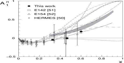
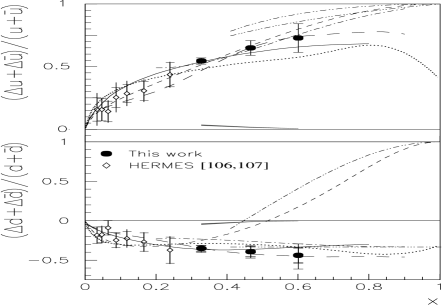
Figure 10: Left: Recent data on ${\cal A}_{1}^{n}$ from the E99-117 experiment Zheng et al. (2004a, b). Right: extracted polarization asymmetries for $u+\bar{u}$ and $d+\bar{d}$. For more details and references on the various model predictions, see Zheng et al. (2004a, b).

IX THE SPIN-FLAVOUR STRUCTURE OF THE PROTON

IX.1 The valence region and large $x$

The large $x$ region ($x$ close to one) is very interesting and particularly sensitive to the valence structure of the nucleon. Valence quarks dominate deep inelastic structure functions for large and intermediate $x$ (greater than about 0.2). Experiments at Jefferson Lab are making the first precision measurements of the proton’s spin structure at large $x$ – see Fig.10

QCD motivated predictions for the large $x$ region exist based on perturbative QCD counting rules and quarks models of the proton’s structure based on SU(6) [flavour SU(3) $\otimes$ spin SU(2)] and scalar diquark dominance. We give a brief explanation of these approaches.

1. Perturbative QCD counting rules predict that the parton distributions should behave as a power series expansion in $(1-x)$ when $x\rightarrow 1$ Brodsky et al. (1995); Farrar and Jackson (1975). The fundamental principle behind these counting rules results is that for the leading struck quark to carry helicity polarized in the same direction as the proton the spectator pair should carry spin zero, whence they are bound through longitudinal gluon exchange. For the struck quark to be polarized opposite to the direction of the proton the spectator pair should be in a spin one state, and in this case one has also to consider the effect of transverse gluon exchange. Calculation shows that this is supressed by a factor of $(1-x)^{2}$. We use $q^{\uparrow}(x)$ and $q^{\downarrow}(x)$ to denote the parton distributions polarized parallel and antiparallel to the polarized proton. One finds Brodsky et al. (1995)

   $$q^{\uparrow\downarrow}(x)\rightarrow(1-x)^{2n-1+2\Delta S_{z}},\ \ \ \ (x\rightarrow 1).$$ (140)

   Here $n$ is the number of spectators and $\Delta S_{z}$ is the difference between the polarization of the struck quark and the polarization of the target nucleon. When $x\rightarrow 1$ the QCD counting rules predict that the structure functions should be dominated by valence quarks polarized parallel to the spin of the nucleon. The ratio of polarized to unpolarized structure functions should go to one when $x\rightarrow 1$. For the helicity parallel valence quark distribution one predicts

   $$q^{\uparrow}(x)\sim(1-x)^{3},\ \ \ \ \ (x\rightarrow 1)$$ (141)

   whereas for the helicity anti-parallel distribution one obtains

   $$q^{\downarrow}(x)\sim(1-x)^{5},\ \ \ \ \ (x\rightarrow 1).$$ (142)

   Sea distributions are suppressed and the leading term starts as $(1-x)^{5}$.

2. Scalar diquark dominance is based on the observation that, within the context of the SU(6) wavefunction of the proton in Eq. (9), one gluon exchange tends to make the mass of the scalar diquark pair lighter than the vector spin-one diquark combination. One-gluon exchange offers an explanation of the nucleon-$\Delta$ mass splitting and has the practical consequence that in model calculations of deep inelastic structure functions the scalar diquark term ${1\over\sqrt{2}}|u\uparrow(ud)_{S=0}\rangle$ in Eq.(9) dominates the physics at large Bjorken $x$ Close and Thomas (1988).

In the large $x$ region ($x$ close to one) where sea quarks and gluons can be neglected the neutron and proton spin asymmetries are given by

$${\cal A}_{1}^{n}={\Delta u+4\Delta d\over u+4d},\ \ \ \ \ \ \ \ \ \ {\cal A}_{1}^{p}={4\Delta u+\Delta d\over 4u+d}.$$ (143)

Rearranging these expressions one obtains formulae for the separate up and down quark distributions in the proton:

$${\Delta u\over u} = {4\over 15}{\cal A}_{1}^{p}(4+{d\over u})-{1\over 15}{\cal A}_{1}^{n}(1+4{d\over u})$$

$${\Delta d\over d} = {4\over 15}{\cal A}_{1}^{n}(4+{u\over d})-{1\over 15}{\cal A}_{1}^{p}(1+4{u\over d}).$$ (144)

The predictions of perturbative QCD counting rules and scalar diquark dominance models for the large $x$ limit of these asymmetries are given in Table 1. On the basis of both perturbative QCD and SU(6), one expects the ratio of polarized to unpolarized structure functions, ${\cal A}_{1n}$, should approach 1 as $x\rightarrow 1$ Melnitchouk and Thomas (1996); Isgur (1999). It is vital to test this prediction. If it fails we understand nothing about the valence spin structure of the nucleon.

Table 1: QCD motivated model predictions for the large $x$ limit of deep inelastic spin asymmetries and parton distributions.

Model	$\Delta u/u$	$\Delta d/d$	${\cal A}_{1}^{p}$	${\cal A}_{1}^{n}$	$d/u$
SU(6)	${2\over 3}$	-${1\over 3}$	${5\over 9}$	0	${1\over 2}$
Broken SU(6), scalar diquark	1	-${1\over 3}$	1	1	0
QCD Counting Rules	1	1	1	1	${1\over 5}$

Interesting new data from the Jefferson Laboratory Hall A Collaboration the neutron asymmetry ${\cal A}_{1}^{n}$ Zheng et al. (2004a) are shown in Fig. 10. This data shows a clear trend for ${\cal A}_{1}^{n}$ to become positive at large $x$. The crossover point where ${\cal A}_{1}^{n}$ changes sign is particularly interesting because the value of $x$ where this occurs in the neutron asymmetry is the result of a competition between the SU(6) valence structure Close and Thomas (1988) and chiral corrections Schreiber and Thomas (1988); Steffens (1995). Fig. 10 also shows the extracted valence polarization asymmetries. The data are consistent with constituent quark models with scalar diquark dominance which predict $\Delta d/d\to-1/3$ at large $x$, while perturbative QCD counting rules predictions (which neglect quark orbital angular momentum) give $\Delta d/d\to 1$ and tend to deviate from the data, unless the convergence to 1 sets in very late.

A precision measurement of ${\cal A}_{1n}$ up to $x\sim 0.8$ will be possible following the 12 GeV upgrade of Jefferson Laboratory Meziani (2002).

IX.2 The isovector part of $g_{1}$

Constituent quark model predictions for $g_{1}$ are observed to work very well in the isovector channel. First, as highlighted in Section III.B above, the Bjorken sum rule which relates the first moment of the isovector part of $g_{1}$, $(g_{1}^{p}-g_{1}^{n})$, to the isovector axial charge $g_{A}^{(3)}$ has been confirmed in polarized deep inelastic scattering experiments at the level of 10% Windmolders (1999). Second, looking beyond the first moment, one finds the following intriguing observation about the shape of $(g_{1}^{p}-g_{1}^{n})$. Figure 11 shows $2x(g_{1}^{p}-g_{1}^{n})$ (SLAC data) together with the isovector structure function $(F_{2}^{p}-F_{2}^{n})$ (NMC data). The ratio $R_{(3)}=2x(g_{1}^{p}-g_{1}^{n})/(F_{2}^{p}-F_{2}^{n})$ is plotted in Fig. 12. It measures the ratio of polarized to unpolarized isovector quark distributions. In the QCD parton model

$$2x(g_{1}^{p}-g_{1}^{n})={1\over 3}x\Biggl{[}(u+{\overline{u}})^{\uparrow}-(u+{\overline{u}})^{\downarrow}-(d+{\overline{d}})^{\uparrow}+(d+{\overline{d}})^{\downarrow}\Biggr{]}$$ (145)

and

$$(F_{2}^{p}-F_{2}^{n})={1\over 3}x\Biggl{[}(u+{\overline{u}})^{\uparrow}+(u+{\overline{u}})^{\downarrow}-(d+{\overline{d}})^{\uparrow}-(d+{\overline{d}})^{\downarrow}\Biggr{]}.$$ (146)

The data reveal a large isovector contribution in $g_{1}$ and the ratio $R_{(3)}$ is observed to be approximately constant (at the value $\sim 5/3$ predicted by SU(6) constituent quark models) for $x$ between 0.03 and 0.2, and goes towards one when $x\rightarrow 1$ (consistent with the prediction of both QCD counting rules and scalar diquark dominance models). The small $x$ part of this data is very interesting. The area under $(F_{2}^{p}-F_{2}^{n})/2x$ is determined by the Gottfried integral Gottfried (1967); Arneodo et al. (1994) and is about 25% suppressed relative to the simple SU(6) prediction (by the pion cloud, Pauli blocking, … ). The area under $(g_{1}^{p}-g_{1}^{n})$ is fixed by the Bjorken sum rule (and is also about 25% suppressed relative to the SU(6) prediction – the suppression here being driven by relativistic effects in the nucleon and by perturbative QCD corrections to the Bjorken sum-rule). Given that perturbative QCD counting rules or scalar diquark models work and assuming that the ratio $R_{(3)}$ takes the constituent quark prediction at the canonical value of $x\sim{1\over 3}$, one finds Bass (1999) that the observed shape of $g_{1}^{p}-g_{1}^{n}$ is almost required to reproduce the area under the Bjorken sum rule (which is determined by the physical value of $g_{A}^{(3)}$ — a non-perturbative constraint)! The constant ratio in the low to medium $x$ range contrasts with the naive Regge prediction using $a_{1}$ exchange (and no hard-pomeron $a_{1}$ cut) that the ratio $R_{(3)}$ should fall and be roughly proportional to $x$ as $x\rightarrow 0$. It would be very interesting to have precision measurements of $g_{1}$ at high energy and low $Q^{2}$ from a future polarized $ep$ collider to test the various scenarios how small $x$ dynamics might evolve through the transition region and the application of spin dependent Regge theory.

Figure 11: The isovector structure functions $2xg_{1}^{(p-n)}$ (SLAC data) and $F_{2}^{(p-n)}$ (NMC) from Bass (1999).

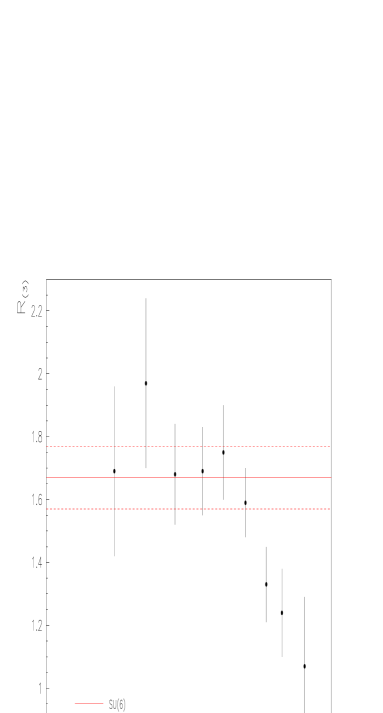
Figure 12: The ratio $R_{(3)}=2xg_{1}^{(p-n)}/F_{2}^{(p-n)}$ from Bass (1999).

IX.3 QCD fits to $g_{1}$ data

In deep inelastic scattering experiments the different $x$ data points on $g_{1}$ are each measured at different values of $Q^{2}$, viz. $x_{\rm expt.}(Q^{2})$. One has to evolve these experimental data points to the same value of $Q^{2}$ in order to test the Bjorken Bjorken (1966, 1970) and Ellis-Jaffe Ellis and Jaffe (1974) sum-rules. DGLAP evolution is frequently used in analyses of polarized deep inelastic data to achieve this.

The $\lambda^{2}$ dependence of the parton distributions is given by the DGLAP equations Altarelli and Parisi (1977)

$${d\over dt}\Delta\Sigma(x,t) = {\alpha_{s}(t)\over 2\pi}\biggl{[}\int_{x}^{1}{dy\over y}\Delta P_{qq}({x\over y})\Delta\Sigma(y,t)$$

$$\ \ \ \ \ \ \ \ \ \ +\ 2f\int_{x}^{1}{dy\over y}\Delta P_{qg}({x\over y})\Delta g(y,t)\biggr{]}$$

$${d\over dt}\Delta g(x,t) = {\alpha_{s}(t)\over 2\pi}\biggl{[}\int_{x}^{1}{dy\over y}\Delta P_{gq}({x\over y})\Delta\Sigma(y,t)$$

$$\ \ \ \ \ \ \ \ \ \ \ \ \ +\int_{x}^{1}{dy\over y}\Delta P_{gg}({x\over y})\Delta g(y,t)\ \biggr{]}$$

where $\Sigma(x,t)=\sum_{q}\Delta q(x,t)$ and $t=\ln\lambda^{2}$. The splitting functions $P_{ij}$ in Eq.(63) have been calculated at leading-order by Altarelli and Parisi Altarelli and Parisi (1977) and at next-to-leading order by Mertig, Zijlstra and van Neerven Mertig (1996); Zijlstra and van Neerven (1994) and Vogelsang Vogelsang (1996).

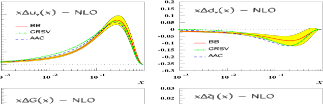
Figure 13: Polarized parton distribution functions from NLO pQCD (${\overline{\tt MS}}$) fits at $Q^{2}=4$GeV² using SU(3) flavour assumptions Stoesslein (2002).

Similar to the analysis that is carried out on unpolarized data, global NLO perturbative QCD analyses have been performed on the polarized structure function data sets. The aim is to extract the polarized quark and gluon parton distributions. These QCD fits are performed within a given factorization scheme, e.g. the “AB”, chiral invariant (CI) or JET and $\overline{\rm MS}$ schemes.

Let us briefly review these different factorization schemes.

Different factorization schemes correspond to different procedures for separating the phase space for photon-gluon fusion into “hard” and “soft” contributions in the convolution formula Eq. (LABEL:eqd80). In the QCD parton model analysis of photon gluon fusion that we discussed in Section XI.D using the cut-off on the transverse momentum squared, the polarized gluon contribution to the first moment of $g_{1}$ is associated with two-quark jet events carrying $k_{t}^{2}\sim Q^{2}$. The gluon coefficient function is given by $C^{(g)}_{{\rm PM}}=g_{1}^{(\gamma^{*}g)}|_{\rm hard}$ where $g_{1}^{(\gamma^{*}g)}|_{\rm hard}$ is taken from Eq.(122) with $Q^{2}\geq\lambda^{2}$ and $\lambda^{2}\gg P^{2},m^{2}$. This transverse-momentum cut-off scheme is sometimes called the “chiral invariant” (CI) Cheng (1996) or JET Leader et al. (1998) scheme.

Different schemes can be defined relative to this $k_{t}$ cut-off scheme by the transformation

$$C^{(g)}\biggl{(}x,{Q^{2}\over\lambda^{2}},\alpha_{s}(\lambda^{2})\biggr{)}$$

$$\rightarrow\ C^{(g)}\biggl{(}x,{Q^{2}\over\lambda^{2}},\alpha_{s}(\lambda^{2})\biggr{)}-{\tilde{C}}^{(g)}_{\rm scheme}\biggl{(}x,\alpha_{s}(\lambda^{2})\biggr{)}.$$

Here ${\tilde{C}}^{(g)}_{\rm scheme}$ shall be ${\alpha_{s}\over\pi}$ times a polynomial in $x$. The parton distributions transform as

$$\Delta\Sigma(x,\lambda^{2})_{\rm scheme}=\Delta\Sigma(x,\lambda^{2})_{\rm PM}$$

$$\ \ \ \ \ \ \ \ \ \ +f\int_{x}^{1}{dz\over z}\Delta g({x\over z},\lambda^{2})_{\rm PM}{\tilde{C}}^{(g)}_{\rm scheme}(z,\alpha_{s}(\lambda^{2}))$$

$$\Delta g(x,\lambda^{2})_{\rm scheme}=\Delta g(x,\lambda^{2})_{\rm PM}$$ (149)

so that the physical structure function $g_{1}$ is left invariant under the change of scheme. The virtuality and invariant-mass cut-off versions of the parton model that we discussed in Section XI.D correspond to different choices of scheme.

The ${\overline{\rm MS}}$ and AB schemes are defined as follows. In the ${\overline{\rm MS}}$ scheme the gluonic hard scattering coefficient is calculated using the operator product expansion with ${\overline{\rm MS}}$ renormalisation ’t Hooft and Veltman (1972). One finds Cheng (1996); Bass (1992a):

$$C^{(g)}_{{\overline{\rm MS}}}=C^{(g)}_{\rm PM}\ +\ {\alpha_{s}\over\pi}(1-x).$$ (150)

In this scheme $\int_{0}^{1}dx\ C^{(g)}_{\overline{\rm MS}}=0$ so that $\int_{0}^{1}dx\ \Delta g(x,\lambda^{2})$ decouples from $\int_{0}^{1}dxg_{1}$. This result corresponds to the fact that there is no gauge-invariant twist-two, spin-one, gluonic operator with $J^{P}=1^{+}$ to appear in the operator product expansion for the first moment of $g_{1}$. In the ${\overline{\rm MS}}$ scheme the contribution of $\int_{0}^{1}dx\ \Delta g$ to the first moment of $g_{1}$ is included into $\int_{0}^{1}dx\ \Sigma_{{\overline{\rm MS}}}(x,\lambda^{2})$. The AB scheme Ball et al. (1996) is defined by the formal operation of adding the $x$-independent term $-{\alpha_{s}\over 2\pi}$ to the ${\overline{\rm MS}}$ gluonic coefficient, viz.

$$C^{(g)}_{\rm AB}(x)=C^{(g)}_{{\overline{\rm MS}}}\ -\ {\alpha_{s}\over 2\pi}.$$ (151)

In the $\overline{\rm MS}$ scheme the polarized gluon distribution does not contribute explictly to the first moment of $g_{1}$. In the AB and JET schemes on the other hand the polarized gluon (axial anomaly contribution) $\alpha_{s}\Delta g$ does contribute explicitly to the first moment since $\int_{0}^{1}dx\ C^{(g)}=-{\alpha_{s}\over 2\pi}$.

For the SMC data one finds for the $\overline{\rm MS}$ (AB) scheme at a $Q^{2}$ of 1 GeV² Adeva et al. (1998b): $\Delta\Sigma=0.19\pm 0.05(0.38\pm 0.03)$ and $\Delta g=0.25^{+0.29}_{-0.22}(1.0^{+1.2}_{-0.3})$ where $\Delta\Sigma=(\Delta u+\Delta d+\Delta s)$. The main source of error in the QCD fits comes from lack of knowledge about $g_{1}$ in the small $x$ region and (theoretical) the functional form chosen for the quark and gluon distributions in the fits. Note that these QCD fits in both the AB and ${\overline{\rm MS}}$ schemes give values of $\Delta\Sigma$ which are smaller than the Ellis-Jaffe value 0.6.

New fits are now being produced taking into account all the available data including new data from polarized semi-inclusive deep inelastic scattering. Typical polarized distributions extracted from the fits are shown in Fig. 13. Given the uncertainties in the fits, values of $\Delta g$ are extracted ranging between about zero and +2. In these pQCD analyses one ends up with a consistent picture of the proton spin: the low value of $\Delta\Sigma$ may be compensated by a large polarized gluon. The precision on $\Delta g$ is however still rather modest. Moreover, it is vital to validate this model with direct measurements of $\Delta g$, as we discuss in Section IX.E below. Also, the first moments depend on integrations from $x=0$ to 1. Perhaps there is an additional component at very small $x$?

IX.4 Polarized quark distributions and semi-inclusive polarized deep inelastic scattering

As noted above, there are several possible mechanisms for producing sea quarks in the nucleon: photon-gluon fusion, the meson cloud of the nucleon, instantons, … In general the different dynamics will produce polarized sea with different $x$ and transverse momentum dependence.

Semi-inclusive measurements of fast pions and kaons in the current fragmentation region with final state particle identification can be used to reconstruct the individual up, down and strange quark contributions to the proton’s spin Close (1978); Close and Milner (1991); Frankfurt et al. (1989). In contrast to inclusive polarized deep inelastic scattering where the $g_{1}$ structure function is deduced by detecting only the scattered lepton, the detected particles in the semi-inclusive experiments are high-energy (greater than 20% of the energy of the incident photon) charged pions and kaons in coincidence with the scattered lepton. For large energy fraction $z=E_{h}/E_{\gamma}\rightarrow 1$ the most probable occurence is that the detected $\pi^{\pm}$ and $K^{\pm}$ contain the struck quark or antiquark in their valence Fock state. They therefore act as a tag of the flavour of the struck quark Close (1978).

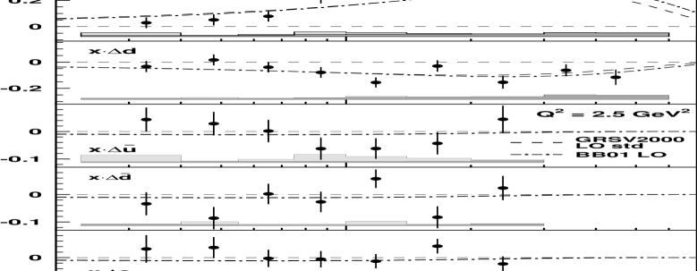
Figure 14: Recent Hermes results Airapetian et al. (2004) for the quark and antiquark polarizations extracted from semi-inclusive DIS.

In leading order (LO) QCD the double-spin asymmetry for the production of hadrons $h$ in semi-inclusive polarized $\gamma^{*}$ polarized proton collisons is:

$$A_{1p}^{h}(x,Q^{2})\simeq{\sum_{q,h}e_{q}^{2}\Delta q(x,Q^{2})\int_{z_{\rm min}}^{1}D_{q}^{h}(z,Q^{2})\over\sum_{q,h}e_{q}^{2}q(x,Q^{2})\int_{z_{\rm min}}^{1}D_{q}^{h}(z,Q^{2})}$$ (152)

where $z_{\rm min}\sim 0.2$. Here

$$D_{q}^{h}(z,Q^{2})=\int dk_{t}^{2}D_{q}^{h}(z,k_{t}^{2},Q^{2})$$ (153)

is the fragmentation function for the struck quark or antiquark to produce a hadron $h$ ($=\pi^{\pm},K^{\pm}$) carrying energy fraction $z=E_{h}/E_{\gamma}$ in the target rest frame; $\Delta q(x,Q^{2})$ is the quark (or antiquark) polarized parton distribution and $e_{q}$ is the quark charge. Note the integration over the transverse momentum $k_{t}$ of the final-state hadrons Close and Milner (1991). (In practice this integration over $k_{t}$ is determined by the acceptance of the experiment.) Since pions and kaons have spin zero, the fragmentation functions are the same for both polarized and unpolarized leptoproduction. NLO corrections to Eq. (152) are discussed in de Florian et al. (1998); de Florian and Sassot (2000).

This programme for polarized deep inelastic scattering was pioneered by the SMC Adeva et al. (1998c) and HERMES Ackerstaff et al. (1999) Collaborations with new recent measurements from HERMES reported in Airapetian et al. (2004, 2005a). Fig. 14 shows the latest results on the flavor separation from HERMES Airapetian et al. (2004), which were obtained using a leading-order (naive parton model) Monte-Carlo code based “purity” analysis. The polarization of the up and down quarks are positive and negative respectively, while the sea polarization data are consistent with zero and not inconsistent with the negative sea polarization suggested by inclusive deep inelastic data within the measured $x$ range Glück et al. (2001); Blümlein and Böttcher (2002). However, there is also no evidence from this semi-inclusive analysis for a large negative strange quark polarization. For the region $0.023<x<0.3$ the extracted $\Delta s$ integrates to the value $+0.03\pm 0.03\pm 0.01$ which contrasts with the negative value for the polarized strangeness (6) extracted from inclusive measurements of $g_{1}$. It will be interesting to see whether this effect persists in forthcoming semi-inclusive data from COMPASS. The HERMES data also favour an isospin symmetric sea $\Delta{\bar{u}}-\Delta{\bar{d}}$, but with large uncertainties.

An important issue for semi-inclusive measurements is the angular coverage of the detector Bass (2003a). The non-valence spin-flavour structure of the proton extracted from semi-inclusive measurements of polarized deep inelastic scattering may depend strongly on the transverse momentum (and angular) acceptance of the detected final-state hadrons which are used to determine the individual polarized sea distributions. The present semi-inclusive experiments detect final-state hadrons produced only at small angles from the incident lepton beam (about 150 mrad angular coverage) The perturbative QCD “polarized gluon interpretation” Efremov and Teryaev (1988); Altarelli and Ross (1988) of the inclusive measurement (6) involves physics at the maximum transverse momentum Carlitz et al. (1988); Bass (2003a) and large angles – see Fig.9. Observe the small value for the light-quark sea polarization at low transverse momentum and the positive value for the integrated strange sea polarization at low $k_{t}^{2}$: $k_{t}<1.5$GeV at the HERMES $Q^{2}=2.5$GeV². When we relax the transverse momentum cut-off, increasing the acceptance of the experiment, the measured strange sea polarization changes sign and becomes negative (the result implied by fully inclusive deep inelastic measurements). For HERMES the average transverse momentum of the detected final-state fast hadrons is less than about 0.5 GeV whereas for SMC the $k_{t}$ of the detected fast pions was less than about 1 GeV. Hence, there is a question whether the leading-order sea quark polarizations extracted from semi-inclusive experiments with limited angular resolution fully include the effect of the axial anomaly or not.

Recent theoretical studies motivated by this data include also possible effects associated spin dependent fragmentation functions Kretzer et al. (2001), possible higher twist effects in semi-inclusive deep inelastic scattering, and possible improvements in the Monte Carlo Kotzinian (2003).

The dependence on the details of the fragmentation process limits the accuracy of the method above. At RHIC Bunce et al. (2000) the polarization of the $u,\overline{u},d$ and $\overline{d}$ quarks in the proton will be measured directly and precisely using $W$ boson production in $u\overline{d}\rightarrow W^{+}$ and $d\overline{u}\rightarrow W^{-}$. The charged weak boson is produced through a pure V-A coupling and the chirality of the quark and anti-quark in the reaction is fixed. A parity violating asymmetry for $W^{+}$ production in $pp$ collisions can be expressed as

$$A(W^{+})=\frac{\Delta u(x_{1})\overline{d}(x_{2})-\Delta\overline{d}(x_{1})u(x_{2})}{u(x_{1})\overline{d}(x_{2})+\overline{d}(x_{1})u(x_{2})}.$$ (154)

For $W^{-}$ production $u$ and $d$ quarks should be exchanged. The expression converges to $\Delta u(x)/u(x)$ and $-\Delta\overline{d}(x)/\overline{d}(x)$ in the limits $x_{1}\gg x_{2}$ and $x_{2}\gg x_{1}$ respectively. The momentum fractions are calculated as $x_{1}=\frac{M_{W}}{\sqrt{s}}e^{y_{W}}$ and $x_{2}=\frac{M_{W}}{\sqrt{s}}e^{-y_{W}}$, with $y_{W}$ the rapidity of the $W$. The experimental difficulty is that the $W$ is observed through its leptonic decay $W\rightarrow l\nu$ and only the charged lepton is observed. With the assumed integrated luminosity of 800 pb^-1 at $\sqrt{s}=500$ GeV, one can expect about 5000 events each for $W^{+}$ and $W^{-}$. The resulting measurement precision is shown in Fig. 15.

It has also been pointed out that neutrino factories would be an ideal tool for polarized quark flavour decomposition studies. These would allow one to collect large data samples of charged current events, in the kinematic region $(x,Q^{2})$ of present fixed target data Forte et al. (2001). A complete separation of all four flavours and anti-flavours would become possible, including $\Delta s(x,Q^{2})$.

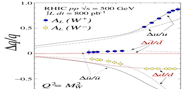
Figure 15: Expected sensitivity Bunce et al. (2000) for the flavor decomposition of quark and anti-quark polarizations at RHIC. Reprinted, with permission, from the Annual Reviews of Nuclear and Particle Science, Volume 50 (c)2000 by Annual Reviews www.annualreviews.org.

IX.5 The polarized gluon distribution $\Delta g(x,Q^{2})$

Motivated by the discovery of Altarelli and Ross (1988) and Efremov and Teryaev (1988) that polarized glue makes a scaling contribution to the first moment of $g_{1}$, $\alpha_{s}\Delta g\sim{\tt constant}$, there has been a vigorous and ambitious programme to measure $\Delta g$. The NLO QCD motivated fits to the inclusive $g_{1}$ data are suggestive that, perhaps, the net polarized glue might be positive but more direct measurements involving glue sensitive observables are needed to really extract the magnitude of $\Delta g$ and the shape of $\Delta g(x,Q^{2})$ including any possible nodes in the distribution function. Possible channels include gluon mediated processes in semi-inclusive polarized deep inelastic scattering and hard QCD processes in high energy polarized proton-proton collisions at RHIC.

COMPASS has been conceived to measure $\Delta g$ via the study of the photon-gluon fusion process, as shown in Fig. 16. The cross section of this process is directly related to the gluon density at the Born level. The experimental technique consists of the reconstruction of charmed mesons in the final state. COMPASS will also use the same process with high $p_{t}$ particles instead of charm to access $\Delta g$. This may lead to samples with larger statistics, but these have larger background contributions, namely from QCD Compton processes and fragmentation. The expected sensitivity on the measurement of $\Delta g/g$ from these experiments is estimated to be about $\delta(\Delta g/g)=0.1$ at $x_{g}\sim 0.1$.

Figure 16: c $\overline{\rm c}$ production in Photon Gluon Fusion

HERMES was the first to attempt to measure $\Delta g$ using high $p_{t}$ charged particles, as proposed for COMPASS above, and nearly real photons $\langle Q^{2}\rangle=0.06$GeV². The measurement is at the limit of where a perturbative treatment of the data can be expected to be valid, but the result is interesting: $\Delta g/g=0.41\pm 0.18\pm 0.03$ at an average $<x_{g}>=0.17$ Airapetian et al. (2000). The SMC Collaboration have performed a similar analysis for their own data keeping $Q^{2}>1$GeV². An average gluon polarization was extracted $\Delta g/g=-0.20\pm 0.28\pm 0.10$ at an average gluon momentum $x_{g}=0.07$ Adeva et al. (2004).

The hunt for $\Delta g$ is also one of the main physics drives for polarized RHIC. The key processes used here are high-$p_{t}$ prompt photon production $pp\rightarrow\gamma X$, jet production $pp\rightarrow$ jets $+X$, and heavy flavour production $pp\rightarrow c\overline{c}X,b\overline{b}X,J/\psi X$. Due to the first stage detector capabilities most emphasis has so far been put on the prompt photon channel. Measurements of $\Delta g/g$ are expected in the gluon $x$ range $0.03<x_{g}<0.3$.

These anticipated RHIC measurements of $\Delta g$ have inspired new theoretical developments aimed at implementing higher-order calculations of partonic cross-sections into global analyses of polarized parton distribution functions, which will benefit the analyses of future polarized $pp$ data to measure $\Delta g$. Hard polarized reactions at RHIC and the polarized parton distributions that they probe are summarized in Table II.

Table 2: Polarized partons from RHIC

reaction	LO subprocesses	partons probed	$x$ range
$pp\rightarrow{\rm jets}X$	$q{\overline{q}},qq,qg,gg\rightarrow{\rm jet}X$	$\Delta q,\Delta g$	$x>0.03$
$pp\rightarrow\pi X$	$q{\overline{q}},qq,gg\rightarrow\pi X$	$\Delta q,\Delta g$	$x>0.03$
$pp\rightarrow\gamma X$	$qg\rightarrow q\gamma$, $q{\overline{q}}\rightarrow g\gamma$	$\Delta g$	$x>0.03$
$pp\rightarrow Q{\overline{Q}}X$	$gg\rightarrow Q{\overline{Q}}$, $q{\overline{q}}\rightarrow Q{\overline{Q}}$	$\Delta g$	$x>0.01$
$pp\rightarrow W^{\pm}X$	$q{\overline{q}^{\prime}}\rightarrow W^{\pm}$	$\Delta u,\Delta{\overline{u}},\Delta d,\Delta{\overline{d}}$	$x>0.06$

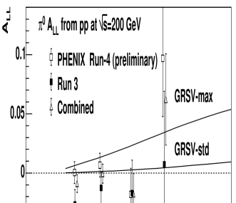
Figure 17: The PHENIX (preliminary Run-4) data Fukao (2005) for the spin asymmetry ${\cal A}_{LL}^{\pi}$ along with NLO perturbative QCD predictions for various $\Delta g$ Jäger et al. (2004)

In the first runs at RHIC the longitudinal double spin asymmetry for production of a leading pion $\pi^{0}$ with large transverse momentum has been used as a surrogate jet to investigate possible gluon polarization in the proton. NLO perturbative QCD corrections to this process have been calculated in de Florian (2003) and Jäger et al. (2003). The data from PHENIX Adler et al. (2004); Fukao (2005) are shown in Fig. 17 and are consistent with a significant (up to a few percent) negative asymmetry ${\cal A}^{\pi}_{LL}$ for pion transverse momentum $1<p_{t}<4$GeV in contrast with the predictions of leading twist perturbative QCD calculations which do provide a good description of the unpolarized cross-section in the same kinematics. It will be interesting to see whether this effect survives more precise data. The NLO perturbative QCD analysis of Jäger et al. (2004) suggests that the leading power in $p_{t}$ contribution to ${\cal A}^{\pi}_{LL}$ cannot be large and negative in the measured range of $p_{t}$ within the framework of perturbative QCD independent of the sign of $\Delta g$. One would need to invoke power suppressed contributions (though the leading power term seems to describe the corresponding unpolarized data) and/or non-perturbative effects. Increase in precision and data at higher pion $p_{t}$ (up to about 12 GeV) are expected from future runs.

Future polarized $ep$ colliders could add information in two ways: by extending the kinematic range for measurements of $g_{1}$ or by direct measurements of $\Delta g$. A precise measurement of $\Delta g$ is crucial for a full understanding of the proton spin problem. HERA has shown that large centre of mass energy allows several processes to be used to extract the unpolarized gluon distribution. These include jet and high $p_{t}$ hadron production, charm production both in DIS and photoproduction, and correlations between multiplicities of the current and target hemisphere of the events in the Breit frame. The most promising process for a direct extraction of $\Delta g$ is di-jet production  De Roeck et al. (1999); Rädel and De Roeck (2002). The underlying idea is to isolate boson-gluon fusion events where the gluon distribution enters at the Born level.

X TRANSVERSITY

There are three species of twist-two quark distributions in QCD. These are the spin independent distributions $q(x)$ measured in the unpolarized structure functions $F_{1}$ and $F_{2}$, the spin dependent distributions $\Delta q(x)$ measured in $g_{1}$ and the transversity distributions $\delta q(x)$.

The transversity distributions describe the density of transversely polarized quarks inside a transversely polarized proton Barone et al. (2002). Measuring transversity is an important experimental challenge in QCD spin physics. We briefly describe the physics of transversity and the programme to measure it.

The twist-two transversity distributions Ralston and Soper (1979); Artru and Mekhfi (1990); Jaffe and Ji (1992) can be interpreted in parton language as follows. Consider a nucleon moving with (infinite) momentum in the $\hat{e}_{3}$-direction, but polarized along one of the directions transverse to $\hat{e}_{3}$. Then $\delta q(x,Q^{2})$ counts the quarks with flavour $q$, momentum fraction $x$ and their spin parallel to the spin of a nucleon minus the number antiparallel. That is, in analogy with Eq. (LABEL:eqb28), $\delta q(x)$ measures the distribution of partons with transverse polarization in a transversely polarized nucleon, viz.

$$\delta q(x,Q^{2})=q^{\uparrow}(x)-q^{\downarrow}(x).$$ (155)

In a helicity basis, transversity corresponds to the helicity-flip structure shown in Fig. 18 making transversity a probe of chiral symmetry breaking Collins (1993b).

Figure 18: Transversity in helicity basis.

The first moment of the transversity distribution is proportional to the nucleon’s C-odd tensor charge, viz. $\delta q=\int_{0}^{1}dx\delta q(x)$ with

$$\langle p,s|\ {\bar{q}}i\sigma_{\mu\nu}\gamma_{5}q\ |p,s\rangle=(1/M)(s_{\mu}p_{\nu}-s_{\nu}p_{\mu})\delta q.$$ (156)

Transversity is C-odd and chiral-odd.

If quarks moved non-relativistically in the nucleon $\delta q$ and $\Delta q$ would be identical since rotations and Euclidean boosts commute and a series of boosts and rotations can convert a longitudinally polarized nucleon into a transversely polarized nucleon at infinite momentum. The difference between the transversity and helicity distributions reflects the relativistic character of quark motion in the nucleon. In the MIT Bag Model this effect is manifest as follows. The lower component of the Dirac spinor enters the relativistic spin depolarization factor with the opposite sign to $\Delta q$ because of the extra factor of $\gamma_{\mu}$ in the tensor charge Jaffe and Ji (1992). That is, the relativistic depolarization factor $N^{2}\int_{0}^{R}drr^{2}(f^{2}-{1\over 3}g^{2})$ for $\Delta q$ mentioned in Section I.A is replaced by $N^{2}\int_{0}^{R}drr^{2}(f^{2}+{1\over 3}g^{2})$ for $\delta q$ where $\psi={N\over\sqrt{4\pi}}\biggl{(}{f\atop i\sigma.{\hat{r}}g}\biggr{)}$ is the Dirac spinor.

Little is presently known about the shape of the transversity distributions. However some general properties can be deduced from QCD arguments. The spin distributions $\Delta q(x)$ and $\delta q(x)$ have opposite charge conjugation properties: $\Delta q(x)$ is C-even whereas $\delta q(x)$ is C-odd. The spin dependent quark and gluon helicity distributions ($\Delta q$ and $\Delta g$) mix under $Q^{2}$-evolution. In contrast, there is no analog of gluon transversity in the nucleon so $\delta q$ evolves without mixing, like a non-singlet parton distribution function. Not coupling to glue or perturbative $\bar{q}q$ pairs, $\delta q(x)$ and the tensor charge promise to be more quark-model–like than the singlet axial-charge (though they are both scale dependent) and should be an interesting contrast Jaffe (2001). Under QCD evolution the moments $\int_{0}^{1}dxx^{n}\delta q(x,Q^{2})$ decrease with increasing $Q^{2}$. In leading order QCD the transversity distributions are bounded above by Soffer’s inequality Soffer (1995)

$$|\delta q(x,Q^{2})|\leq{1\over 2}\biggl{[}q(x,Q^{2})+\Delta q(x,Q^{2})\biggr{]}.$$ (157)

Experimental study of transversity distributions at leading-twist requires observables which are the product of two objects with odd chirality – the transversity distribution and either a second transversity distribution or a chiral odd fragmentation function. In proton-proton collisions the transverse double spin asymmetry, ${\cal A}_{TT}$, is proportional to $\delta q\delta\bar{q}$ with even chirality. However the asymmetry is small requiring very large luminosity samples because of the large background from gluon induced processes in unpolarized scattering. The most promising process to measure this double spin asymmetry is perhaps Drell-Yan production.

Transverse single spin asymmetries ${\cal A}_{N}$ are also being studied with a view to extracting information about transversity distributions. Here the focus is on single hadron production with a transversely polarized proton beam or target in $pp$ and $ep$ collisions. The key process is

$$A(p,{\vec{s}}_{t})+B(p^{\prime})\rightarrow C(l)+X$$ (158)

where $C$ is typically a pion produced at large transverse momentum $l_{t}$.

Several mechanisms for producing these transverse single spin asymmetries have been discussed in the literature. The asymmetries ${\cal A}_{N}$ are powered suppressed in QCD. Leading $l_{t}$ behaviour of the produced pion can occur from the Collins Collins (1993b) and Sivers Sivers (1991) effects plus twist-3 mechanisms Qiu and Sterman (1999). The Collins effect involves the chiral-odd twist-2 transversity distribution in combination with a chiral-odd fragmentation function for the high $l_{t}$ pion in the final state. It gives a possible route to measuring transversity. The Sivers effect is associated with intrinsic quark transverse momentum in the initial state. The challenge is to disentangle these effects from experimental data.

Factorization for transverse single spin processes in proton-proton collisions has been derived by Qiu and Sterman (1999) in terms of the convolution of a twist-two parton distribution from the unpolarized hadron, a twist-three quark-gluon correlation function from the polarized hadron, and a short distance partonic hard part calculable in perturbative QCD. We refer to Anselmino et al. (2005) for a discussion of factorization for processes such as the Collins and Sivers effects involving unintegrated transverse momentum dependent parton and fragmentation functions.

We next outline the Collins and Sivers effects.

The Collins effect Collins (1993b) uses properties of fragmentation to probe transversity. The idea is that a pion produced in fragmentation will have some transverse momentum with respect to the momentum $k$ of the transversely polarized fragmenting parent quark. One finds a correlation of the form $\;i\vec{s}_{t}\cdot(\vec{l}^{(\pi)}\times\vec{k}_{t})$. The Collins fragmentation function associated with this correlation is chiral-odd and T-even. It combines with the chiral-odd transversity distribution to contribute to the transverse single spin asymmetry.

For the Sivers effect Sivers (1991) the $k_{t}$ distribution of a quark in a transversely polarized hadron can generate an azimuthal asymmetry through the correlation $\,\vec{s}_{t}\cdot(\vec{p}\times\vec{k}_{t})$. In this process final state interaction (FSI) of the active quark produces the asymmetry before it fragments into hadrons Brodsky et al. (2002); Burkardt and Hwang (2004); Yuan (2003); Bachetta et al. (2004). This process involves a $k_{t}$ unintegrated quark distribution function in the transversely polarized proton. The dependence on intrinsic quark transverse momentum means that this Sivers process is related to quark orbital angular momentum in the proton Burkardt (2002). The Sivers distribution function is chiral-even and T-odd. The possible role of quark orbital angular momentum in understanding transverse single-spin asymmetries is also discussed in Boros et al. (1993).

The Sivers process is associated with the gauge link in operator definitions of the parton distributions. The gauge link factor is trivial and equal to one for the usual $k_{t}$ integrated parton distributions measured in inclusive polarized deep inelastic scattering. However, for $k_{t}$ unintegrated distributions the gauge link survives in a transverse direction at light-cone component $\xi^{-}=\infty$. The gauge-link plays a vital role in the Sivers process Burkardt (2005). Without it (e.g. in the pre-QCD “naive” parton model) time reversal invariance implies vanishing Sivers effect Ji and Yuan (2002); Belitsky et al. (2003a). The Sivers distribution function has the interesting property that it has the opposite sign in deep inelastic scattering and Drell-Yan reactions Collins (2002). It thus violates the universality of parton distribution functions.

Figure 19: Recent Star results for the asymmetry $A_{\mathrm{N}}$ in $pp\to\pi^{0}X$ in the forward Feynman-$x_{F}$ region Adams et al. (2004).

The FermiLab experiment E704 found large transverse single-spin asymmetries ${\cal A}_{N}$ for $\pi$ and $\Lambda$ production in proton-antiproton collisions at centre of mass energy $\sqrt{s}=20$GeV Adams et al. (1991a, b); Bravar et al. (1996). Large transverse single-spin asymmetries have also been observed in recent data from the STAR collaboration at RHIC in proton-proton collisions at centre of mass energy $\sqrt{s}=200$GeV Adams et al. (2004) – see Figure 19 which also shows various theoretical predictions. In a recent paper Anselmino et al. (2005) take into account intrinsic parton motion in the distribution and fragmentation functions as well as in the elementary dynamics and argue that the Collins mechanism may be strongly suppressed at large Feynman $x_{F}$ in this process. The Sivers effect is not suppressed and remains a candidate to explain the data. Higher-twist contributions Qiu and Sterman (1999) from quark-gluon correlations may also be important.

The HERMES experiment has taken measurements of charged pion production in $ep$ scattering with transverse target polarization Airapetian et al. (2005b). This data has been analysed for possible contributions from the Collins and Sivers effects. The azimuthal distribution of the final state pions with respect to the virtual photon axis is expected to carry information about transversity through the Collins effect and about intrinsic transverse momentum in the proton through the Sivers effect. In this analsis one first writes the transverse single-spin asymmetry ${\cal A}_{N}$ as the sum

$${\cal A}_{N}(x,z)={\cal A}_{N}^{\rm Collins}+{\cal A}_{N}^{\rm Sivers}+...$$ (159)

where

$${\cal A}_{N}^{\rm Collins}\propto|{\vec{s}}_{t}|\sin(\phi+\phi_{S})\frac{\sum_{q}e_{q}^{2}\delta q(x)H_{1}^{\perp,q}(z)}{\sum_{q}e^{2}_{q}q(x)D_{q}^{\pi}(z)}$$ (160)

and

$${\cal A}_{N}^{\rm Sivers}\propto|{\vec{s}}_{t}|\sin(\phi-\phi_{S})\frac{\sum_{q}e_{q}^{2}f_{1T}^{\perp,q}D_{q}^{\pi}(z)}{\sum_{q}e^{2}_{q}q(x)D_{q}^{\pi}(z)}$$ (161)

denote the contributions from the Collins and Sivers effects. Here $\phi$ is the angle between the lepton direction and the $(\gamma^{*}\pi)$ plane and $\phi_{S}$ is the angle between the lepton direction and the transverse target spin; $H_{1}^{\perp q}$ is the Collins function for a quark of flavour $q$, $f_{1T}^{\perp,q}$ is the Sivers distribution function, and $D_{q}^{\pi}$ is the regular spin independent fragmentation function. When one projects out the two terms with different azimuthal angular dependence the HERMES analysis suggests that both the Collins and Sivers effects are present in the data. Futhermore, the analysis suggests the puzzling result that the “favoured” (for $u\rightarrow\pi^{+}$) and “unfavoured” (for $d\rightarrow\pi^{+}$) Collins fragmentation functions may contribute with equal weight (and opposite sign) Airapetian et al. (2005b).

Other processes and experiments will help to clarrify the importance of the Collins and Sivers processes. Additional studies of the Collins effect have been proposed in $e^{+}e^{-}$ collisions using the high statistics data samples of BABAR and BELLE. The aim is to measure two relevant fragmentation functions: the Collins function $H_{1}^{\perp}$ and the interference fragmentation functions $\delta\hat{q}^{h_{1},h_{2}}$. For the first, one measures the fragmentation of a transversely polarized quark into a charged pion and the azimuthal distribution of the final state pion with respect to the initial quark momentum (jet-axis). For the second, one measures the fragmentation of transversely polarized quarks into pairs of hadrons in a state which is the superposition of two different partial wave amplitudes; e.g. $\pi^{+},\pi^{-}$ pairs in the $\rho$ and $\sigma$ invariant mass region Collins et al. (1994); Jaffe et al. (1988). The high luminosity and particle identification capabilities of detectors at B-factories makes these measurements possible.

The Sivers distribution function might be measurable through the transverse single spin asymmetry ${\cal A}_{N}$ for D meson production generated in $p^{\uparrow}p$ scattering Anselmino et al. (2004). Here the underlying elementary processes guarantee the absence of any polarization in the final partonic state so that there is no contamination from Collins like terms. Large dominance of the process $gg\rightarrow c{\bar{c}}$ process at low and intermediate $x_{F}$ offers a unique opportunity to measure the gluonic Sivers distribution function. The gluonic Sivers function could also be extracted from back-to-back correlations in the azimuthal angle of jets in collisions of unpolarized and transversely polarized proton beams at RHIC Boer and Vogelsang (2004).

Measurements with transversely polarized targets have a bright future and are already yielding surprises. The results promise to be interesting and to teach us about transversity and about the role of quark transverse momentum in the structure of the proton and fragmentation processes.

XI DEEPLY VIRTUAL COMPTON SCATTERING AND EXCLUSIVE PROCESSES

XI.1 Orbital angular momentum

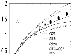
Figure 20: Jefferson Lab data on the the ratio of the proton’s Pauli to Dirac form-factors Gayou et al. (2002).

So far in this review we have concentrated on intrinsic spin in the proton. The orbital angular momentum structure of the proton is also of considerable interest and much effort has gone into devising ways to measure it. The strategy involves the use of hard exclusive reactions and the formalism of generalized parton distributions (GPDs) which describes deeply virtual Compton scattering (DVCS) and meson production (DVMP). Possible hints of quark orbital angular momentum are also suggested by recent form-factor measurements at Jefferson Laboratory Jones et al. (2000); Gayou et al. (2002) – see Fig.20. The ratio of the spin-flip Pauli form-factor to the Dirac form-factor is observed to have a $1/\sqrt{Q^{2}}$ behaviour in the measured region in contrast with the $1/Q^{2}$ behaviour predicted by QCD Counting Rules (helicity conservation neglecting angular momentum), viz. $F_{1}\sim 1/Q^{4}$ and $F_{2}\sim 1/Q^{6}$ Brodsky and Lepage (1980). However, this data can also be fit with the formula

$$\frac{F_{2}(Q^{2})}{F_{1}(Q^{2})}=\frac{\mu_{A}}{1+(Q^{2}/c)\ln^{b}(1+Q^{2}/a)}$$ (162)

(with $\mu_{A}=1.79$, $a=4m_{\pi}^{2}=0.073$ GeV², $b=-0.5922$, $c=0.9599$ GeV²) prompting the question at which $Q^{2}$ the Counting Rules prediction is supposed to work and at which $Q^{2}$ higher twist effects can be neglected Brodsky (2002a). At this point it is interesting to recall that the simple Counting Rules prediction fails to describe the large $x$ behaviour of $\Delta d/d$ in the presently measured JLab kinematics – Section IX.A.

A $1/Q$ behaviour for $\frac{F_{2}(Q^{2})}{F_{1}(Q^{2})}$ is found in a light-front Cloudy Bag calculation Miller and Frank (2002); Miller (2002) and in quark models with orbital angular momentum Ralston and Jain (2004); Ralston et al. (2002). A new perturbative QCD calculation which takes into account orbital angular momentum Belitsky et al. (2003b) gives $F_{2}/F_{1}\sim(\log^{2}Q^{2}/\Lambda^{2})/Q^{2}$ and also fits the Jefferson Lab data well. The planned 12 GeV upgrade at Jefferson Laboratory will enable us to measure these nucleon form-factors at higher $Q^{2}$ and the inclusive spin asymmetries at values of Bjorken $x$ closer to one, and thus probe deeper into the kinematic regions where QCD Counting Rules should apply. This data promises to be very interesting!

Deeply virtual Compton scattering (DVCS) provides a possible experimental tool to access the quark total angular momentum, $J_{q}$, in the proton through the physics of generalized parton distributions (GPDs)  Ji (1997a, b). The form-factors which appear in the forward limit $(t\rightarrow 0)$ of the second moment of the spin-independent generalized quark parton distribution in the (leading-twist) spin-independent part of the DVCS amplitude project out the quark total angular momentum defined through the proton matrix element of the QCD angular-momentum tensor. We explain this physics below.

DVCS studies have to be careful to chose the kinematics not to be saturated by a large Bethe-Heitler (BH) background where the emitted real photon is radiated from the electron rather than the proton. The HERMES and Jefferson Laboratory experiments measure in the kinematics where they expect to be dominated by the DVCS-BH interference term and observe the $\sin\phi$ azimuthal angle and helicity dependence expected for this contribution – see Fig.21. First measurements of the single spin asymmetry have been reported in  Airapetian et al. (2001); Stepanyan et al. (2001), which have the characteristics expected from the DVCS-BH interference.

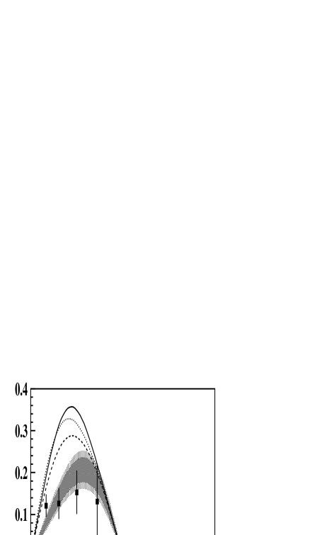
Figure 21: Recent data from HERMES (left) and the CLAS experiment at Jefferson Laboratory (right) in the realm of DVCS Bethe-Heitler interference. The $\sin\phi$ azimuthal dependence of the single spin asymmetry is clearly visible in the data Airapetian et al. (2001); Stepanyan et al. (2001).

XI.2 Generalized parton distributions

For exclusive processes such as DVCS or hard meson production the generalized parton distributions involve non-forward proton matrix elements Goeke et al. (2001); Ji (1998); Diehl (2003); Radyushkin (1997); Vanderhaeghen et al. (1998). The important kinematic variables are the virtuality of the hard photon $Q^{2}$, the momenta $p-\Delta/2$ of the incident proton and $p+\Delta/2$ of the outgoing proton, the invariant four-momentum transferred to the target $t=\Delta^{2}$, the average nucleon momentum $P$, the generalized Bjorken variable $k^{+}=xP^{+}$ and the light-cone momentum transferred to the target proton $\xi=-\Delta^{+}/2p^{+}$. The generalized parton distributions are defined as the light-cone Fourier transform of the point-split matrix element

$${P_{+}\over 2\pi}\int dy^{-}e^{-ixP^{+}y^{-}}\langle p^{\prime}|{\bar{\psi}}_{\alpha}(y)\psi_{\beta}(0)|p\rangle_{y^{+}=y_{\perp}=0}$$

$$={1\over 4}\gamma^{-}_{\alpha\beta}\biggl{[}H(x,\xi,\Delta^{2}){\bar{u}}(p^{\prime})\gamma^{+}u(p)$$

$$\ \ \ \ \ \ \ \ \ \ \ \ \ \ \ \ \ \ \ \ \ \ +E(x,\xi,\Delta^{2}){\bar{u}}(p^{\prime})\sigma^{+\mu}{\Delta_{\mu}\over 2M}u(p)\biggr{]}$$

$$\ \ \ +{1\over 4}(\gamma_{5}\gamma^{-})_{\alpha\beta}\biggl{[}{\tilde{H}}(x,\xi,\Delta^{2}){\bar{u}}(p^{\prime})\gamma^{+}\gamma_{5}u(p)$$

$$\ \ \ \ \ \ \ \ \ \ \ \ \ \ \ \ \ \ \ \ \ \ \ \ \ +{\tilde{E}}(x,\xi,\Delta^{2}){\bar{u}}(p^{\prime})\gamma_{5}{\Delta^{+}\over 2M}u(p)\biggr{]}.$$

(163)

(Here we work in the light-cone gauge $A_{+}=0$ so that the path-ordered gauge-link becomes trivial and equal to one to maintain gauge invariance through-out.)

The physical interpretation of the generalized parton distributions (before worrying about possible renormalization effects and higher order corrections) is the following. Expanding out the quark field operators in (163) in terms of light-cone quantized creation and annihilation operators one finds that for $x>\xi$ ($x<\xi$) the GPD is the amplitude to take a quark (anti-quark) of momentum $k-\Delta/2$ out of the proton and reinsert a quark (anti-quark) of momentum $k+\Delta/2$ into the proton some distance along the light-cone to reform the recoiling proton. In this region the GPD is a simple generalization of the usual parton distributions studied in inclusive and semi-inclusive scattering. In the remaining region $-\xi<x<\xi$ the GPD involves taking out (or inserting) a $q{\bar{q}}$ pair with momentum $k-\Delta/2$ and $-k-\Delta/2$ (or $k+\Delta/2$ and $-k+\Delta/2$) respectively. Note that the GPDs are interpreted as probability amplitudes rather than densities.

In the forward limit the GPDs $H$ and ${\tilde{H}}$ are related to the forward parton distributions studied in (polarized) deep inelastic scattering:

$$H(x,\xi,\Delta^{2})|_{\xi=\Delta^{2}=0} = q(x)$$

$${\tilde{H}}(x,\xi,\Delta^{2})|_{\xi=\Delta^{2}=0} = \Delta q(x)$$ (164)

whereas the GPDs $E$ and ${\tilde{E}}$ have no such analogue. In the fully renormalized theory the spin dependent distributions ${\tilde{H}}$ and ${\tilde{E}}$ will be sensitive to the physics of the axial anomaly and, in this case, it is not easy to separate off an “anomalous component” because the non-forward matrix elements of the gluonic Chern-Simons current are non-gauge-invariant even in the light-cone gauge $A_{+}=0$. Integrating over $x$ the first moments of the GPDs are related to the nucleon form-factors:

$$\int_{-1}^{+1}dxH(x,\zeta,\Delta^{2}) = F_{1}(\Delta^{2})$$

$$\int_{-1}^{+1}dxE(x,\zeta,\Delta^{2}) = F_{2}(\Delta^{2})$$

$$\int_{-1}^{+1}dx{\tilde{H}}(x,\zeta,\Delta^{2}) = G_{A}(\Delta^{2})$$

$$\int_{-1}^{+1}dx{\tilde{E}}(x,\zeta,\Delta^{2}) = G_{P}(\Delta^{2}).$$ (165)

Here $F_{1}$ and $F_{2}$ are the Dirac and Pauli form-factors of the nucleon, and $G_{A}$ and $G_{P}$ are the axial and induced-pseudoscalar form-factors respectively. (The dependence on $\xi$ drops out after integration over $x$.)

The GPD formalism allows one, in principle, to extract information about quark angular momentum from hard exclusive reactions Ji (1997a). The current associated with Lorentz transformations is

$$M_{\mu\nu\lambda}=z_{\nu}T_{\mu\lambda}-z_{\lambda}T_{\mu\nu}$$ (166)

where $T_{\mu\nu}$ is the QCD energy-momentum tensor. Thus, the total angular momentum operator is related to the energy-momentum tensor through the equation

$$J_{q,g}^{z}=\langle p^{\prime},{1\over 2}|\ \int d^{3}z\ (\vec{z}\ {\rm x}\ {\vec{T}}_{q,g})^{z}\ |p,{1\over 2}\rangle.$$ (167)

The form-factors corresponding to the energy-momentum tensor can be projected out by taking the second moment with respect to $x$) of the GPD. One finds Ji’s sum-rule for the total quark angular momentum

$$J_{q}={1\over 2}\int_{-1}^{+1}dxx\biggl{[}H(x,\zeta,\Delta^{2}=0)+E(x,\zeta,\Delta^{2}=0)\biggr{]}.$$ (168)

The gluon “total angular momentum” could then be obtained through the equation

$$\sum_{q}J_{q}+J_{g}={1\over 2}.$$ (169)

In principle, it could also be extracted from precision measurements of the $Q^{2}$ dependence of hard exclusive processes like DVCS and meson production at next-to-leading-order accuracy where the quark GPD’s mix with glue under QCD evolution.

To obtain information about the “orbital angular momentum” $L_{q}$ we need to subtract the value of the “intrinsic spin” measured in polarized deep inelastic scattering (or a future precision measurement of $\nu p$ elastic scattering) from the total quark angular momentum $J_{q}$. This means that $L_{q}$ is scheme dependent with different schemes corresponding to different physics content depending on how the scheme handles information about the axial anomaly, large $k_{t}$ physics and any possible “subtraction at infinity” in the dispersion relation for $g_{1}$. The quark total angular momentum $J_{q}$ is anomaly free in QCD so that QCD axial anomaly effects occur with equal magnitude and opposite sign in $L_{q}$ and $S_{q}$ Bass (2002a); Shore and White (2000). The “quark orbital angular momentum” $L_{q}$ is measured by the proton matrix element of $[{\bar{q}}({\vec{z}}\ {\rm x}\ {\vec{D}})_{3}q](0)$. The gauge covariant derivative means that $L_{q}$ becomes sensitive to gluonic degrees of freedom in addition to the axial anomaly, — for a recent discussion see Jaffe (2001). A first attempt to extract the valence contributions to the energy-momentum form-factors entering Ji’s sum rule is reported in Diehl et al. (2004).

The study of GPDs is being pioneered in experiments at HERMES, Jefferson Laboratory and COMPASS. Proposals and ideas exist for dedicated studies using a 12 GeV CEBAF machine, a possible future polarized $ep$ collider (EIC) in connection with RHIC or JLab, and a high luminosity polarized proton-antiproton collider at GSI. To extract information about quark total angular momentum one needs high luminosity, plus measurements over a range of kinematics $Q^{2}$, $x$ and $\Delta$ (bearing in mind the need to make reliable extrapolations into unmeasured kinematics). There is a challenging programme to disentangle the GPDs from the formalism and to undo the convolution integrals which relate the GPDs to measured cross-sections, and to check (experimentally) the kinematics where twist 2 dominates. Varying the photon or meson in the final state will give access to different spin-flavour combinations of GPDs even with unpolarized beams and targets. Besides yielding possible information about the spin structure of the proton, measurements of hard exclusive processes will, in general, help to constrain our understanding of the structure of the proton.

XII POLARIZED PHOTON STRUCTURE FUNCTIONS

Deep inelastic scattering from photon targets reveals many novel effects in QCD. The unpolarized photon structure function has been well studied both theoretically and experimentally. The polarized photon spin structure function is an ideal (theoretical) laboratory to study the QCD dynamics associated with the axial anomaly.

The photon structure functions are observed experimentally in $e^{+}$ $e^{-}\rightarrow$ hadrons where for example a hard photon (large $Q^{2}$) probes the quark structure of a soft photon ($P^{2}\sim 0$). For any virtuality $P^{2}$ of the target photon the measured structure functions receive a contribution both from contact photon-photon fusion and also a hadronic piece, which is commonly associated with vector meson dominance (VMD) of the soft target photon. The hadronic term scales with $Q^{2}$ whilst the contact term behaves as $\ln Q^{2}$ as we let $Q^{2}$ tend to $\infty$. This result was discovered by Witten (1977) for the unpolarized structure function $F_{2}^{\gamma}$ and extended to the polarized case in Refs. Manohar (1989); Sasaki (1980). The $\ln Q^{2}$ scaling behaviour mimics the leading-order box diagram prediction but the coefficient of the logarithm receives a finite renormalization in QCD. From the viewpoint of the renormalization group the essential detail discovered by Witten is that the coefficient functions of the photonic and singlet hadronic operators will mix under QCD evolution. The hadronic matrix elements are of leading order in $\alpha$ whilst the photon operator matrix elements are $O(1)$. Since the hadronic coefficient functions are $O(1)$ and the photon coefficient functions start at $O(\alpha)$ the photon structure functions receive leading order contributions in $\alpha$ from both the hadronic and photonic channels.

In polarized scattering the first moment of $g_{1}^{\gamma}$ is especially interesting. First, consider a real photon target (and assume no fixed pole correction). The first moment of $g_{1}^{\gamma}$ vanishes

$$\int_{0}^{1}\ dx\ g_{1}^{\gamma}(x,Q^{2})=0$$ (170)

for a real photon target independent of the virtuality $Q^{2}$ of the photon that it is probed with Bass et al. (1998); Bass (1992). This result is non-perturbative. To understand it, consider the real photon as the beam and the virtual photon as the target. Next apply the Gerasimov-Drell-Hearn sum rule. The anomalous magnetic moment of a photon vanishes to all orders because of Furry’s theorem whence one obtains the sum-rule. The sum rule (170) holds to all orders in perturbation theory and at every twist Bass et al. (1998).

The interplay of QCD and QED dynamics here can be seen through the axial anomaly equation

$$\partial^{\mu}J_{\mu 5}=2m_{q}{\overline{q}}i\gamma_{5}q+{\alpha_{s}\over 4\pi}G_{\mu\nu}{\tilde{G}}^{\mu\nu}+{\alpha\over 2\pi}F_{\mu\nu}{\tilde{F}}^{\mu\nu}$$ (171)

(including the QED anomaly). The gauge-invariantly renormalized axial-vector current can then be written as the sum of the partially conserved current plus QCD and abelian QED Chern-Simons currents

$$J_{\mu 5}=J_{\mu 5}^{\rm con}+K_{\mu}+k_{\mu}$$ (172)

where $k_{\mu}$ is the anomalous Chern Simons current in QED.

The vanishing first moment of $\int_{0}^{1}dxg_{1}^{\gamma}$ is the sum of a contact term $-{\alpha\over\pi}\sum_{q}e_{q}^{2}$ measured by the QED Chern Simons current and a hadronic term associated with the two QCD currents in Eq.(172). The contact term is associated with high $k_{t}$ leptons and two quark jet events (and no beam jet) in the final state. For the gluonic contribution associated with polarized glue in the hadronic component of the polarized photon, the two quark jet cross section is associated with an extra soft “beam jet”.

For a virtual photon target one expects the first moment to exhibit similar behaviour to that suggested by the tree box graph amplitude – that is, for $P^{2}\gg m^{2}$ the first moment tends to equal just the QED anomalous contribution and the hadron term vanishes. However, here the mass scale $m^{2}$ is expected to be set by the $\rho$ meson mass corresponding to a typical hadronic scale and vector meson dominance of the soft photon instead of the light-quark mass or the pion mass Shore and Veneziano (1993a, b). Measurements of $g_{1}^{\gamma}$ might be possible with a polarized $e\gamma$ collider De Roeck (2001). The virtual photon target could be investigated through the study of resolved photon contributions to polarized deep inelastic scattering from a nucleon target Stratmann (1998). Target mass effects in the polarized virtual photon structure function are discussed in Baba et al. (2003).

XIII CONCLUSIONS AND OPEN QUESTIONS

The exciting challenge to understand the Spin Structure of the Proton has produced many unexpected surprises in experimental data and inspired much theoretical activity and new insight into QCD dynamics and the interplay between spin and chiral/axial U(1) symmetry breaking in QCD.

There is a vigorous global programme in experimental spin physics spanning (semi-)inclusive polarized deep inelastic scattering, photoproduction experiments, exclusive measurements over a broad kinematical region, polarized proton-proton collisions, fragmentation studies in $e^{+}e^{-}$ collisions and $\nu p$ elastic scattering.

In this review we surveyed the present (and near future) experimental situation and the new theoretical understanding that spin experiments have inspired. New experiments (planned and underway) will surely produce more surprises and exciting new challenges for theorists as we continue our quest to understand the internal structure of the proton and QCD confinement related dynamics.

We conclude with a summary of key issues and open problems in QCD spin physics where the next generation of present and future experiments should yield vital information:

• What happens to “spin” in the transition from current to constituent quarks through dynamical axial U(1) symmetry breaking ?

• How large is the gluon spin polarization in the proton ? If $\Delta g$ is indeed large, what would this mean for models of the structure of the nucleon ? What dynamics could produce a large $\Delta g$ ?

• Are there fixed pole corrections to spin sum rules for polarized photon nucleon scattering ? If yes, which ones ?

• Is gluon topology important in the spin structure of the proton ?

• What is the $x$ and $k_{t}$ dependence of the (negative) polarized strangeness extracted from inclusive and semi-inclusive polarized deep inelastic scattering ?

• How (if at all) do the effective intercepts for small $x$ physics change in the transition region between polarized photoproduction and polarized deep inelastic scattering ?

• In which kinematics, if at all, does the magnitude of the isosinglet component of $g_{1}$ at small $x$ exceed the magnitude of the isovector component ?

• How does $\Delta d/d$ behave at $x$ very close to one ?

• Does perturbative QCD factorization work for spin dependent processes ? – viz. will the polarized quark and gluon distributions extracted from the next generation of experiments prove to be process independent ?

• Is the small value of $g_{A}^{(0)}$ extracted from polarized deep inelastic scattering “target independent”, e.g. through topological charge screening ?

• Can we find and oberserve processes in the $\eta^{\prime}$ nucleon interaction which are also sensitive to dynamics which underlies the singlet axial charge ?

• How large is quark (and gluon) “orbital angular momentum” in the proton ?

• Transversity measurements are sensitive to $k_{t}$ dependent effects in the proton and fragmentation processes. The difference between the C-odd transversity distribution $\delta q(x)$ and the C-even spin distribution $\Delta q(x)$, viz. $(\delta q-\Delta q)(x)$, probes relativistic dynamics in the proton. Precision measurements at large Bjorken $x$ where just the valence quarks contribute would allow a direct comparison and teach us about relativistic effects in the confinement region.

References

- Abarbanel et al. (1967) Abarbanel, H.D., F.E. Low, I.J. Muzinich, S. Nussinov, and J.H. Schwarz, 1967, Phys. Rev. 160, 1329.
- Abarbanel and Goldberger (1968) Abarbanel, H.D., and M.L. Goldberger, 1968, Phys. Rev. 165, 1594.
- Abe et al. (1997) Abe, K., et al. (E-154 Collaboration) , 1997, Phys. Rev. Lett. 79, 26.
- Ackerstaff et al. (1997) Ackerstaff, K., et al. (HERMES Collaboration) , 1997, Phys. Lett. B404, 383.
- Ackerstaff et al. (1999) Ackerstaff, K., et al. (HERMES Collaboration) , 1999, Phys. Lett. B464, 123.
- Adams et al. (1991a) Adams, D.L., et al. (FNAL E704 Collaboration) , 1991a, Phys. Lett. B261, 201.
- Adams et al. (1991b) Adams, D.L., et al. (FNAL E704 Collaboration) , 1991b, Phys. Lett. B264, 462.
- Adams et al. (2004) Adams, J., et al. (STAR Collaboration) , 2004, Phys. Rev. Lett. 92, 171801.
- Adeva et al. (1998a) Adeva, B., et al. (SMC Collaboration) , 1998a, Phys. Rev. D58, 112001.
- Adeva et al. (1998b) Adeva, B., et al. (SMC Collaboration) , 1998b, Phys. Rev. D58, 112002.
- Adeva et al. (1998c) Adeva, B., et al. (SMC Collaboration) , 1998c, Phys. Lett. B420, 180.
- Adeva et al. (1999) Adeva, B., et al. (SMC Collaboration) , 1999, Phys. Rev. D60, 072004.
- Adeva et al. (2004) Adeva, B., et al. (SMC Collaboration) , 2004, Phys. Rev. D70, 012002.
- Adler (1966) Adler, S.L., 1966, Phys. Rev. 143, 1144.
- Adler (1969) Adler, S.L., 1969, Phys. Rev. 177, 2426.
- Adler (1970) Adler, S.L., 1970, in Brandeis Lectures on Elementary Particles and Quantum Field Theory, edited by S. Deser, M. Grisaru, and H. Pendleton, (MIT Press).
- Adler and Dashen (1968) Adler, S.L., and R.F. Dashen, 1968, Current Algebras and Applications to Particle Physics (W.A. Benjamin).
- Adler and Boulware (1969) Adler, S.L., and D.G. Boulware, 1969, Phys. Rev. 184, 1740.
- Adler et al. (2004) Adler, S.S., et al. (PHENIX Collaboration) , 2004, Phys. Rev. Lett. 93, 202002.
- Ahrens et al. (1987) Ahrens, L.A., et al. (E734 Collaboration) , 1987, Phys. Rev. D35, 785.
- Ahrens et al. (2000) Ahrens, J., et al. (GDH Collaboration) , 2000, Phys. Rev. Lett. 84, 5950.
- Ahrens et al. (2001) Ahrens, J., et al. (GDH Collaboration) , 2001, Phys. Rev. Lett. 87, 022003.
- Ahrens et al. (2002) Ahrens, J., et al. (GDH Colaboration) , 2002, Phys. Rev. Lett. 88, 232002.
- Airapetian et al. (1998) Airapetian, A., et al. (HERMES Collaboration) , 1998, Phys. Lett. B442, 484.
- Airapetian et al. (2000) Airapetian, A., et al. (HERMES Collaboration) , 2000, Phys. Rev. Lett. 84, 2584.
- Airapetian et al. (2001) Airapetian, A., et al. (HERMES Collaboration) , 2001, Phys. Rev. Lett. 87, 182001.
- Airapetian et al. (2004) Airapetian, A., et al. (HERMES Collaboration) , 2004, Phys. Rev. Lett. 92, 012005.
- Airapetian et al. (2005a) Airapetian, A., et al. (HERMES Collaboration) , 2005a, Phys. Rev. D71, 012003.
- Airapetian et al. (2005b) Airapetian, A., et al. (HERMES Collaboration) , 2005b, Phys. Rev. Lett. 94, 012002.
- Aitchison (1988) Aitchison, I.J.R., 1988, Oxford preprint OX 24/88 “The Skyrme Model of the Nucleon”.
- Alavi-Harati et al. (2001) Alavi-Harati, A, et al. (KTeV Collaboration) , 2001, Phys. Rev. Lett. 87, 132001.
- Alberico et al. (2002) Alberico, W., S.M. Bilenky, and C. Maieron, 2002, Phys. Rep. 358, 227.
- Alguard et al. (1976) Alguard, M.J., et al. , 1976, Phys. Rev. Lett. 37, 1261.
- Alguard et al. (1978) Alguard, M.J., et al. , 1978, Phys. Rev. Lett. 41, 70.
- Altarelli et al. (1972) Altarelli, G., N. Cabibbo, and L. Maiani, 1972, Phys. Lett. B40, 415.
- Altarelli and Parisi (1977) Altarelli, G., and G. Parisi, 1977, Nucl. Phys. B126, 298.
- Altarelli and Ross (1988) Altarelli, G., and G.G. Ross, 1988, Phys. Lett. B212, 391.
- Altarelli et al. (1997) Altarelli, G., R.D. Ball, S. Forte, and G. Ridolfi, 1997, Nucl. Phys. B496, 337.
- Amarian et al. (2004) Amarian, M., et al. (Jefferson Lab E94-010 Collaboration) , 2004, Phys. Rev. Lett. 92, 022301.
- Anselmino et al. (1989) Anselmino, M., B.L. Ioffe, and E. Leader, 1989, Yad. Fiz. 49, 214.
- Anselmino et al. (1995) Anselmino, M., A. Efremov, and E. Leader, 1995, Phys. Rep. 261, 1.
- Anselmino et al. (2004) Anselmino, M., M. Boglione, U. D’ Alesio, E. Leader, and F. Murgia, 2004, Phys. Rev. D70, 074025.
- Anselmino et al. (2005) Anselmino, M., M. Boglione, U. D’ Alesio, E. Leader, and F. Murgia, 2005, Phys. Rev. D71, 014002.
- Anthony et al. (1999) Anthony, P.L., et al. (E-155 Collaboration) , 1999, Phys. Lett. B463, 339.
- Anthony et al. (2000) Anthony, P.L., et al. (E-155 Collaboration) , 2000, Phys. Lett. B493, 19.
- Anthony et al. (2003) Anthony, P.L., et al. (E-155 Collaboration) , 2003, Phys. Lett. B553, 18. Figure 5 of the present article is reprinted from Physics Letters B 553, P.L. Anthony et al., Precision measurement of the proton and deuteron spin structure functions and asymmetries , 18-24, Copyright (2003), with permission from Elsevier.
- Arneodo et al. (1994) Arneodo, M., et al. (NMC Collaboration) , 1994, Phys. Rev. D50, R1.
- Artru and Mekhfi (1990) Artru, X., and M. Mekhfi, 1990, Z. Phys. C45, 669.
- Ashman et al. (1988) Ashman, J., et al. (EMC Collaboration) , 1988, Phys. Lett. B206, 364.
- Ashman et al. (1989) Ashman, J., et al. (EMC Collaboration) , 1989, Nucl. Phys. B328, 1.
- Baba et al. (2003) Baba, H., K. Sasaki, and T. Uematsu, 2003, Phys. Rev. D68, 054025.
- Bachetta et al. (2004) Bachetta, A. A. Schafer, and J.J. Yang, 2004, Phys. Lett. B578, 109.
- Ball et al. (1996) Ball, R.D. S. Forte, and G. Ridolfi, 1996, Phys. Lett. B378, 255.
- Barone et al. (1998) Barone, V., T. Calarco, and A. Drago, 1998, Phys. Lett. B431, 405.
- Barone et al. (2002) Barone, V., A. Drago, and P.G. Ratcliffe, 2002, Phys. Rept. 359, 1.
- Bass (1992) Bass, S.D., 1992, Int. J. Mod. Phys. A7, 6039.
- Bass (1992a) Bass, S.D., 1992a, Z Physik C55, 653.
- Bass (1997) Bass, S.D., 1997, Mod. Phys. Lett. A12, 1051.
- Bass (1998) Bass, S.D., 1998, Mod. Phys. Lett. A13, 791.
- Bass (1999) Bass, S.D., 1999, Eur. Phys. J. A5, 17.
- Bass (2002a) Bass, S.D., 2002a, Phys. Rev. D65, 074025.
- Bass (2002b) Bass, S.D., 2002b, Phys. Scripta T99, 96.
- Bass (2003a) Bass, S.D., 2003a, Phys. Rev. D67, 097502.
- Bass (2003b) Bass, S.D., 2003b, Acta Phys. Pol. B 34, 5893.
- Bass (2004) Bass, S.D., 2004, Phys. Lett. B590, 115.
- Bass et al. (1991) Bass, S.D., B.L. Ioffe, N.N. Nikolaev, and A.W. Thomas, 1991, J. Moscow Phys. Soc. 1, 317.
- Bass and Thomas (1993a) Bass, S.D., and A.W. Thomas, 1993a, Phys. Lett. B293, 457.
- Bass and Thomas (1993b) Bass, S.D., and A.W. Thomas, 1993b, J. Phys. G19, 925.
- Bass and Landshoff (1994) Bass, S.D., and P.V. Landshoff, 1994, Phys. Lett. B336, 537.
- Bass et al. (1998) Bass, S.D., S.J. Brodsky, and I. Schmidt 1998, Phys. Lett. B437, 417.
- Bass and Brisudova (1999) Bass, S.D., and M. Brisudova, 1999, Eur. Phys. J. A4, 251.
- Bass et al. (1999) Bass, S.D., S.J. Brodsky, and I. Schmidt 1999, Phys. Rev. D60, 034010.
- Bass and De Roeck (2001) Bass, S.D., and A. De Roeck, 2001, Eur. Phys. J. C18, 531.
- Bass and Marco (2002) Bass, S.D. and E. Marco, 2002, Phys. Rev. D65, 057503.
- Bass and De Roeck (2002) Bass, S.D., and A. De Roeck, 2002, Nucl. Phys. B (Proc. Suppl.) 105, 1.
- Bass et al. (2002) Bass, S.D., R.J. Crewther, F.M. Steffens, and A.W. Thomas, 2002, Phys. Rev. D66, 031901(R).
- Bass et al. (2003) Bass, S.D., R.J. Crewther, F.M. Steffens, and A.W. Thomas, 2003, Phys. Rev. D68, 096005.
- Baum et al. (1983) Baum, G., et al. (The E-130 Collaboration) , 1983, Phys. Rev. Lett. 51, 1135.
- Belitsky et al. (2003a) Belitsky, A., X. Ji, and F. Juan, 2003a, Phys. Rev. Lett. 91, 092003.
- Belitsky et al. (2003b) Belitsky, A., X. Ji, and F. Juan, 2003b, Nucl. Phys. B656, 165.
- Bell and Jackiw (1969) Bell, J.S., and R. Jackiw, 1969, Nouvo Cim. A60, 47.
- Bernard et al. (2003) Bernard, V., T.R. Hemmert, and U.-G. Meissner, 2003, Phys. Rev. D67, 076008.
- Bianchi and Thomas (1999) Bianchi, N., and E. Thomas, 1999, Phys. Lett. B450, 439.
- Bjorken (1966) Bjorken, J.D., 1966, Phys. Rev. 148, 1467.
- Bjorken (1970) Bjorken, J.D., 1970, Phys. Rev. D1, 1376.
- Blümlein and Böttcher (2002) Blümlein, J., and H. Böttcher, 2002, Nucl. Phys. B636, 225.
- Bodwin and Qiu (1990) Bodwin, G.T., and J. Qiu, 1990, Phys. Rev. D41, 2755.
- Boer and Vogelsang (2004) Boer, D., and W. Vogelsang, 2004, Phys. Rev. D69, 094025.
- Boros et al. (1993) Boros, C., Zuo-tang Liang, and Ta-chung Meng, 1993, Phys. Rev. Lett. 70, 1751.
- Bravar et al. (1996) Bravar, A., et al. (FNAL E704 Collaboration) , 1996, Phys. Rev. Lett. 77, 2626.
- Broadhurst et al. (1973) Broadhurst, D.J., J.F. Gunion, and R.L. Jaffe, 1973, Ann. Phys. 81, 88.
- Brodsky (2002a) Brodsky, S.J., 2002, eprint hep-ph/0208158.
- Brodsky and Primack (1969) Brodsky, S.J., and J.R. Primack, 1969, Ann. Phys. 52, 315.
- Brodsky et al. (1972) Brodsky, S.J., F.E. Close, and J.F. Gunion, 1972, Phys. Rev. D5, 1384.
- Brodsky and Lepage (1980) Brodsky, S.J., and G.P. Lepage, 1980, Phys. Rev. D22, 2157.
- Brodsky et al. (1988) Brodsky, S.J., J. Ellis, and M. Karliner, 1988, Phys. Lett. B206, 309.
- Brodsky and Schmidt (1990) Brodsky, S.J., and I. Schmidt, 1990, Phys. Lett. B234, 144.
- Brodsky et al. (1995) Brodsky, S.J., M. Burkardt, and I. Schmidt, 1995, Nucl. Phys. B441, 197.
- Brodsky and Schmidt (1995) Brodsky, S.J., and I. Schmidt, 1995, Phys. Lett. B351, 344.
- Brodsky et al. (2002) Brodsky, S.J., D.S. Hwang, and I. Schmidt, 2002, Phys. Lett. B530, 99.
- Bruss et al. (1998) Bruss, D., T. Gasenzer, and O. Nachtmann, 1998, Phys. Lett. A239, 81.
- Bruss et al. (1999) Bruss, D., T. Gasenzer, and O. Nachtmann, 1999, Eur. Phys. J direct D1, 2.
- Bültmann et al. (2003) Bültmann, S., et al. (pp2pp Collaboration) , 2003, Phys. Lett. B579, 245.
- Bunce et al. (2000) Bunce, G., N. Saito, J. Soffer, and W. Vogelsang, 2000, Ann. Rev. Nucl. Part. Sci. 50, 525.
- Burkardt (2002) Burkardt, M., 2002, Phys. Rev. D66, 114005.
- Burkardt (2005) Burkardt, M., 2005, Nucl. Phys. B (Proc. Suppl.) 141, 86.
- Burkardt and Hwang (2004) Burkardt, M., and D.S. Hwang, 2004, Phys. Rev. D69, 074032.
- Burkert and Ioffe (1994) Burkert, V.D., and B.L. Ioffe, 1994, JETP 78, 619.
- Burkhardt and Cottingham (1970) Burkhardt, H., and W.N. Cottingham, 1970, Ann. Phys. (N.Y.) 56, 453.
- Callan et al. (1976) Callan, C.G., R.F. Dashen, and D.J. Gross, 1976, Phys. Lett. B63, 334.
- Campbell et al. (1989) Campbell, B.A., J. Ellis, and R.A. Flores, 1989, Phys. Lett. B225, 419.
- Carlitz et al. (1988) Carlitz, R.D., J.C. Collins, and A. Mueller, 1988, Phys. Lett. B214, 229.
- Cao and Signal (2003) Cao, F.-G., and A.I. Signal, 2003, Phys. Rev. D68, 074002.
- Cheng and Li (1989) Cheng, T.P., and L-F. Li, 1989, Phys. Rev. Lett. 62, 1441.
- Cheng (1996) Cheng, H-Y., 1996, Int. J. Mod. Phys. A11, 5109.
- Chetyrkin and Kühn (1993) Chetyrkin, K.G., and J.H. Kühn, 1993, Z. Phys. C60, 497.
- Close (1978) Close, F.E., 1978, An Introduction to Quarks and Partons, (Academic, New York).
- Close and Thomas (1988) Close, F.E., and A.W. Thomas, 1988, Phys. Lett. B212, 227.
- Close and Milner (1991) Close, F.E., and R. Milner, 1991, Phys. Rev. D44, 3691.
- Close and Roberts (1993) Close, F.E., and R.G. Roberts, 1993, Phys. Lett. B316, 165.
- Close and Roberts (1994) Close, F.E., and R.G. Roberts, 1994, Phys. Lett. B336, 257.
- Cohen and Banerjee (1989) Cohen, T.D., and M.K. Banerjee, 1989, Phys. Lett. B230, 129.
- Collins (2002) Collins, J.C., 2002, Phys. Lett. B536, 43.
- Collins (1993a) Collins, J.C., 1993a, Nucl. Phys. B394, 169.
- Collins (1993b) Collins, J.C., 1993b, Nucl. Phys. B396, 161.
- Collins et al. (1978) Collins, J.C., F. Wilczek, and A. Zee, 1978, Phys. Rev. D18, 242.
- Collins et al. (1994) Collins, J.C., S.F. Heppelmann, and G.A. Ladinsky, 1994, Nucl. Phys. B420, 565.
- Cortes et al. (1992) Cortes, J.L., B. Pire, and J.P. Ralston, 1992, Z. Physik C55, 409.
- Crewther (1978) Crewther, R.J., 1978, Acta Phys. Austriaca Suppl. 19, 47.
- Cronström and Mickelsson (1983) Cronström, C., and J. Mickelsson, 1983, J. Math. Phys. 24, 2528.
- Cudell et al. (1999) Cudell, J.R., A. Donnachie, and P.V. Landshoff, 1999, Phys. Lett. B448, 281.
- de Florian (2003) de Florian, D., 2003, Phys. Rev. D67, 054004.
- de Florian et al. (1998) de Florian, D., O.A. Sampayo, and R. Sassot, 1998, Phys. Rev. D57, 5803.
- de Florian and Sassot (2000) de Florian, D., and R. Sassot, 2000, Phys. Rev. D62, 094025.
- De Roeck et al. (1999) De Roeck, A., A. Deshpande, V.W. Hughes, J. Lichtenstadt, and G. Rädel, 1999, Eur. Phys. J. C6, 121.
- De Roeck (2001) De Roeck, A, 2001, eprint hep-ph/0101075.
- Dennison (1927) Dennison, D.M., 1927, Proc. R. Soc. A115, 483.
- Deur et al. (2004) Deur, A., et al. , 2004, Phys. Rev. Lett. 93, 212001.
- Dicus and Vega (2001) Dicus, D.A., and Vega, R., 2001, Phys. Lett. B501, 44.
- Diehl (2003) Diehl, M., 2003, Phys. Rept. 388, 41.
- Diehl et al. (2004) Diehl, M., Feldmann, T., Jakob, R., and Kroll, P., 2005, Eur. Phys. J. C39, 1.
- Dolgov et al. (1999) Dolgov, D., et al. , 1999, Nucl. Phys. B (Proc. Suppl.) 73, 300.
- Donnachie and Landshoff (1988) Donnachie, A., and Landshoff, P.V., 1988, Nucl. Phys. B311, 509.
- Drechsel et al. (2003) Drechsel, D., B. Pasquini, and M. Vanderhaeghen, 2003, Phys. Rept. 378, 99.
- Drechsel and Tiator (2004) Drechsel, D., and L. Tiator, 2004, Ann. Rev. Nucl. Part. Sci. 54, 69.
- Drell and Hearn (1966) Drell, S.D., and A.C. Hearn, 1966, Phys. Rev. Lett. 16, 908.
- Dutz et al. (2003) Dutz, H., et al. (GDH Collaboration) , 2003, Phys. Rev. Lett. 91, 192001.
- Efremov and Teryaev (1988) Efremov, A.V., and O. Teryaev, 1988, JINR Report E2-88-287.
- Efremov and Schweitzer (2003) Efremov, A.V., and P. Schweitzer, 2003, J. High Energy Phys. 0308, 006.
- Ellis and Jaffe (1974) Ellis, J., and R.L. Jaffe, 1974, Phys. Rev. D9, 1444.
- Ellis and Karliner (1988) Ellis, J., and M. Karliner, 1988, Phys. Lett. B213, 73.
- Estermann and Stern (1933) Estermann, I., and O. Stern, 1933, Z Physik 85, 17.
- Farrar and Jackson (1975) Farrar, G.R., and D.R. Jackson, 1975, Phys. Rev. Lett. 35, 1416.
- Fatemi et al. (2003) Fatemi, R., et al. (Jefferson Lab CLAS Collaboration) , 2003, Phys. Rev. Lett. 91, 222002.
- Fillipone and Ji (2001) Fillipone, B.W., and X. Ji, 2001, Adv. Nucl. Phys. 26, 1.
- Flores-Mendiek et al. (2001) Flores-Mendiek, R., E. Jenkins, and A.V. Manohar, 1998, Phys. Rev. D58, 094028.
- Forte and Shuryak (1991) Forte, S., and E.V. Shuryak, 1991, Nucl. Phys. B357, 153.
- Forte et al. (2001) Forte, S., M.L. Mangano, and G. Ridolfi, 2001, Nucl. Phys. B602, 585.
- Fortson and Lewis (1984) Fortson, E.N., and L.L. Lewis, 1984, Phys. Rep. 113, 289.
- Frankfurt et al. (1989) Frankfurt, L.L., et al. , 1989, Phys. Lett. B230, 141.
- Fukao (2005) Fukao, Y. 2005, eprint hep-ex/0501049.
- Garvey et al. (1993) Garvey, G., W.C. Louis, and D.H. White, 1993, Phys. Rev. C48, 761.
- Gayou et al. (2002) Gayou, O., et al. (Jefferson Lab Hall A Collaboration) , 2002, Phys. Rev. Lett. 88, 092301.
- Gehrmann and Stirling (1996) Gehrmann, T., and W.J. Stirling, 1996, Phys. Rev. D53, 6100.
- Gell-Mann and Goldberger (1954) Gell-Mann, M., and M.L. Goldberger, 1954, Phys. Rev. 96, 1433.
- Gerasimov (1965) Gerasimov, S.B., 1965, Yad. Fiz. 2, 598.
- Glück et al. (2001) Glück, M., E. Reya, M. Stratmann, and W. Vogelsang, 2001, Phys. Rev. D63, 094005.
- Goeke et al. (2001) Goeke, K. M.V. Polyakov, and M. Vanderhaeghen, 1998, Prog. Part. Nucl. Phys. 47, 401.
- Goto et al. (2000) Goto, Y., et al. (Asymmetry Analysis Collaboration) , 2000, Phys. Rev. D62, 034017.
- Gottfried (1967) Gottfried, K., 1967, Phys. Rev. Lett. 18, 1174.
- Gross et al. (1979) Gross, D.J., S.B. Treiman, and F. Wilczek, 1979, Phys. Rev. D19, 2188.
- Hatsuda (1990) Hatsuda, T., 1990, Nucl. Phys. B329, 376.
- Hayano et al. (1999) Hayano, R.S., S. Hirenzaki, and A. Gillitzer, 1999, Eur. Phys. J. A6, 99.
- Heimann et al. (1972) Heimann, R.L., A.J.G. Hey, and J.E. Mandula, 1972, Phys. Rev. D6, 3506.
- Heimann (1973) Heimann, R.L., 1973, Nucl. Phys. B64, 429.
- Helbing (2002) Helbing, K., 2002, Nucl. Phys. B (Proc. Suppl.) 105, 113.
- Helbing (2004) Helbing, K., 2004, talk presented at the GDH 2004 workshop, Norfolk, VA, June 2004.
- Hirai et al. (2004) Hirai, M., et al. (Asymmetry Analysis Collaboration) , 2004, Phys. Rev. D69, 054021.
- Holtmann et al. (1994) Holtmann, H., G. Levman, N.N. Nikolaev, A. Szczurek, and J. Speth, 1994, Phys. Lett. B338, 363.
- ’t Hooft and Veltman (1972) ’t Hooft, G., and M.J.G. Veltman, 1972, Nucl. Phys. B44, 189.
- ’t Hooft (1986) ’t Hooft, G., 1986, Phys. Rep. 142, 357.
- Iancu et al. (2002) Iancu, E., A. Leonidov, and L. McLerran, 2002, eprint hep-ph/0202270.
- Ioffe (1979) Ioffe, B.L., 1979, Sov. J. Nucl. Phys. 29, 827.
- Ioffe et al. (1984) Ioffe, B.L., V.A. Khoze, and L.N. Lipatov, 1984,Hard processes, Vol.1, (North Holland, Amsterdam)
- Isgur (1999) Isgur, N., 1999, Phys. Rev. D59, 034013.
- Jackiw and Johnson (1969) Jackiw, R., and K. Johnson, 1969, Phys. Rev. 182, 1459.
- Jackiw and Rebbi (1976) Jackiw, R., and C. Rebbi, 1976, Phys. Rev. Lett. 37, 172.
- Jäger et al. (2003) Jäger, B., A. Schafer, M. Stratmann, and W. Vogelsang, 2003, Phys. Rev. D67, 054005.
- Jäger et al. (2004) Jäger, B., M. Stratmann, S. Kretzer, and W. Vogelsang, 2004, Phys. Rev. Lett. 92, 121803.
- Jaffe (1987) Jaffe, R.L., 1987, Phys. Lett. B193, 101.
- Jaffe (1990) Jaffe, R.L., 1990, Comm. Nucl. Part. Phys. 19, 239.
- Jaffe (1996) Jaffe, R.L., 1996, Phys. Lett. B365, 359.
- Jaffe (2001) Jaffe, R.L., 2001, eprint hep-ph/0102281.
- Jaffe and Llewellyn Smith (1973) Jaffe, R.L., and C.H. Llewellyn Smith, 1973, Phys. Rev. D7, 2506.
- Jaffe and Manohar (1990) Jaffe, R.L., and A. Manohar, 1990, Nucl. Phys. B337, 509.
- Jaffe and Ji (1992) Jaffe, R.L., and X. Ji, 1992, Nucl. Phys. B375, 527.
- Jaffe et al. (1988) Jaffe, R.L., X. Jin, and J. Tang, 1998, Phys. Rev. Lett. 80, 1166.
- Ji (1997a) Ji, X., 1997a, Phys. Rev. Lett. 78, 610.
- Ji (1997b) Ji, X., 1997b, Phys. Rev. D55, 7114.
- Ji (1998) Ji, X., 1998, J. Phys. G24, 1181.
- Ji and Yuan (2002) Ji, X., and F. Yuan, 2002, Phys. Lett. B543, 66.
- Johnson et al. (1990) Johnson, R., N.W. Park, J. Schechter, V. Soni, and H. Weigel, 1990, Phys. Rev. D42, 2998.
- Jones et al. (2000) Jones, M.K., et al. (Jefferson Lab Hall A Collaboration) , 2000, Phys. Rev. Lett. 84, 1398.
- Kaplan and Manohar (1988) Kaplan, D.B., and A.V. Manohar, 1988, Nucl. Phys. B310, 527.
- Khriplovich (1991) Khriplovich, I.B., 1991, Parity Non-conservation in Atomic Phenomena, (Gordon and Breach, Philadelphia).
- Kodaira (1980) Kodaira, J., 1980, Nucl. Phys. B165, 129.
- Koepf et al. (1992) Koepf, W., E.M. Henley, and S.J. Pollock, 1992, Phys. Lett. B288, 11.
- Kogut and Susskind (1974) Kogut, J., and L. Susskind, 1974, Phys. Rev. D11, 3594.
- Kotzinian (2003) Kotzinian, A., 2003, Phys. Lett. B552, 172.
- Kretzer et al. (2001) Kretzer, S., E. Leader, and E. Christova, 2001, Eur. Phys. J. C22, 269.
- Kuzmin et al. (1985) Kuzmin, V.A. V.A. Rubakov, and M.E. Shaposhnikov, 1985, Phys. Lett. B155, 36.
- Kwiecinski and Ziaja (1999) Kwiecinski, J., and B. Ziaja, 1999, Phys. Rev. D60, 054004.
- Lampe and Reya (2000) Lampe, B., and E. Reya, 2000, Phys. Rep. 332, 1.
- Landshoff and Polkinghorne (1972) Landshoff, P.V., and J.C. Polkinghorne, 1972, Phys. Rev. D5, 2056.
- Landshoff and Nachtmann (1987) Landshoff, P.V., and O. Nachtmann, 1987, Z Physik C35, 405.
- Larin et al. (1997) Larin, S.A., T. van Ritbergen, and J.A.M. Vermaseren, 1997, Phys. Lett. B404, 153.
- Leader et al. (2002) Leader, E., A.V. Sidorov, and D.B. Stamenov, 2002, Eur. Phys. J. C23, 479.
- Leader et al. (1998) Leader, E., A.V. Sidorov, and D.B. Stamenov, 1998, Phys. Lett. B445, 232.
- Leader and Stamenov (2003) Leader, E., and D.B. Stamenov, 2003, Phys. Rev. D67, 037503.
- Llewellyn Smith (1988) Llewellyn Smith, C.H., 1988, Oxford preprint: OX 89/88 “Quark Correlation Functions and Deep Inelastic Scattering”.
- Low (1954) Low, F., 1954, Phys. Rev. 96, 1428.
- Mankiewicz (1991) Mankiewicz, L., 1991, Phys. Rev. D43, 64.
- Manohar (1989) Manohar, A.V., 1989, Phys. Lett. B219, 357.
- Manohar (1990) Manohar, A.V., 1990, Phys. Rev. Lett. 65, 2511.
- Manohar (1991) Manohar, A.V., 1991, Phys. Lett. B255, 579.
- Martin (2002) Martin, A., 2002, eprint hep-ph/0209068.
- Mathur et al. (2000) Mathur, N., S.J. Dong, K.F. Liu, L. Mankiewicz, and N.C. Mukhopadhay, 2000, Phys. Rev. D62, 114504.
- Melnitchouk and Thomas (1996) Melnitchouk, W., and A.W. Thomas, 1996, Acta Phys. Polon. B 27, 1407.
- Melnitchouk and Malheiro (1999) Melnitchouk, W., and M. Malheiro, 1999, Phys. Lett. B451, 224.
- Mertig (1996) Mertig, R., and W.L. van Neerven, 1996, Z Physik C70, 637.
- Meziani (2002) Meziani, Z.E., 2002, Nucl. Phys. B (Proc. Suppl.) 105, 105.
- Miller and Frank (2002) Miller, G.A., and M.R. Frank, 2002, Phys. Rev. C65, 065205.
- Miller (2002) Miller, G.A., 2002, Phys. Rev. C66, 032201.
- Missimer and Simons (1985) Missimer, J., and L.M. Simons, 1985, Phys. Rep. 118, 179.
- Moskal (2004) Moskal, P., 2004, eprint hep-ph/0408162.
- Muta (1998) Muta, T., 1998, Foundations of Quantum Chromodynamics, (2nd edition, World Scientific, Singapore).
- Narison et al. (1995) Narison, S., G.M. Shore, and G. Veneziano, 1995, Nucl. Phys. B433, 209.
- Negele et al. (2004) Negele, J.W., et al. , 2004, Nucl. Phys. B (Proc. Suppl.) 128, 170.
- Nishikawa (2004) Nishikawa, T., 2004, Phys. Lett. B597, 173.
- Particle Data Group (2004) Particle Data Group, Eidelman, S., et al. , 2004, Phys.Lett. B592, 1.
- Piller and Weise (2000) Piller, G., and W. Weise, 2000, Phys. Rep. 330, 1.
- Qiu and Sterman (1999) Qiu, J., and G. Sterman, 1999, Phys. Rev. D59, 014004.
- Quinn (2004) Quinn, H., 2004, SLAC preprint: SLAC-PUB-10698.
- Radyushkin (1997) Radyushkin, A., 1997, Phys. Rev. D56, 5524.
- Rädel and De Roeck (2002) Rädel, G. and A. De Roeck, 2002, Nucl. Phys. B (Proc. Suppl.) 105, 90.
- Ralston and Soper (1979) Ralston, J.P., and D.E. Soper, 1979, Nucl. Phys. B152, 109.
- Ralston et al. (2002) Ralston, J.P., P.V. Buniy, and P. Jain, 2002, eprint hep-ph/0206063.
- Ralston and Jain (2004) Ralston, J.P., and P. Jain, 2004, Phys. Rev. D69, 053008.
- Roberts (1990) Roberts, R.G., 1990,The structure of the proton, (Cambridge University Press)
- Rubakov and Shaposhnikov (1996) Rubakov, V.A., and M.E. Shaposhnikov, 1996, Usp. Fiz. Nauk. 166, 493, eprint hep-ph/9603208.
- Ryzak (1989) Ryzak, Z., 1989, Phys. Lett. B217, 325.
- Saalfeld et al. (1998) Saalfeld, A., G. Piller, and L. Mankiewicz, 1998, Eur. Phys. J C4, 307.
- Sasaki (1980) Sasaki, K., 1980, Phys. Rev. D22, 2143.
- Schafer and Zetocha (2004) Schafer, T., and V. Zetocha, 2004, Phys. Rev. D69, 094028.
- Schreiber and Thomas (1988) Schreiber, A., and A.W. Thomas, 1988, Phys. Lett. B215, 141.
- Shore (1998) Shore, G.M., 1998, eprint hep-ph/9812355
- Shore and Veneziano (1990) Shore, G.M., and G. Veneziano, 1990, Phys. Lett. B244, 75.
- Shore and Veneziano (1992) Shore, G.M., and G. Veneziano, 1992, Nucl. Phys. B381, 23.
- Shore and Veneziano (1993a) Shore, G.M., and G. Veneziano, 1993a, Nucl. Phys. B391, 69.
- Shore and Veneziano (1993b) Shore, G.M., and G. Veneziano, 1993b, Mod. Phys. Lett. A8, 373.
- Shore and Veneziano (1998) Shore, G.M., and G. Veneziano, 1998, Nucl. Phys. B516, 333.
- Shore and White (2000) Shore, G.M., and B.E. White, 2000, Nucl. Phys. B581, 409.
- Sivers (1991) Sivers, D., 1991, Phys. Rev. D43, 261.
- Soffer (1995) Soffer, J., 1995, Phys. Rev. Lett. 74, 1292.
- Soffer and Teryaev (1993) Soffer, J. and O. Teryaev, 1993, Phys. Rev. Lett. 70, 3373.
- Steffens (1995) Steffens, F.M. H. Holtmann, and A.W. Thomas, 1995, Phys. Lett. B358, 139.
- Stepanyan et al. (2001) Stepanyan, S., et al. (CLAS Collaboration) , 2001, Phys. Rev. Lett. 87, 182002.
- Stoesslein (2002) Stoesslein, U., 2002, Acta Phys. Polon. B 33, 2813.
- Stratmann (1998) Stratmann, M., 1998, eprint heph-ph/9810481.
- Szczepaniak et al. (2003) Szczepaniak, A.P., A.R. Dzierba, and S. Teige, 2003, Phys. Rev. Lett. 91, 092002.
- Tayloe (2002) Tayloe, R., 2002, Nucl. Phys. B (Proc. Suppl.) 105, 62.
- Thomas (2002) Thomas, A.W., 2002, Nucl. Phys. B (Proc. Suppl.) 105, 80.
- Thomas and Weise (2001) Thomas, A.W., and W. Weise, 2001,The Structure of the Nucleon, (Wiley-VCH)
- Tomonaga (1997) Tomonaga, S., 1997,The Story of Spin, (University of Chicago Press)
- Vanderhaeghen et al. (1998) Vanderhaeghen, M., P.A.M. Guichon, and M. Guidal, 1998, Phys. Rev. Lett. 80, 5064.
- Veneziano (1979) Veneziano, G., 1979, Nucl. Phys. B159, 213.
- Veneziano (1989) Veneziano, G., 1989, Mod. Phys. Lett. A4, 1605.
- Vogelsang (1996) Vogelsang, W., 1996, Phys. Rev. D54, 2023.
- Wandzura and Wilczek (1977) Wandzura, S., and F. Wilczek, 1977, Phys. Lett. B72, 195.
- Windmolders (1999) Windmolders, R., 1999, Nucl. Phys. B (Proc. Suppl.) 79, 51.
- Windmolders (2002) Windmolders, R., 2002, eprint hep-ph/0211350
- Witten (1976) Witten, E., 1976, Nucl. Phys. B104, 445.
- Witten (1977) Witten, E., 1977, Nucl. Phys. B120, 189.
- Witten (1979) Witten, E., 1979, Nucl. Phys. B156, 269.
- Witten (1983a) Witten, E., 1983a, Nucl. Phys. B223, 422.
- Witten (1983b) Witten, E., 1983b, Nucl. Phys. B223, 433.
- Yuan (2003) Yuan, F., 2003, Phys. Lett. B575, 45.
- Zheng et al. (2004a) Zheng, X., et al. (Jefferson Lab Hall A Collaboration) , 2004a, Phys. Rev. Lett. 92, 012004.
- Zheng et al. (2004b) Zheng, X., et al. (Jefferson Lab Hall A Collaboration) , 2004b, Phys. Rev. C70, 065207.
- Ziaja (2003) Ziaja, B., 2003, Acta Phys. Polon. B 34, 3013.
- Zijlstra and van Neerven (1994) Zijlstra, E.B., and W.L. van Neervan, 1994, Nucl. Phys. B417, 61, (E) B426, 245.
- Zutic et al. (2004) Zutic, I., J. Fabian, and S. Das Sarma, 2004, Rev. Mod. Phys. 76, 323.