Description of Gluon Propagation in the Presence of an $A^{2}$ Condensate

Abstract

There is a good deal of current interest in the condensate $<A_{\mu}^{a}A_{a}^{\mu}>$ which has been seen to play an important role in calculations which make use of the operator product expansion. That development has led to the publication of a large number of papers which discuss how that condensate could play a role in a gauge-invariant formulation. In the present work we consider gluon propagation in the presence of such a condensate which we assume to be present in the vacuum. We show that the gluon propagator has no on-mass-shell pole and, therefore, a gluon cannot propagate over extended distances. That is, the gluon is a nonpropagating mode in the gluon condensate. In the present work we discuss the properties of both the Euclidean-space and Minkowski-space gluon propagator. In the case of the Euclidean-space propagator we can make contact with the results of QCD lattice calculations of the propagator in the Landau gauge. With an appropriate choice of normalization constants, we present a unified representation of the gluon propagator that describes both the Minkowski-space and Euclidean-space dynamics in which the $<A_{\mu}^{a}A_{a}^{\mu}>$ condensate plays an important role.

I introduction

Recently studies making use of the operator product expansion (OPE) have provided evidence for the importance of the condensate $<A_{\mu}^{a}A_{a}^{\mu}>$ [1-3]. (There is a suggestion that such a condensate may be related to the presence of instantons in the vacuum [4].) The importance of that condensate raises the question of gauge invariance and there are now a large number of papers that address that and related issues [5-19]. We will not attempt to review that large body of literature, but will consider how the presence of an $<A_{\mu}^{a}A_{a}^{\mu}>$ condensate modifies the gluon propagator and the vacuum polarization function in QCD. We may mention the work of Kondo [7] who was responsible for introducing a BRST-invariant condensate of dimension two,

$$\mathcal{Q}=\frac{1}{\Omega}<\int d^{4}x\,\mbox{Tr}\left(\frac{1}{2}A_{\mu}(x)A_{\mu}(x)-\alpha ic(x)\cdot\bar{c}(x)\right)>,$$ (1.1)

where $c(x)$ and $\bar{c}(x)$ are Faddeev-Popov ghosts, $\alpha$ is the gauge-fixing parameter and $\Omega$ is the integration volume. Kondo points out that $\Omega$ reduces to $A_{min}^{2}$ in the Landau gauge, $\alpha=0$. Here the minimum value of the integrated squared potential is $A^{2}_{min}$, which has a definite physical meaning [7].

For recent discussion of the role of various vacuum condensates in QCD one may refer to Refs. [20] and [21]. (In these works the value given for the gluon condensate is        $<(\alpha_{s}/\pi)G^{2}>=0.009\pm 0.007$ GeV⁴.) In our early work [22] we assumed that the gluon condensate carried little or zero momentum. The vector potential of the theory was divided into a condensate field, $\mathbb{A}_{\mu}^{a}(x)$, and a fluctuating field, $\mathcal{A}_{\mu}^{a}(x)$. The field $\mathbb{A}_{\mu}^{a}(x)$ is independent of $x$ and has zero vacuum expectation value in our model..

We define an order parameter, $\phi_{0}^{2}$, in a covariant gauge:

$$<vac\mid\mathbb{A}_{\mu}^{a}(0)\mathbb{A}_{\nu}^{b}(0)\mid vac>=-\frac{\delta^{ab}}{8}\frac{g_{\mu\nu}}{4}\phi_{0}^{2}.$$ (1.2)

The field tensor for QCD is given by

$$G^{a}_{\mu\nu}(x)=\partial_{\mu}A_{\nu}^{a}(x)-\partial_{\nu}A_{\mu}^{a}(x)+gf^{abc}A_{\mu}^{b}(x)A_{\nu}^{c}(x).$$ (1.3)

We insert

$$A_{\mu}^{a}(x)=\mathbb{A}_{\mu}^{a}+\mathcal{A}_{\mu}^{a}(x)$$ (1.4)

into Eq. (1.3) and define

$$G^{a}_{\mu\nu}(x)=\mathbb{G}_{\mu\nu}^{a}+\mathcal{G}_{\mu\nu}^{a}(x),$$ (1.5)

where

$$\mathbb{G}_{\mu\nu}^{a}=gf^{abc}\mathbb{A}_{\mu}^{b}\mathbb{A}_{\nu}^{c}$$ (1.6)

is the condensate field tensor. We stress that, if the zero-momentum mode is macroscopically occupied, $\mathbb{A}_{a}^{\mu}$ and $\mathbb{G}_{a}^{\mu\nu}$ may be treated as classical fields. However, we must maintain global color symmetry and Lorentz invariance when using such fields.

As noted above, in our model [22], the gauge-invariant condensate parameter
$<vac\mid:g^{2}(\tilde{\mu}^{2})G_{\mu\nu}^{a}(0)G_{a}^{\mu\nu}(0):\mid vac>$, is related to the condensate parameter,
$<vac\mid:g^{2}(\tilde{\mu}^{2})A_{\mu}^{a}(0)A_{a}^{\mu}(0):\mid vac>$. This relation follows from our assumption that the condensate is in a zero-momentum mode. Since we have a phenomenological value for $<vac\mid:g^{2}(\tilde{\mu}^{2})G_{\mu\nu}^{a}(0)G_{a}^{\mu\nu}(0):\mid vac>$, obtained from QCD sum-rule studies [23], we can obtain a value for $<vac\mid:g^{2}(\tilde{\mu}^{2})A_{\mu}^{a}(0)A_{a}^{\mu}(0):\mid vac>$ by the following procedure.

Using the assumption that the condensate carries zero momentum, we identify the condensate contribution as

$$\frac{1}{4\pi^{2}} < vac\mid:g^{2}(\tilde{\mu}^{2})G_{\mu\nu}^{a}(0)G_{a}^{\mu\nu}(0):\mid vac>$$ (1.7)

$$= \frac{1}{4\pi^{2}}<vac\mid:g^{2}(\tilde{\mu}^{2})\mathbb{G}_{a}^{\mu}(0)\mathbb{G}^{a}_{\mu}(0):\mid vac>$$

$$= \frac{1}{4\pi^{2}}\sum f^{abc}f^{ab^{\prime}c^{\prime}}<vac\mid g^{4}(\tilde{\mu}^{2})\mathbb{A}_{\mu}^{b}(0)\mathbb{A}_{\nu}^{c}(0)\mathbb{A}_{b^{\prime}}^{\mu}(0)\mathbb{A}_{c^{\prime}}^{\nu}(0)\mid vac>.$$ (1.8)

We may write

$$< vac\mid\mathbb{A}_{\mu}^{b}(0)\mathbb{A}_{\nu}^{c}(0)\mathbb{A}_{b^{\prime}}^{\rho}(0)\mathbb{A}_{c^{\prime}}^{\eta}(0)\mid vac>$$ (1.9)

$$= \frac{\phi_{0}^{4}}{(32)(34)}[g_{\mu\nu}g^{\rho\eta}\delta_{bc}\delta_{b^{\prime}c^{\prime}}+g_{\mu}^{\,\,\,\,\rho}g_{\nu}^{\,\,\,\,\eta}\delta_{bb^{\prime}}\delta_{cc^{\prime}}+g_{\mu}^{\,\,\,\,\eta}g_{\nu}^{\,\,\,\,\rho}\delta_{bc^{\prime}}\delta_{cb^{\prime}}].$$

We have previously calculated matrix elements of this type by several methods. In one work we calculated matrix elements of the condensate potential after constructing $\mid vac>$ as a coherent-state in the temporal gauge [24]. In another work [22] we wrote $\mathbb{A}_{\mu}^{a}(0)=\phi_{0}\eta_{\mu}^{a}$, where $\eta_{\mu}^{a}\eta_{a}^{\mu}=-1$. In the latter scheme $\eta_{\mu}^{a}$ was averaged over the gauge group when calculating matrix elements of products of condensate fields. (One way to check the factor (32)(34), which appears in the denominator of Eq. (1.9), is to set $b=c,\mu=\nu,\rho=\eta$ and $b^{\prime}=c^{\prime}$ and sum over identical indices.) We may insert the vacuum state between the operators to obtain

$$<vac\mid\mathbb{A}_{\mu}^{b}(0)\mathbb{A}_{b}^{\mu}(0)\mid vac><vac\mid\mathbb{A}^{\rho}_{b^{\prime}}(0)\mathbb{A}^{b^{\prime}}_{\rho}(0)\mid vac>=\phi_{0}^{4}.$$ (1.10)

This then agrees with the result obtained when evaluating the right-hand side of Eq. (1.9).

Now, using Eq. (1.9) in Eq. (1.8), we find

$$\frac{1}{4\pi^{2}}<vac\mid:g^{2}(\tilde{\mu}^{2})\mathbb{G}^{a}_{\mu\nu}(0)\mathbb{G}_{a}^{\mu\nu}(0):\mid vac>=\frac{9}{(4)(34)\pi^{2}}(g^{2}(\tilde{\mu}^{2})\phi_{0}^{2})^{2},$$ (1.11)

from which we obtain

$$g^{2}(\tilde{\mu}^{2})\phi_{0}^{2}=1.34(\mbox{GeV})^{2}.$$ (1.12)

(Here we use the renormalization point $\tilde{\mu}^{2}\simeq 1$ GeV².) We will make use of these results in the following.

In this work we discuss the form of the gluon propagator in some detail. We also contrast the structure of the propagator in QCD and QED. In this comparison the distinction between theories with and without boson condensates is particularly clear. A characteristic of a theory with condensates is the appearance of a term proportional to $g_{\mu\nu}\delta^{4}(k)$ in the gluon propagator. This term describes the macroscopic occupation of the zero-momentum mode and provides a covariant representation of the effect of the condensate in modifying the structure of the propagator.

The organization of our work is as follows. In Section II we review the introduction of the vacuum polarization tensor in the case of QED. In Section III we discuss the vacuum polarization tensor for QCD and in Section IV we review the Schwinger mechanism for dynamical mass generation for gauge fields [25]. In Section V we define a dielectric function for QCD and present the results of our calculation of that quantity. In Section VI we provide values of the gluon propagator in both Euclidean and Minkowski space and make some comparison to the propagator obtained in lattice simulations of QCD. Finally, Section VII contains some further discussion and conclusions.

II The Photon Propagator and the Dielectric Function in QED

In this section, we review standard results for the photon propagator in QED. (This material is available in the standard textbooks.) The propagator may be written as

$$i\mathcal{D}^{em}_{\mu\nu}(k)=-i\left[\frac{(g_{\mu\nu}-k_{\mu}k_{\nu}/k^{2})}{k^{2}(1-\Pi^{1}_{em}(k^{2}))}+\frac{\lambda k_{\mu}k_{\nu}}{(k^{2}+i\epsilon)^{2}}\right],$$ (2.1)

where $\Pi^{1}_{em}(k^{2})$ is a finite quantity with the following limits (to order $\alpha$),

$$\Pi^{1}_{em}(k^{2}) = -\frac{\alpha}{15\pi}\frac{k^{2}}{m^{2}},\qquad\qquad\qquad\qquad k^{2}\rightarrow 0\,;$$ (2.2)

$$= \frac{\alpha}{3\pi}\ln\left(\frac{-k^{2}}{m^{2}}\right)-\frac{5\alpha}{9\pi},\qquad\qquad k^{2}\rightarrow-\infty.$$ (2.3)

It is useful to define the dielectric function,

$$\kappa(k^{2})=[1-\Pi^{1}_{em}(k^{2})]$$ (2.4)

so that

$$\kappa(k^{2})\rightarrow\left[1+\frac{\alpha}{15\pi}\frac{k^{2}}{m^{2}}+\cdot\cdot\cdot\right]\,,\,\,\,\,\,k^{2}\rightarrow 0,$$ (2.5)

and

$$\kappa(k^{2})\rightarrow\left[1-\frac{\alpha}{3\pi}\ln\left(\frac{-k^{2}}{m^{2}}\right)+\frac{5\alpha}{9\pi}+\cdot\cdot\cdot\right],\,\,\,\,k^{2}\rightarrow-\infty.$$ (2.6)

A charge placed in the vacuum gives rise to a potential,

$$V(\vec{k})=\frac{e}{\kappa(\vec{k}^{2})\,\mid\vec{k}\mid^{2}},$$ (2.7)

which, for small distances, behaves as

$$V(\vec{k})\rightarrow\frac{e}{[1-\frac{\alpha}{3\pi}\ln(\frac{\vec{k}^{2}}{m^{2}})+\cdot\cdot\cdot]\mid\vec{k}\mid^{2}}.$$ (2.8)

This is the standard result, which indicates that QED becomes strongly coupled at short distances. We make the observation that $D_{\alpha\beta}^{em}(k)$ has a pole at $k^{2}$=0. We make this apparently trivial observation, since we wish to demonstrate that in our model there is no corresponding pole in the gluon propagator in QCD - that is, the gluon becomes massive via the Schwinger mechanism [25].

For completeness, we note that the polarization tensor has the form,

$$\Pi_{\mu\nu}^{em}(k) = \left(g_{\mu\nu}-\frac{k_{\mu}k_{\nu}}{k^{2}}\right)\Pi^{em}(k),$$

$$= (g_{\mu\nu}k^{2}-k_{\mu}k_{\nu})\Pi^{em}_{1}(k),$$

and we have

$$i\mathcal{D}^{em}_{\mu\nu}(k)=i\mathcal{D}^{0}_{\mu\nu}(k)+i\mathcal{D}^{0}_{\mu\rho}(k)\,[i\Pi_{em}^{\rho\eta}(k)]\,i\mathcal{D}^{em}_{\eta\nu}(k),$$ (2.10)

where

$$i\mathcal{D}^{0}_{\mu\nu}(k)=-i\left[\frac{(g_{\mu\nu}-k_{\mu}k_{\nu}/k^{2})}{k^{2}+i\epsilon}+\frac{\lambda k_{\mu}k_{\nu}}{(k^{2}+i\epsilon)^{2}}\right].$$ (2.11)

It is also useful to rewrite Eq. (2.10) as

$$i\mathcal{D}_{\mu\nu}(k)=i\mathcal{D}_{\mu\nu}^{(0)}(k)+i\mathcal{D}_{\mu\rho}^{(0)}(k)\left[\frac{i\Pi(k)}{1-\Pi(k)/k^{2}}\right]^{\rho\eta}i\mathcal{D}_{\eta\nu}^{(0)}(k).$$ (2.12)

The term $[-i\lambda k_{\mu}k_{\nu}/(k^{2}+i\epsilon)^{2}]$ is common to both sides. Therefore we may put

$$\mathcal{D}_{\mu\nu}^{T}(k)\equiv-[g_{\mu\nu}-k_{\mu}k_{\nu}/k^{2}]\mathcal{D}_{T}(k),$$ (2.13)

$$\mathcal{D}_{\mu\nu}^{(0)T}(k)\equiv-[g_{\mu\nu}-k_{\mu}k_{\nu}/k^{2}]\mathcal{D}_{T}^{(0)}(k),$$ (2.14)

with

$$\mathcal{D}_{T}(k)=\frac{1}{k^{2}-\Pi(k)+i\epsilon},$$ (2.15)

and

$$\mathcal{D}_{T}^{(0)}(k)=\frac{1}{k^{2}+i\epsilon},$$ (2.16)

to obtain the relation

$$\left[\frac{\Pi(k^{2})}{1-\Pi(k^{2})/k^{2}}\right]=[\mathcal{D}_{T}^{(0)}(k)]^{-1}\,[\mathcal{D}_{T}(k)-\mathcal{D}_{T}^{(0)}(k)]\,[\mathcal{D}_{T}^{(0)}(k)]^{-1}.$$ (2.17)

The left-hand side of Eq. (2.17) is related to the time-ordered product of the currents,

$$\left(g^{\mu\nu}-\frac{k^{\mu}k^{\nu}}{k^{2}}\right)\,\left[\frac{\Pi(k^{2})}{1-\Pi(k^{2})/k^{2}}\right]=i\int d^{4}x\,e^{ik\cdot x}<vac\mid T[j^{\mu}(x)j^{\nu}(0)]\mid vac>.$$ (2.18)

Note that $\Pi(k^{2})$ is the irreducible self-energy, while the matrix element of the time-ordered product of the currents gives rise to a reducible form.

We remark that the equation for the vector potential is

$$\left[-g^{\mu\nu}\Box+(1-\frac{1}{\lambda})\partial^{\mu}\partial^{\nu}\right]\,A_{\nu}(x)=-j^{\mu}(x).$$ (2.19)

Thus

$$\partial_{\mu}j^{\mu}(x)=\frac{1}{\lambda}\Box(\partial_{\nu}A^{\nu}(x)).$$ (2.20)

However, in QED we have

$$\partial_{\mu}j^{\mu}(x)=0$$ (2.21)

as an operator relation from which it follows that

$$\Box(\partial_{\nu}A^{\nu}(x))=0$$ (2.22)

is an operator relation.

Since the current is explicitly conserved in QED, $\Pi(k^{2})$ is independent of the gauge-fixing parameter. In general, we can write

$$j^{\mu}(x)=j^{\mu}_{T}(x)+j^{\mu}_{L}(x),$$ (2.23)

where

$$j^{\mu}_{T}(x)=(g^{\mu\nu}-\partial^{\mu}\frac{1}{\Box}\partial^{\nu})j_{\nu}(x),$$ (2.24)

and

$$j^{\mu}_{L}(x)=\partial^{\mu}\frac{1}{\Box}\partial^{\nu}j_{\nu}(x).$$ (2.25)

We see from Eq. (2.21), that $j_{L}^{\mu}(x)=0$ in QED.

In the case of QCD the situation is more complicated since current conservation does not appear at the operator level in a covariant gauge. Gauge fixing breaks the general local gauge invariance of the theory. (However, gauge fixing is necessary for covariant quantization, since without such a procedure one finds that the momentum conjugate to $A_{0}^{a}(x)$ is zero.) In QCD one usually uses path-integral quantization. That formalism leads to the introduction of ghost fields. These fields insure unitarity for the gluon channels.

Here we will follow Lavelle and Schaden [26] and define the nonperturbative gluon propagator

$$\mathcal{D}^{non\,pert}_{\mu\nu}(k^{2})=\mathcal{D}_{\mu\nu}(k^{2})-\mathcal{D}^{pert}_{\mu\nu}(k^{2}).$$ (2.26)

The nonperturbative propagator is transverse in any covariant gauge. That is a consequence of the Slavnov-Taylor identities which state that the full and the perturbative longitudinal propagators are the same in any covariant gauge. Therefore, the difference appearing in Eq. (2.26) yields a purely transverse result. In the following discussion we will consider the calculation of the nonperturbative gluon propagator and insure that our propagator is transverse.

III Covariant Quantization in QCD

Consider the Yang-Mills Lagrangian for a $SU$(3) color theory without quarks. We have

$$\mathcal{L}(x)=-\frac{1}{4}G_{\mu\nu}^{a}(x)G^{\mu\nu}_{a}(x)-\frac{1}{2\lambda}(\partial_{\mu}A^{\mu}_{a}(x))^{2}-\partial_{\mu}\bar{\phi}_{a}(x)\partial^{\mu}\phi_{a}(x)$$

$$+gf_{abc}[\partial_{\mu}\bar{\phi}_{a}(x)\phi_{b}(x)A_{c}^{\mu}(x)],$$ (3.1)

where $\phi_{a}(x)$ and $\bar{\phi}_{a}(x)$ are ghost fields and $\lambda$ is a gauge-fixing parameter. Now with

$$G_{a}^{\mu\nu}(x)=\partial^{\mu}A_{a}^{\nu}(x)-\partial^{\nu}A_{a}^{\mu}(x)+gf^{abc}A_{b}^{\mu}(x)A^{\nu}_{c}(x),$$ (3.2)

and using Eq. (3.1), we have

$$\partial_{\mu}G^{\mu\nu}_{a}(x)+\frac{1}{\lambda}\partial^{\nu}(\partial_{\mu}A_{a}^{\mu}(x)) = j^{\nu}(x)$$

$$= -gf^{abc}A_{\mu}^{b}(x)G^{\mu\nu}_{c}(x)-gf^{abc}[\partial^{\nu}\bar{\phi}_{b}(x)]\phi_{c}(x),$$

which we write as

$$\left[-g^{\mu\nu}\Box+(1-\frac{1}{\lambda}\partial^{\mu}\partial^{\nu}\right]\,A_{\nu}^{a}(x)=-J_{a}^{\mu}(x),$$ (3.4)

where

$$J_{a}^{\mu}(x)=-gf^{abc}A_{\nu}^{b}(x)G_{c}^{\nu\mu}(x)-gf^{abc}\partial_{\nu}(A_{b}^{\nu}(x)A_{c}^{\mu}(x))-gf^{abc}[\partial^{\mu}{\bar{\phi}_{b}(x)}]\phi_{c}(x).$$ (3.5)

Note that $J_{a}^{\mu}(x)$ is conserved in the classical theory. We write

$$J_{a}^{\mu}(x)=J_{T,a}^{\mu}(x)+J_{L,a}^{\mu}(x)$$ (3.6)

using definitions analogous to those in Eqs. (2.24) and (2.25). Then

$$\partial_{\mu}J_{a}^{\mu}(x)=\partial_{\mu}J_{L,a}^{\mu}(x)$$ (3.7)

and

$$\partial_{\mu}J_{a}^{\mu}(x)=\frac{1}{\lambda}\Box(\partial_{\mu}A^{\mu}_{a}(x)).$$ (3.8)

As in QED, the constraints imposed by current conservation in the physical Hilbert space can be maintained by calculating with $J_{T,\mu}^{a}(x)$ instead of $J_{\mu}^{a}(x)$. (We remark that the ghost fields do not contribute to $J_{T,\mu}^{a}(x)$.) Note that

$$\Box A_{T,a}^{\mu}(x)=J^{\mu}_{T,a}(x),$$ (3.9)

$$\frac{1}{\lambda}\partial^{\mu}(\partial_{\nu}A_{L,a}^{\nu}(x))=J_{L,a}^{\mu}(x),$$ (3.10)

and

$$\frac{1}{\lambda}\Box(\partial_{\nu}A^{\nu}_{L,a}(x))=\partial_{\mu}J^{\mu}_{L,a}(x),$$ (3.11)

which also follows from Eqs. (3.7) and (3.8).

We may also write

$$[g^{\mu\nu}-k^{\mu}k^{\nu}/k^{2}]\left[\frac{\Pi(k^{2})}{1-\Pi(k^{2})/k^{2}}\right]\delta_{ab} = [g^{\mu\nu}k^{2}-k^{\mu}k^{\nu}]\left[\frac{\Pi_{1}(k^{2})}{1-\Pi_{1}(k^{2})}\right]\delta_{ab}$$

$$= i\int d^{4}x\,e^{ik\cdot x}<vac\mid T[J^{\mu}_{T,a}(x)J^{\nu}_{T,b}(0)]\mid vac>,$$

where the polarization tensor is defined as

$$\Pi^{\mu\nu}_{ab}(k)=(g^{\mu\nu}-k^{\mu}k^{\nu}/k^{2})\Pi(k^{2})\delta_{ab},$$ (3.13)

$$=(g^{\mu\nu}k^{2}-k^{\mu}k^{\nu})\Pi_{1}(k^{2})\delta_{ab}.$$ (3.14)

The division of the field into transverse and longitudinal parts does not have the same utility in QCD as in QED, since $J_{T,a}^{\mu}(x)$ and $J_{L,a}^{\mu}(x)$ have a nonlinear dependence on the gluon field. Therefore, the field equations do not separate into transverse and longitudinal equations in the case of QCD. The quantities $\Pi(k^{2})$ and $\Pi_{1}(k^{2})$ are defined in terms of conserved currents, $J_{T,a}^{\mu}(x)$. If we work with $J_{a}^{\mu}(x)$ rather than $J_{T,a}^{\mu}(x)$, the ghost fields will insure that $\Pi^{\mu\nu}_{ab}(k)$ has a transverse structure. However, if one does not insure the constraint $<\psi\mid\partial_{\mu}A_{a}^{\mu}(x)\mid\psi>$ = 0, one finds a dependence on the parameter $\lambda$ in $\Pi(k^{2})$. While the presence of ghosts insure unitarity relations, they do not serve to impose the constraint $\partial_{\mu}A_{a}^{\mu}(x)=0$. Our calculation corresponds to a diagrammatic analysis, made in the Landau gauge, with condensate ghosts added to insure the transverse nature of $\Pi^{\mu\nu}_{ab}(k)$ [26].

IV dynamic mass generation via the schwinger mechanism

The term in $J_{a}^{\nu}(x)$, $-g^{2}f^{abc}f^{cde}A_{\mu}^{b}(x)A_{d}^{\mu}(x)A_{e}^{\nu}(x)$, will give rise to a gluon mass term if there is a gluon condensate in the QCD ground state. We find a contribution to the conserved (transverse) current of the form

$$J_{a}^{\mu}(x)=-m_{G}^{2}\left[g^{\mu\nu}-\partial^{\mu}\frac{1}{\Box}\partial^{\nu}\right]\,\mathcal{A}_{\nu}^{a}(x),$$ (4.1)

where

$$m_{G}^{2}=\frac{9}{32}g^{2}(\tilde{\mu}^{2})\phi_{0}^{2}.$$ (4.2)

This corresponds to a contribution to the polarization tensor of the form

$$\Pi_{\mu\nu}^{ab}(k)=\delta_{ab}(g_{\mu\nu}-k_{\mu}k_{\nu}/k^{2})m_{G}^{2},$$ (4.3)

with $m_{G}^{2}=614$ MeV, if we use Eq. (1.12). [See Fig. 1]. It is, therefore, useful to define

$$\Pi_{1}(k^{2})=\frac{m_{G}^{2}}{k^{2}}+\frac{\Pi_{A}(k^{2})}{k^{2}},$$ (4.4)

where the second term does not have a pole as $k^{2}\rightarrow 0$. We also have

$$\Pi(k^{2})=m_{G}^{2}+\Pi_{A}(k^{2}).$$ (4.5)

The appearance of a pole at $k^{2}=0$ in $\Pi_{1}(k^{2})$ defines the Schwinger mechanism [25].

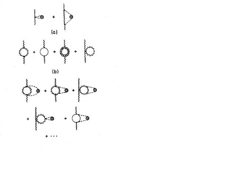
Figure 1: a) Calculation of the gluon self-energy in the condensate. The first term shows the origin of the gluon mass term in the mean-field approximation. The dashed line refers to a condensate gluon of zero momentum. In the second part of a) we show a contribution to the (irreducible) polarization tensor in the single (condensate) loop approximation. b) Diagrams which contribute to the polarization tensor in QCD. The wavy line is a gluon, the solid line is a quark, and the third diagram represents the gluon field. c) Some corrections to the diagrams of (b) due to the presence of a gluon condensate.

It is also useful to subtract the quantity given in Eq. (4.1) from the current and define

$$\hat{J}_{a}^{\mu}(k)=J_{a}^{\mu}(k)+m_{G}^{2}(g^{\mu\nu}-k^{\mu}k^{\nu}/k^{2})\mathcal{A}_{\nu}^{a}(k)$$ (4.6)

in momentum space. Then we have

$$\left[(k^{2}-m_{G}^{2})(g^{\mu\nu}-k^{\mu}k^{\nu}/k^{2})+\frac{1}{\lambda}k^{\mu}k^{\nu}\right]\,\mathcal{A}_{\nu}^{a}(k)=-\hat{J}_{a}^{\mu}(k).$$ (4.7)

We now write a first-order propagator as

$$i\mathcal{D}_{ab}^{(1)\mu\nu}(k)=-i\,\left[\frac{g^{\mu\nu}-k^{\mu}k^{\nu}/k^{2}}{k^{2}-m_{G}^{2}}+\lambda\frac{k^{\mu}k^{\nu}}{(k^{2}+i\epsilon)^{2}}\right]\delta_{ab},$$ (4.8)

and also write

$$i\mathcal{D}(k^{2})=i\mathcal{D}^{(1)}(k^{2})+i\mathcal{D}^{(1)}(k^{2})\left[\frac{i\Pi_{A}(k^{2})}{1-\frac{\Pi_{A}(k^{2})}{k^{2}-m_{G}^{2}}}\right]i\mathcal{D}^{(1)}(k^{2}),$$ (4.9)

where

$$\mathcal{D}^{(1)}(k^{2})=-[k^{2}-m_{G}^{2}]^{-1},$$ (4.10)

and

$$\mathcal{D}(k^{2})=-[k^{2}-m_{G}^{2}-\Pi_{A}(k^{2})]^{-1}.$$ (4.11)

Thus we see that, after absorbing the mass term in $\mathcal{D}_{\mu\nu}^{(1)}$, the quantity $\Pi_{A}(k^{2})$ is related to the time-ordered product of the $\hat{J}_{T,\mu}^{a}(x)$:

$$[g^{\mu\nu}-k^{\mu}k^{\nu}/k^{2}]\left[\frac{\Pi_{A}(k^{2})}{1-\frac{\Pi_{A}(k^{2})}{k^{2}-m_{G}^{2}}}\right]\delta_{ab}=i\,\int d^{4}x\,e^{ik\cdot x}<vac\mid T[\hat{J}_{T,a}^{\mu}(x)\hat{J}_{T,b}^{\nu}(0)]\mid vac>.$$ (4.12)

Equation (4.12) is a generalization of Eq. (2.18) and reflects the presence of a condensate in the QCD vacuum which makes the gluon massive. We also remark that, after gauge fixing, the theory with ghost fields has a form of gauge invariance - the BRST gauge symmetry. This symmetry allows one to derive the analog of the QCD Ward identities in QCD - the Slavnov-Taylor identities. (We note that the ghost condensate introduced in Ref. [26] is BRST invariant.)

V The gluon propagator and the Dielectric function in QCD

One is tempted to write the analog of Eq. (2.1) in the case of QCD. However, if there is a gluon condensate present, there is an essential modification to be considered. We recall that we found it useful to divide $A_{\mu}^{a}(x)$ into a condensate field, $\mathbb{A}^{a}_{\mu}(x)$, and a fluctuating field, $\mathcal{A}^{a}_{\mu}(x)$. (We made the assumption that the condensate field is in the zero-momentum mode and therefore, $\mathbb{A}_{a}^{\mu}(x)$ is independent of $x$.)

Thus, in coordinate space, we have

$$i\mathcal{D}_{\mu\nu}^{ab}(x,x^{\prime}) = <vac\mid T[A_{\mu}^{a}(x)A_{\nu}^{b}(x^{\prime})]\mid vac>$$ (5.1)

$$= <vac\mid\mathbb{A}_{\mu}^{a}\mathbb{A}_{\nu}^{b}\mid vac>+<vac\mid T[\mathcal{A}_{\mu}^{a}(x)\mathcal{A}_{\nu}^{b}(x^{\prime})]\mid vac>$$ (5.2)

$$= -\frac{g_{\mu\nu}}{4}\phi_{0}^{2}\frac{\delta_{ab}}{8}+<vac\mid T[\mathcal{A}_{\mu}^{a}(x)\mathcal{A}_{\nu}^{b}(x^{\prime})]\mid vac>.$$ (5.3)

Our expression for the gluon propagator in momentum space is then

$$i\mathcal{D}_{\mu\nu}^{ab}(k)=-\frac{g_{\mu\nu}}{4}\phi_{0}^{2}\frac{\delta_{ab}}{8}(2\pi)^{4}\delta^{(4)}(k)-i\,\left[\frac{(g_{\mu\nu}-k_{\mu}k_{\nu}/k^{2})}{k^{2}[1-\Pi_{1}(k^{2})]}+\lambda\frac{k_{\mu}k_{\nu}}{(k^{2}+i\epsilon)^{2}}\right].$$ (5.4)

We see the first characteristic difference when we compare Eq. (5.4) with Eq. (2.1), that is, the presence of a delta function. Whether such a term is present depends on whether or not one has a ground-state condensate in the zero-momentum mode.

We can define a QCD dielectric function:

$$\kappa(k^{2})=[1-\Pi_{1}(k^{2})].$$ (5.5)

As noted earlier, the Schwinger mechanism refers to the a fact that, if $\kappa(k^{2})$ has a pole at $k^{2}=0$, the gluon has a dynamical mass and the pole at $k^{2}=0$ in $\mathcal{D}_{\mu\nu}^{ab}(k)$ disappears. In an earlier work we found that $m_{G}^{2}=(9/32)g^{2}\phi_{0}^{2}$. As we will see in this work

$$\kappa(k^{2})=\left[1-\frac{m_{G}^{2}}{k^{2}}+\frac{4\eta^{2}}{k^{2}-m_{G}^{2}}\right]$$ (5.6)

where $\eta^{2}=(3/32)g^{2}\phi_{0}^{2}$. (Thus $m_{G}^{2}=3\eta^{2}$.) The result given in Eq. (5.6) follows from the calculation of the diagrams in Fig. 1 subject to the constraints required in the covariant formalism. The quantity $\kappa(k^{2})$ defined in Eq. (5.6) is shown in Fig. 2. It is interesting to note that if the Schwinger mechanism is operative, that is, if there is a pole in $\kappa(k^{2})$ at $k^{2}=0$, one needs an additional singularity to avoid having a zero in $\kappa(k^{2})$. Such a zero would imply that gluons could go on-mass-shell, a clearly unsatisfactory result. It is gratifying that at the next level of approximation (one condensate loop) one finds the necessary singular term that maintains the relation $\kappa(k^{2})\neq 0$.

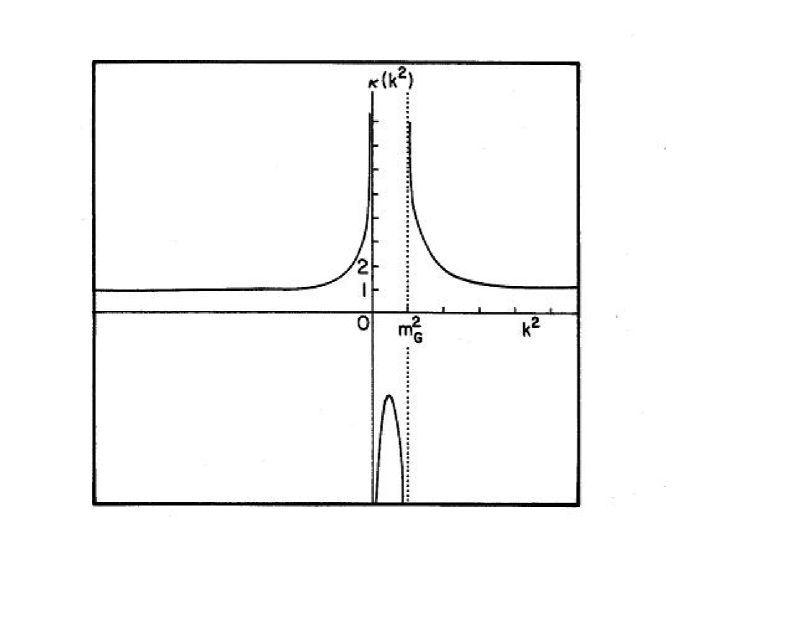
Figure 2: The dielectric constant $\kappa(k^{2})=[1-\frac{m_{G}^{2}}{k^{2}}+\frac{4\eta^{2}}{k^{2}-m_{G}^{2}}]$ is shown. The singularity at $k^{2}=0$ reflects the operation of the Schwinger mechanism [25]. (Here we see how the infrared singularities of the theory lead to nonpropagation of gluons in the QCD vacuum, a result which has long been conjectured to be true.)

We do not have all the terms contributing to $\kappa(k^{2})$. For example, there will be terms of order $g^{2}(\phi_{0}^{2}/k^{2})$ or $g^{2}\ln(\phi_{0}^{2}/\mid k^{2}\mid)$ in the deep Euclidean region. The origin of such terms may be seen in Fig. 1, where we have shown how the presence of the condensate can lead to (power) corrections to the asymptotic behavior of the polarization tensor in the region $k^{2}\rightarrow-\infty$.

We also note that the only way to form a small parameter in this model is to construct the ratio $[g^{2}\phi_{0}^{2}/(-k^{2})]$ which is small for large spacelike $k^{2}$. The nonperturbative analysis is clearly not an expansion in a small parameter. That is characteristic of nonperturbative approximations in general. Usually it is difficult to find a completely satisfactory organizational principle for a nonperturbative expansion. One that is extensively used is a loop expansion. The zero-loop or “tree-approximation” corresponds to the mean-field approximation. This approximation is used extensively in field theory and many-body physics. In our analysis the first term in Fig. 1a is identified as the “tree” or mean-field approximation. That approximation is sufficient to generate the gluon mass via the Schwinger mechanism. The second term in Fig. 1a may be thought of as a (condensate) one-loop correction to the mean-field approximation. It is, of course, interesting that we find nonpropagation of gluons already in the one-loop approximation. Increasing the number of condensate loops increases the number of factors of $g^{2}\phi_{0}^{2}$ which appear in the numerator of the terms which make up $\kappa(k^{2})$. That is, at the tree level, we obtain the $m_{G}^{2}/k^{2}$ term and at the one-loop level, we find the term $-4\eta^{2}/(k^{2}-m_{G}^{2})$.

We now wish to obtain the contribution to $\Pi^{\mu\nu}_{ab}(k)$ in the Landau gauge of the form

$$(g^{\mu\nu}-k^{\mu}k^{\nu}/k^{2})\,\left[\frac{-4\eta^{2}k^{2}}{k^{2}-m_{G}^{2}}\right]$$ (5.7)

displayed above. Various elements of our analysis are depicted in Figs. 3-5 which are taken from Ref. [27].

Combining the above result with Eq. (4.3), the mean-field plus the one (condensate) loop result for the polarization tensor is

$$\Pi_{\mu\nu}^{ab}(k)=\delta_{ab}(g_{\mu\nu}-k_{\mu}k_{\nu}/k^{2})\left[m_{G}^{2}-\frac{-4\eta^{2}k^{2}}{k^{2}-m_{G}^{2}}\right].$$ (5.8)

We had

$$\delta_{ab}(g^{\mu\nu}-k^{\mu}k^{\nu}/k^{2})\left[\frac{\Pi(k^{2})}{1-\frac{\Pi(k^{2})}{k^{2}-m_{G}^{2}}}\right]=i\int d^{4}x\,e^{ik\cdot x}<vac\mid T[\hat{J}_{T,a}^{\mu}(x)\hat{J}_{T,b}^{\nu}(0)]\mid vac>.$$ (5.9)

From our definition of $J_{\nu}^{a}(x)$, we find

$$J_{\nu}^{a}(x)=gf^{abc}[A_{b}^{\mu}(x)\partial_{\nu}A_{\mu}^{c}(x)-2A_{b}^{\mu}(x)\partial_{\mu}A_{\nu}^{c}(x)-A_{\nu}^{c}(x)\partial^{\mu}A_{\mu}^{b}(x)]$$ (5.10)

$$+g^{2}f^{abc}f^{a^{\prime}b^{\prime}c}[A_{\mu}^{b}(x)A_{b^{\prime}}^{\mu}(x)A_{\nu}^{a^{\prime}}(x)].$$

We insert

$$A_{\mu}^{a}(x)=\mathbb{A}_{\mu}^{a}(x)+\mathcal{A}^{a}_{\mu}(x)$$ (5.11)

into the last expression to obtain

$$J_{\nu}^{a}(x)=gf_{abc}[\mathbb{A}_{b}^{\mu}(x)\partial_{\nu}\mathcal{A}_{\mu}^{c}(x)-2\mathbb{A}_{b}^{\mu}(x)\partial_{\mu}\mathcal{A}_{\nu}^{c}(x)-\mathbb{A}_{\nu}^{c}(x)\partial^{\mu}\mathcal{A}_{\mu}^{b}(x)]$$ (5.12)

$$+gf_{abc}[\mathcal{A}_{b}^{\mu}(x)\partial_{\nu}\mathcal{A}_{\mu}^{c}(x)-2\mathcal{A}_{b}^{\mu}(x)\partial_{\mu}\mathcal{A}_{\nu}^{c}(x)-\mathcal{A}_{\nu}^{c}(x)\partial^{\mu}\mathcal{A}_{\mu}^{b}(x)]$$

$$+g^{2}f^{abc}f^{a^{\prime}b^{\prime}c}[\mathbb{A}_{\mu}^{b}(x)+\mathcal{A}_{\mu}^{b}(x)][\mathbb{A}^{\mu}_{b^{\prime}}(x)+\mathcal{A}^{\mu}_{b^{\prime}}(x)][\mathbb{A}_{\nu}^{a^{\prime}}(x)+\mathcal{A}_{\nu}^{a^{\prime}}(x)].$$

Since we are here working to order $(g^{2}\phi_{0}^{2})$, we will drop the last term of Eq. (5.12) at this point. (However, we note that it is responsible for the term proportional to $m_{G}^{2}$ in Eq. (5.8).) Thus, we may use the approximation

$$\bar{J}_{\nu}^{a}(x)\cong gf^{abc}[\mathbb{A}_{b}^{\mu}\partial_{\nu}\mathcal{A}_{\mu}^{c}(x)-2\mathbb{A}^{\mu}_{b}\partial_{\mu}\mathcal{A}_{\nu}^{c}(x)+\mathbb{A}_{\nu}^{b}\partial^{\mu}\mathcal{A}_{\mu}^{c}(x)]$$ (5.13)

for the calculation to be made here. (Note that, in the last term, we have interchanged $b$ and $c$ and changed the sign of that term.) We maintain the constraint

$$<\psi_{m}\mid\partial_{\mu}\bar{J}_{a}^{\mu}(x)\mid\psi_{n}>=0,$$ (5.14)

and implement that constraint by using only the conserved current, $\hat{J}_{T,\mu}^{a}(x)$, in our calculation. We can define the projection operator

$$\mathcal{P}_{\mu\nu}^{T}=g_{\mu\nu}-\partial_{\mu}\frac{1}{\Box}\partial_{\nu},$$ (5.15)

which in momentum space has the form

$$\mathcal{P}_{\mu\nu}^{T}=[g_{\mu\nu}-k_{\mu}k_{\nu}/k^{2}].$$ (5.16)

We have

$$\hat{J}_{T,\nu}^{a}(x)\equiv\mathcal{P}_{\nu\mu}^{T}J_{a}^{\mu}(x).$$ (5.17)

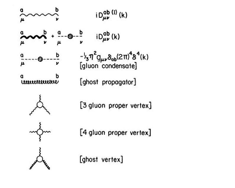
Figure 3: Diagrammatic representation of various elements of our model. Note that the dashed line contributes for $k_{\mu}=0$. (See Ref. [27] for further details.)

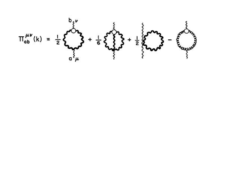
Figure 4: Diagrammatic representation of the equations determining the vacuum polarization tensor. (See Ref. [27].)

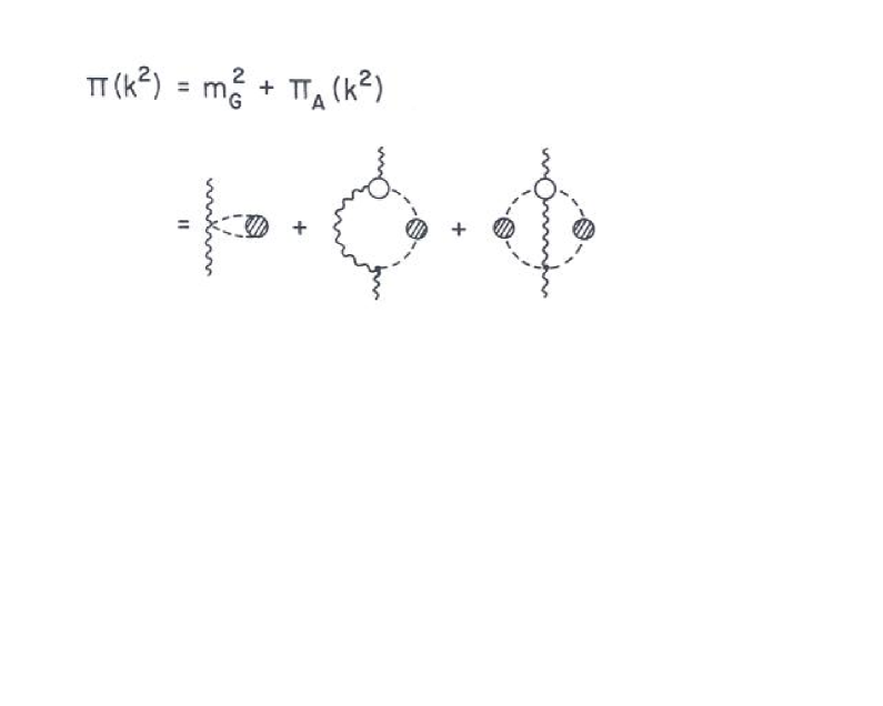
Figure 5: Diagrammatic representation of various elements of the polarization tensor used in this work. The first diagram on the right-hand side is responsible for the gluon mass term. [The vertex functions in the second two terms are to be expressed in terms of the full gluon propagator, $i\mathcal{D}_{\mu\nu}^{ab}(k)$.]

Thus, using Eq. (5.13), we find

$$\hat{J}_{T,\nu}^{a}(x)\simeq gf^{abc}[\mathbb{A}_{b}^{\rho}P_{\nu\mu}^{T}\partial^{\mu}\mathcal{A}_{\rho}^{c}(x)-2\mathbb{A}_{b}^{\rho}P_{\nu\mu}^{T}\partial_{\rho}\mathcal{A}_{c}^{\mu}(x)$$ (5.18)

$$+P^{T}_{\nu\mu}{\mathbb{A}_{b}^{\mu}\partial^{\rho}\mathcal{A}_{\rho}^{c}(x)}].$$

The first term in Eq. (5.18) is equal to zero. the last term in Eq. (5.18) can be dropped because of the constraint

$$<\psi_{n}\mid\partial_{\mu}\mathcal{A}_{c}^{\mu}(x)\mid\psi_{m}>=0.$$ (5.19)

To the order considered, we have

$$i\, < vac\mid T[\hat{J}_{T,a}^{\nu}(x)\hat{J}_{T,a^{\prime}}^{\nu^{\prime}}(x^{\prime})]\mid vac>\qquad\qquad\qquad\qquad\qquad\qquad\qquad\qquad\qquad\qquad\,\,\,\,\,\,\,\,\,$$ (5.20)

$$= i\,g^{2}f^{abc}f^{a^{\prime}b^{\prime}c}<vac\mid T\{-2\mathbb{A}_{\rho}^{b}P_{T}^{\nu\mu}\,\partial^{\rho}\mathcal{A}_{\mu}^{c}(x)\}\times\{-2\mathbb{A}_{\rho^{\prime}}^{b^{\prime}}P_{T}^{\nu^{\prime}\mu^{\prime}}\partial^{{}^{\prime}\rho^{\prime}}\mathcal{A}_{\mu^{\prime}}^{c^{\prime}}(x^{\prime})\}\mid vac>$$

$$= i\,g^{2}f^{abc}f^{a^{\prime}b^{\prime}c}<vac\mid\mathbb{A}_{\rho}^{b}\,\mathbb{A}_{\rho^{\prime}}^{b^{\prime}}\mid vac>$$

$$\times\{4P_{T}^{\nu\mu}\,P_{T}^{\nu^{\prime}\mu^{\prime}}\}<vac\mid T\{\partial^{\rho}\mathcal{A}_{\mu}^{c}(x)\,\partial^{\prime\rho^{\prime}}\mathcal{A}_{\mu^{\prime}}^{c^{\prime}}(x^{\prime})\}\mid vac>$$

$$= i\,g^{2}f^{abc}f^{a^{\prime}b^{\prime}c}\left[-\phi_{0}^{2}\frac{\delta_{bb^{\prime}}}{8}\frac{g_{\rho^{\prime}\rho}}{4}\right]\{4P_{T}^{\nu\mu}P_{T}^{\nu^{\prime}\mu^{\prime}}\}\,\partial^{\rho}\partial^{\prime\rho^{\prime}}\,[i\,\mathcal{D}_{\mu\mu^{\prime}}^{cc^{\prime}}(x,x^{\prime})].$$ (5.22)

We write

$$\mathcal{D}_{\mu^{\prime}\nu^{\prime}}^{cc^{\prime}}(x,x^{\prime})=\delta_{cc^{\prime}}\mathcal{D}_{\mu\nu^{\prime}}(x,x^{\prime}),$$ (5.23)

and find

$$i\,<vac\mid T[\hat{J}_{T,a}^{\nu}(x)\hat{J}_{T,a^{\prime}}^{\nu^{\prime}}(x^{\prime})]\mid vac>=\frac{3}{32}g^{2}\phi_{0}^{2}\,\delta_{aa^{\prime}}\,[\,4P_{T}^{\nu\mu}P_{T}^{\nu^{\prime}\mu^{\prime}}\partial_{\rho}\partial^{{}^{\prime}\rho}\,\mathcal{D}_{\mu\mu^{\prime}}(x,x^{\prime})].$$ (5.24)

Now introduce

$$\mathcal{D}_{\mu\mu^{\prime}}(k)=-\left[\frac{P^{T}_{\mu\mu^{\prime}}}{k^{2}-m_{G}^{2}-\Pi_{A}(k^{2})}+\frac{\lambda k_{\mu}k_{\mu^{\prime}}}{(k^{2}+i\epsilon)^{2}}\right],$$ (5.25)

and note that $\partial^{\rho}\partial^{{}^{\prime}}_{\rho}\rightarrow[ik^{\rho}][-ik_{\rho}]=k^{2}$.

Further, $P_{T}^{\nu\mu}P_{T}^{\nu^{\prime}\mu^{\prime}}P_{\mu\mu^{\prime}}^{T}=P_{T}^{\nu\nu^{\prime}}$, and therefore,

$$\delta_{aa^{\prime}}(g^{\nu\nu^{\prime}}-k^{\nu}k^{\nu^{\prime}}/k^{2})\left[\frac{\Pi_{A}(k^{2})}{1-\frac{\Pi_{A}(k^{2})}{k^{2}-m_{G}^{2}}}\right]=(g^{\nu\nu^{\prime}}-k^{\nu}k^{\nu^{\prime}}/k^{2})\left[\frac{-4\eta^{2}k^{2}}{k^{2}-m_{G}^{2}-\Pi(k^{2})}\right]\delta_{aa^{\prime}},$$ (5.26)

where $\eta^{2}=(3/32)g^{2}\phi_{0}^{2}$.

Thus

$$\frac{\Pi_{A}(k^{2})}{[1-\frac{\Pi_{A}(k^{2})}{k^{2}-m_{G}^{2}}]}=-\left[\frac{-4\eta^{2}k^{2}}{k^{2}-m_{G}^{2}-\Pi_{A}(k^{2})}\right],$$ (5.27)

which has the solution,

$$\Pi_{A}(k^{2})=\frac{-4\eta^{2}k^{2}}{k^{2}-m_{G}^{2}}.$$ (5.28)

Recall that

$$\Pi(k^{2})=m_{G}^{2}+\Pi_{A}(k^{2}),$$ (5.29)

which then yields Eq. (5.7).

One may ask how our result is related to the result of a diagrammatic analysis. It may be seen that the result given here is obtained if one calculates in the Landau gauge and adds a ghost condensate to maintain the transverse structure for $\Pi_{\mu\nu}(k)$. Indeed, Lavelle and Schaden [26] have used a ghost condensate to enforce the transverse nature of the nonperturbative part of $\Pi_{\mu\nu}(k)$. (Recall Eq. (2.26).) Their calculation is made in the deep-Euclidean region $(k^{2}\rightarrow-\infty)$. Therefore, we can compare our result with theirs, in the case a condensate $<:A^{2}:>$ is present, by taking $k^{2}\rightarrow-\infty$ in our result. From Eqs. (5.28) and (5.29) we have

$$\Pi(k^{2}) \longrightarrow m_{G}^{2}-\frac{4}{3}m_{G}^{2}\qquad k^{2}\rightarrow-\infty,$$ (5.30)

$$= -\frac{1}{3}m_{G}^{2},$$ (5.31)

$$= -\frac{3}{32}g^{2}(\tilde{\mu}^{2})\phi_{0}^{2},$$ (5.32)

which agrees with the result of Ref. [26], when that result is evaluated in the Landau gauge. (It is interesting to see how the sign of $\Pi(k^{2})$ changes as one passes from $k^{2}=0$ to $k^{2}=-\infty$.)

VI QCD lattice calculations and phenomenological forms for the Euclidean-space gluon propagator

The form we obtained for the propagator was

$$D^{\mu\nu}(k)=\left(g^{\mu\nu}-\frac{k^{\mu}k^{\nu}}{k^{2}}\right)D(k).$$ (6.1)

We now write

$$D(k)=\frac{Z_{1}}{k^{2}-m^{2}+\frac{4}{3}\frac{k^{2}m^{2}}{k^{2}-m^{2}}}.$$ (6.2)

Here $Z_{1}$ is a normalization parameter which we put equal to 3.82 so that we may obtain a continuous representation as we pass from Minkowski to Euclidean space. In Fig. 6 we show $D(k)$ with $m^{2}=0.25$ GeV². (We remark that $D(k)=0$ when $k^{2}=m^{2}$, $D(k)=-Z_{1}/m^{2}$ at $k^{2}=0$, and $D(k)\rightarrow Z_{1}/k^{2}$ for large $k^{2}$.) If we choce $Z_{1}=15.28m^{2}=3.82$ our result for the propagator will be continuous at $k^{2}=0$ when we consider both the Euclidean-space and Minkowski-space propagators.

Results for the gluon propagator obtained in a lattice simulation of QCD are given in Ref. [28]. In that work the authors also record several phenomenological forms. We reproduce these forms in the Appendix for ease of reference. Of these various forms we will make use of model A of Ref. [28] which has the form

$$D^{L}(k^{2})=Z\left[\frac{AM^{2\alpha}}{(k^{2}+M^{2})^{1+\alpha}}+\frac{1}{k^{2}+M^{2}}L(k^{2},M)\right],$$ (6.3)

with

$$L(k^{2},M)\equiv\left[\frac{1}{2}\ln(k^{2}+M^{2})(k^{-2}+M^{-2})\right]^{-d_{D}},$$ (6.4)

and $d_{D}=13/22$. The parameters used in Ref. [28] to provide a very good fit to the QCD lattice data are

$$Z=2.01^{+4}_{-5},$$ (6.5)

$$A=9.84^{+10}_{-86},$$ (6.6)

$$M=0.54^{+5}_{-5},$$ (6.7)

and

$$\alpha=2.17^{+4}_{-19}.$$ (6.8)

Note that $M$ in GeV units is $1.018$ GeV. Rather than work with the lattice data we will use Eqs. (6.3)-(6.8) when we compare our results with the lattice data. In Fig. 7 we show $k^{2}D^{L}(k)$ of Eq. (6.3) and in Fig. 8 we show $D^{L}(k)$. These functions are represented by the solid lines in Figs. 7 and 8. Note that Eq. (6.2) may be written in Euclidean space as

$$D_{E}(k)=-\frac{Z_{1}}{k^{2}_{E}+m^{2}-\frac{4}{3}\frac{k^{2}_{E}m^{2}}{k^{2}_{E}+m^{2}}}.$$ (6.9)

This form is useful for $k_{E}^{2}<1$ GeV² and we therefore consider various phenomenological forms which may be used to extend Eq. (6.9) so that we may attempt to fit the lattice result over a broader momentum range. To that end, we make use of Ref. [29]. The authors of that work define the Landau gauge gluon propagator as

$$<A^{a}_{\mu}(k)A^{a}_{\nu}(k^{\prime})>=V\delta(k+k^{\prime})\delta^{ab}\left(\delta_{\mu\nu}-\frac{k_{\mu}k_{\nu}}{k^{2}}\right)\frac{Z(k^{2})}{k^{2}},$$ (6.10)

with

$$Z(k^{2})=\omega\left(\frac{k^{2}}{\Lambda^{2}_{QCD}+k^{2}}\right)^{2\kappa}(\alpha(k^{2}))^{-\gamma},$$ (6.11)

and $\gamma=-13/22$. (We do not ascribe any particular significance to Eq. (6.11). We use Eq. (6.11) as a phenomenological form which could be replaced by a form which provides a better fit to the data within the context of our model at some future time. We believe Eq. (6.11) is useful, since it is a simple matter to remove the first term of that equation and introduce a propagator that has the small $k^{2}$ behavior of our model.)

The authors of Ref. [29] introduce two choices for $\alpha(k^{2})$ of Eq. (6.11). We use their form for $\alpha_{2}(k^{2})$:

$$\alpha_{2}(k^{2})=\frac{\alpha(0)}{\ln\left[e+a_{1}\left(\frac{k^{2}}{\Lambda^{2}_{QCD}}\right)^{a_{2}}\right]}.$$ (6.12)

In their analysis they put $\kappa=0.5314$, $\Lambda_{QCD}=354$ MeV, $\alpha(0)=2.74$, $a_{1}=0.0065$ and $a_{2}=2.40$. (Here, we have not recorded the uncertainties in these values which are given in Table 2 of Ref. [29].) As we proceed, we will change these values somewhat. As a first step we remove the first factor in Eq. (6.11) and write

$$Z(k^{2})=Z_{2}(\alpha_{2}(k^{2}))^{-\gamma}.$$ (6.13)

We now use $a_{1}=0.0080$ and $a_{2}=2.10$ rather than the values given above. In Fig. 9 we show $(\alpha_{2}(k))^{13/22}$ as a function of $k$, using our modified values of $a_{1}$ and $a_{2}$.

We now define

$$D_{E}(k_{E})=-\frac{Z_{2}(\alpha(k^{2}))^{-\gamma}}{k_{E}^{2}+m^{2}-\frac{4}{3}\frac{k_{E}^{2}m^{2}}{k_{E}^{2}+m^{2}}}.$$ (6.14)

The function $-k^{2}D_{E}(k_{E})$ is shown in Fig. 7 as a dotted line. In this calculation we have put $Z_{2}=2.11$. We find a good representation of the lattice result for $k_{E}<2$ GeV,

In Fig. 8 we compare $D_{E}(k_{E})$ with the result of the lattice calculation which is represented by the solid line. In Fig. 10 we combine our results in Minkowski and Euclidean space and show the values of $k^{2}D(k^{2})$ for both positive and negative $k^{2}$ values. For positive $k^{2}$ we use $D(k)$ of Eq. (6.2) and for negative values of $k^{2}$ we use $D_{E}(k_{E}^{2})$ of Eq. (6.14). Equality of these functions at $k^{2}=0$ implies $Z_{1}=Z_{2}(\alpha(0))^{13/22}$, or $Z_{1}=1.81Z_{2}$. (In our work we have used $Z_{1}=3.82$ and $Z_{2}=2.11$. See Eqs. (6.2) and (6.14).) In Fig. 11 we show $D(k^{2})$ rather than $k^{2}D(k^{2})$, which was shown in Fig. 10.

Figure 6: The function $D(k^{2})$ of Eq. (6.2) is shown in Minkowski space. The value for large $k^{2}$ is given by $Z_{1}/k^{2}$ with $Z_{1}=3.87$. Here $m=0.50$ GeV.

Figure 7: The function $-k_{E}^{2}D_{E}(k)$ is shown. The solid line represents the QCD lattice data, while the dotted line represents $-k^{2}_{E}D_{E}(k)$ in the case that $D_{E}(k)$ is given in Eq. (6.14).

Figure 8: The function $-D_{E}(k)$ is shown. The solid line represents the QCD lattice data, while the dotted line represents $-D_{E}(k)$ of Eq. (6.14). [See Fig. 7.]

Figure 9: The function $(\alpha_{2}(k))^{13/22}$ is shown. [See Eq. (6.12).] Note that $(\alpha_{2}(0))^{13/22}=1.81$.

Figure 10: For $k^{2}>0$ the solid line represents $k^{2}D(k^{2})$ with $D(k^{2})$ given by Eq. (6.2). Here, $Z_{1}=3.82$. For $k^{2}<0$ we show $k^{2}D_{E}(k^{2})$, where $D_{E}(k^{2}_{E})$ is given by Eq. (6.14) with $Z_{2}=2.11$.

Figure 11: Same as Fig. 10 except that $D(k^{2})$ is shown.

VII discussion

In this work we have developed nonperturbative approximations for the description of the gluon condensate and have calculated the form of the gluon propagator. The approximation used may be thought of as a condensate-loop expansion. Since the condensate is assumed to be in the zero-momentum mode, the loop expansion does not require loop integrals, but leads to algebraic relations. Our results are obtained in the Landau gauge. (Note that ghosts are introduced to maintain the transverse character of $\Pi_{\mu\nu}(k)$ in Ref. [26].) We are able to make some contact with lattice calculations of the gluon propagator, which are made in the Landau gauge. We find that our value for the dynamical gluon mass, $m_{G}\simeq$ 600 MeV, is in accord with the results of recent lattice calculations. We have also seen that our results agree with those of Lavelle and Schaden, if one evaluates our propagators in the deep-Euclidean region $(k^{2}\rightarrow-\infty)$ [26].

In our work, confinement of quarks and gluons and chiral symmetry breaking are related to a single condensate order parameter $(g^{2}\phi_{0}^{2})$. This result is consistent with the fact that in lattice simulations of QCD, deconfinement and chiral symmetry restoration take place at the same temperature. In this connection, we note that there is no threshold value of $(g^{2}\phi_{0}^{2})$. For any finite value of this parameter, we find chiral symmetry breaking and nonpropagation of quarks [30] and gluons.

In this work we have provided a representation of the gluon propagator in both Euclidean and Minkowski space. The Minkowski-space propagator has only complex poles and that implies that the gluon is a nonpropagating mode in the QCD vacuum. Our analysis takes into account the important condensate $<A_{a}^{\mu}A_{\mu}^{a}>$ which is responsible for mass generation for the gluon. Our work has some relation to that of Cornwall [31] who obtained a gluon mass of $500\pm 200$ MeV in his analysis. Cornwall also suggested that “quark confinement arises from a vertex condensate supported by a mass gap.”

In recent work, Gracey obtained a pole mass of the gluon of $2.13\Lambda_{\overline{MS}}$ in a two-loop renormalization scheme [32]. If we put $\Lambda_{\overline{MS}}=250$ MeV, the mass obtained at two-loop order in Ref. [32] is $532$ MeV, which is close to the value of $500$ MeV used in the present work. (We remark that in Ref. [22] we obtained a gluon mass of $530$ MeV, if we made use of Eq. (3.18) of that reference, which includes the effect of including various exchange terms in our analysis of the relevant matrix elements.)

Appendix A

For ease of reference we record various semi-phenomenological forms which are meant to represent the Euclidean-space gluon propagator.

Gribov [33]:

$$D^{L}(k^{2})=\frac{Zk^{2}}{k^{4}+M^{4}}L(k^{2},M).$$ (A1)

Stingl [34]:

$$D^{L}(k^{2})=\frac{Zk^{2}}{k^{4}+2A^{2}k^{2}+M^{4}}L(k^{2},M).$$ (A2)

Marenzoni et al. [35]:

$$D^{L}(k^{2})=\frac{Z}{(k^{2})^{1+\alpha}+M^{2}}.$$ (A3)

Cornwall I [31]:

$$D^{L}(k^{2})=Z\left[[k^{2}+M^{2}(k^{2})]\ln\left(\frac{k^{2}+4M^{2}(k^{2})}{\Lambda^{2}}\right)\right]^{-1},$$ (A4)

where

$$M(k^{2})=M\left[\frac{\ln\left(\frac{k^{2}+4M^{2}}{\Lambda^{2}}\right)}{\ln\left(\frac{4M^{2}}{\Lambda^{2}}\right)}\right]^{-6/11}.$$ (A5)

Cornwall II [36]:

$$D^{L}(k^{2})=Z\left[[k^{2}+M^{2}]\ln\left(\frac{k^{2}+4M^{2}}{\Lambda^{2}}\right)\right]^{-1}.$$ (A6)

Cornwall III [36]:

$$D^{L}(k^{2})=\frac{Z}{k^{2}+Ak^{2}\ln\left(\frac{k^{2}}{M^{2}}\right)+M^{2}}.$$ (A7)

Model A [28]:

$$D^{L}(k^{2})=Z\left[\frac{AM^{2\alpha}}{(k^{2}+M^{2})^{1+\alpha}}+\frac{1}{k^{2}+M^{2}}L(k^{2},M)\right].$$ (A8)

The parameters for model A are given in Eqs. (6.5)-(6.7).
Model B [28]:

$$D^{L}(k^{2})=Z\left[\frac{AM^{2\alpha}}{(k^{2})^{1+\alpha}+(M^{2})^{1+\alpha}}+\frac{1}{k^{2}+M^{2}}L(k^{2},M)\right].$$ (A9)

Model C [28]:

$$D^{L}(k^{2})=Z\left[\frac{A}{M^{2}}e^{-(k^{2}/M^{2})^{\alpha}}+\frac{1}{k^{2}+M^{2}}L(k^{2},M)\right].$$ (A10)

References

(1)Ph. Boucaud, A. Le Yaouanc, J. P. Leroy, J.
Micheli, O. Pne and J. Rodriguez-Quintero, Phys. Rev. D 63,
114003 (2001).
(2)Ph. Boucaud, A. Le Yaouanc, J. P. Leroy, J.
Micheli, O. Pne and J. Rodriguez-Quintero, Phys. Lett. B 493,
315 (2000).
(3)E. R. Arriola, P. O. Bowman, and W. Broniowski,
hep-ph/0408309, v3.
(4)Ph. Boucaud, J. P. Leroy, A Le Yaouanc, J. Micheli, O. Pne, F. DeSoto, A. Donini, H. Moutarde and
J. Rodriguez-Quintero, Phys. Rev. D 66, 034504 (2002).
(5) B. M. Gripaios, Phys. Lett. B 558, 250
(2003).
(6)K.-I. Kondo, Phys. Lett. B 572,
210(2003).
(7)K.-I. Kondo, Phys. Lett. B 514,
335(2001).
(8)A. A. Slavov, hep-th/0407194.
(9) L. Stodolsky, Pierre van Baal and V. I. Zakharov,
Phys. Lett. B 552, 214(2002).
(10)F. V. Gubarev, L. Stodolsky, and V. I. Zakharov, Phys. Rev.
Lett. 86, 2220 (2001).
(11)F. V. Gubarev, V. I. Zakharov, Phys. Lett. B 501, 28(2001).
(12)J. A. Gracey, Phys. Lett. B 552, 101 (2003). See also D. Dudal, H. Verschelde and S. P. Sorella, Phys.
Lett. B 555, 126 (2003).
(13)D. Dudal, H. Verschelde, R. E. Browne and J. A. Gracey, Phys.
Lett. B 562, 87(2003).
(14)D. Dudal, H. Verschelde, V. E. R. Lemes, M. S.
Sarandy, R. F. Sobreiro, S. P. Sorella, M. Picariello, A.
Vicini and J. A. Gracey, hep-th/0308153.
(15) H. Verschelde, K. Knecht, K. Van Acoleyen and V. Vanderkelen, Phys. Lett. B 516, 307(2001).
(16)D. Dudal, H. Verschelde, V. E. R. Lemes, M. S.
Sarandy, R. F. Sobreiro, S. P. Sorella and J. A. Gracey, Phys.
Lett. B 574, 325(2003).
(17)D. Dudal, H. Verschelde, J. A. Gracey, V. E. R. Lemes, M. S.
Sarandy, R. F. Sobreiro and S. P. Sorella, JHEP 0401,
044(2004); hep-th/0311194, v3.
(18)R. E. Browne and J. A. Gracey, JHEP 0311,
029(2003); hep-th/0306200.
(19)D. Dudal, J. A. Gracey, V. E. R. Lemes, R. F. Sobreiro, S. P.
Sorella and H. Verschelde, hep-th/0409254.
(20) B. L. Ioffe, Phys. Atom. Nucl. 66, 30 (2003)
(21) B. L. Ioffe and K. N. Zyablyuk, Eur. Phys. J. C 27,
229 (2003)
(22)L. S. Celenza and C. M. Shakin, Phys. Rev. D
34, 1591(1986)
(23)M. A. Shifman, A. I. Vainstem and V. I.
Zakharov, Nucl. Phys. B 147, 385 (1979); B
147, 448(1979); B 147, 519(1979).
(24)L. S. Celenza, Chueng-Ryong Ji and C. M. Shakin, Phys. Rev. D
36, 895(1987)
(25)J. Schwinger, Phys. Rev. 125, 397(1962).
(26)M. J. Lavelle and M. Schaden, Phys. Lett.
208, 297(1988).
(27)E. J. Eichten and G. L. Feinberg, Phys. Rev. D
10, 3254(1974).
(28)D. B. Leinweber, J. I. Skullerud, A. G. Williams
and C. Parrinello, Phys. Rev. D 60, 094507(1999).
(29)O. Oliveira and P. J. Silva, hep-lat/0410048.
(30) Xiangdong Li and C. M. Shakin, Phys. Rev. D 70,
114011 (2004)
(31)J. Cornwall, Phys. Rev. D 26, 1453(1982).
(32)J. A. Gracey, hep-ph/0411169.
(33)V. N. Gribov, Nucl. Phys. B 139,
19(1978).
(34)M. Stingl, Phys. Rev. D 34, 3863(1986);
36, 651(1987).
(35)P. Merenzoni, G. Martinelli and N. Stella, Nucl.
Phys. B 455, 339(1995); P. Marenzoni, G. Martinelli, N.
Stella and M. Testa, Phys. Lett. B 318, 511(1993).
(36)J. Cornwall (private communication to the authors
of Ref.[28]).