Quark Effects in the Gluon Condensate Contribution to the Scalar Glueball Correlation Function

Abstract

One-loop quark contributions to the dimension-four gluon condensate term in the operator product expansion (OPE) of the scalar glueball correlation function are calculated in the $\overline{\text{MS}}$ scheme in the chiral limit of $n_{\text{f}}$ quark flavours. The presence of quark effects is shown not to alter the cancellation of infrared (IR) singularities in the gluon condensate OPE coefficients. The dimension-four gluonic condensate term represents the leading power corrections to the scalar glueball correlator and, therein, the one-loop logarithmic contributions provide the most important condensate contribution to those QCD sum-rules independent of the low-energy theorem (the subtracted sum-rules).

The QCD correlation function of scalar gluonic currents

$$\Pi\left(q^{2}\right)=\mathrm{i}\int\!\mathrm{d}^{D}\!x\;\mathrm{e}^{\mathrm{i}q\cdot x}\langle 0|\mathcal{T}J(x)J(0)|0\rangle,$$ (1)

$$J(x)=\alpha G^{a}_{\mu\nu}(x)G^{a\mu\nu}(x)\equiv\alpha G^{2}(x),$$ (2)

is used to study the properties of scalar gluonium via QCD sum-rule techniques [1, 2]. The current $J(x)$ is the lowest-order version of the operator $\beta(\alpha)G^{2}(x)$, which is renormalization-group invariant for chiral quarks [3, 4]. As first noted in [5, 6], the one-loop gluon condensate contribution to (1)

$$\left[a_{0}+b_{0}\frac{\alpha}{\mathrm{\pi}}+b_{1}\frac{\alpha}{\mathrm{\pi}}\log\left(\frac{-q^{2}}{\nu^{2}}\right)\right]\left\langle\alpha G^{2}\right\rangle,$$ (3)

where $\{a_{0},\,b_{0},\,b_{1}\}$ are numerical coefficients (see (26)–(28) below), represents the leading condensate contribution to those sum-rules independent of the low-energy theorem [7], and so provide important non-perturbative effects within sum-rule analyses of scalar glueballs.

The one-loop coefficients $b_{0}$ and $b_{1}$ were evaluated in [5] in the absence of quark effects (i.e. the $n_{\text{f}}=0$ limit). As these $n_{\text{f}}=0$ gluon condensate effects have been used in a number of sum-rule analyses where the effects of three quark flavours have been included in the perturbative part [2], it is necessary to extend the results of [5] to enable self-consistent sum-rule analyses in the presence of $n_{\text{f}}$ chiral quarks.

Since the gluonic current (2) is gauge invariant, the operator product expansion (OPE) of the corresponding two-point operator contains only those local operators which are gauge invariant, equations of motion, or BRS variations [10]; hence, for massless quarks, the relevant OPE is given by

$$\mathrm{i}\int\!\mathrm{d}^{D}\!x\;\mathrm{e}^{\mathrm{i}q\cdot x}\mathcal{T}G^{2}(x)G^{2}(0)\\ =\mathcal{I}(q^{2})+\mathcal{C}(q^{2}):\!G^{2}(0)\!:+\mathcal{D}(q^{2})q^{\sigma}q^{\lambda}\left[:\!G^{a}_{\ \mu\sigma}(0)G^{a\mu}_{\ \ \lambda}(0)\!:-\frac{1}{D}g_{\sigma\lambda}:\!G^{2}(0)\!:\right]\\ +\text{equation of motion \& BRS invariant operators}+\text{higher dimensional operators}$$ (4)

where $\mathcal{I}(q^{2}),\,\mathcal{C}(q^{2}),\,\mathcal{D}(q^{2})$ are the Wilson (OPE) coefficients and where the two colons indicate normal ordering. For notational convenience, the normal ordering symbol and the spacetime argument will subsequently be omitted from the right-hand side of (4).

The scalar gluonic correlator (1) is obtained from (4) through multiplication by $\alpha^{2}$ followed by a vacuum expectation value (VEV). Physical matrix elements of the equation of motion and BRS invariant operators vanish, as does the VEV of the gluonic operator proportional to $\mathcal{D}(q^{2})$. Therefore, up to dimension four operators, the sole contributions to (1) stem from $\mathcal{I}(q^{2})$ (perturbation theory) and $\mathcal{C}(q^{2})$. This article is concerned with the latter.

As in [5], the nonzero momentum insertion technique (NZI method) [8, 9] is employed to compute OPE coefficients. This method sandwiches the OPE between two external single gluon states with momenta $k_{1}\neq k_{2}$, permitting the simple separation of (non-physical) operators whose VEV is zero (i.e. BRS invariants and equations of motion) from the physical operator $G^{2}$, thus simplifying the operator-mixing effects originating from the renormalization of composite operators [4]. The NZI method also facilitates the analysis of infrared aspects of the OPE, since the nonzero difference between the external gluon momenta $s=\left(k_{1}-k_{2}\right)^{2}$ provides an infrared regulator. As shown in [9] for the $n_{\text{f}}=0$ case, all infrared logarithms (i.e. $\log(s)$, $\log{\left(k_{1}^{2}\right)}$, and $\log{\left(k_{2}^{2}\right)}$) cancel in the calculation of the OPE coefficients. This then allows the use of on-shell external gluon states

$$|n\rangle\equiv|\epsilon_{n},\,k_{n},\,c_{n}\rangle,~{}\epsilon_{n}\cdot k_{n}=k_{n}^{2}=0$$ (5)

to sandwich the OPE, immediately eliminating all non-physical operators. The colour index $c_{n}$ associated with the gluon states (5) is included for completeness, but only leads to trivial overall colour factors when taking matrix elements of colour singlet objects such as (4). As will be discussed below, the IR cancellation in the OPE coefficients is not altered by the inclusion of quarks, and hence these simplifications can be applied even in the presence of chiral quarks.

Sandwiching (4) between on-shell gluon states yields

$$\mathrm{i}\int\!\mathrm{d}^{D}\!x\;\mathrm{e}^{\mathrm{i}q\cdot x}\langle 1|\mathcal{T}G^{2}(x)G^{2}(0)|2\rangle=\mathcal{C}(q^{2})\langle 1|G^{2}|2\rangle+\mathcal{D}(q^{2})q^{\sigma}q^{\lambda}\langle 1|G^{a}_{\ \mu\sigma}G^{a\mu}_{\ \ \lambda}-\frac{1}{D}g_{\sigma\lambda}G^{2}|2\rangle\\ +\text{contributions from higher dimension ($d>4$) operators},$$ (6)

where the matrix elements of all non-physical operators have been eliminated through the use of on-shell external gluon states. To simulate the effects of a VEV, the direction averaging operator $\int\!\mathrm{d}\hat{q}$ which, for example, leads to the identity

$$\int\!\mathrm{d}\hat{q}\;q_{\alpha}q_{\beta}f(q^{2})=\frac{1}{D}q^{2}g_{\alpha\beta}f(q^{2}),$$ (7)

is applied to (6). Consequently, the term proportional to $\mathcal{D}(q^{2})$ is annihilated (as in the VEV). In addition, it should be noted that $\langle 1|G^{2}|2\rangle=\mathcal{O}(k_{1,2}^{2})$ whereas the remaining terms on the right-hand side of (6) go like $\mathcal{O}(k_{1,2}^{4})$. In this way, contributions relevant to the computation of $\mathcal{C}(q^{2})$ are easily identified. Therefore, Eq. (6) implies

$$\mathrm{i}\int\!\mathrm{d}\hat{q}\,\mathrm{d}^{D}\!x\;\mathrm{e}^{\mathrm{i}q\cdot x}\langle 1|\mathcal{T}G^{2}(x)G^{2}(0)|2\rangle=\mathcal{C}(q^{2})\langle 1|G^{2}|2\rangle+\mathcal{O}(k_{1,2}^{4}).$$ (8)

Thus, at leading and next-to-leading order (respectively denoted by the $(0)$ and $(1)$ superscripts in what follows) in the bare fields, we have the set of equations

$$\mathrm{i}\int\!\mathrm{d}\hat{q}\,\mathrm{d}^{D}\!x\;\mathrm{e}^{\mathrm{i}q\cdot x}\langle 1|\mathcal{T}G_{B}^{2}(x)G_{B}^{2}(0)|2\rangle^{(0)} =\mathcal{C}^{(0)}(q^{2})\langle 1|G_{B}^{2}|2\rangle^{(0)}+\mathcal{O}(k_{1,2}^{4}),$$ (9)

$$\mathrm{i}\int\!\mathrm{d}\hat{q}\,\mathrm{d}^{D}\!x\;\mathrm{e}^{\mathrm{i}q\cdot x}\langle 1|\mathcal{T}G_{B}^{2}(x)G_{B}^{2}(0)|2\rangle^{(1)} =\mathcal{C}^{(0)}(q^{2})\langle 1|G_{B}^{2}|2\rangle^{(1)}+\mathcal{C}^{(1)}(q^{2})\langle 1|G_{B}^{2}|2\rangle^{(0)}+\mathcal{O}(k_{1,2}^{4}),$$ (10)

where the subscript $B$ denotes a perturbative expansion in terms of bare (unrenormalized) quantities.

Consider first (9) which, in terms of Feynman diagrams, is given schematically by

$$\mathrm{i}\int\!\mathrm{d}\hat{q}\left\{\raisebox{-0.5pt}{\includegraphics[scale={0.5}]{Glue1.eps}}+{\rm crossed~{}diagram}\right\}=\mathcal{C}^{(0)}(q^{2})\left\{\raisebox{-0.5pt}{\includegraphics[scale={0.5}]{Glue2.eps}}\right\}+\mathcal{O}(k_{1,2}^{4}).$$ (11)

which implies

$$\frac{64}{D}\delta^{c_{1}c_{2}}\left[(k_{1}\cdot k_{2})(\epsilon_{1}\cdot\epsilon_{2})-(k_{1}\cdot\epsilon_{2})(k_{2}\cdot\epsilon_{1})\right]+\mathcal{O}(k_{1,2}^{4})\\ =4\mathcal{C}^{(0)}(q^{2})\delta^{c_{1}c_{2}}\left[(k_{1}\cdot k_{2})(\epsilon_{1}\cdot\epsilon_{2})-(k_{1}\cdot\epsilon_{2})(k_{2}\cdot\epsilon_{1})\right]+\mathcal{O}(k_{1,2}^{4}).$$ (12)

Therefore

$$\mathcal{C}^{(0)}(q^{2})=\frac{16}{D},$$ (13)

and we note that, at leading order, $\mathcal{C}(q^{2})$ is unaffected by the inclusion of chiral quarks. The spacetime dimension $D$ must be kept arbitrary until later stages of the calculations.

Quark contributions to $\mathcal{C}(q^{2})$ do, however, show up at next-to-leading order, but only through that contribution to the left-hand side of (10) stemming from the diagram (and its crossed counterpart) depicted in Figure 1. This diagram does not generate any IR singularities in the OPE analysis since the external gluon momenta regulate the IR behaviour associated with the quark loop. Hence, the conclusion that all IR singularities cancel in the calculation of the gluon condensate OPE coefficient [5] is upheld in the presence of chiral quarks. As in [5], this cancellation then permits an expansion in the external gluon momenta prior to evaluating Feynman integrals (as opposed to an expansion after evaluating Feynman integrals used to explicitly show the IR-cancellation).

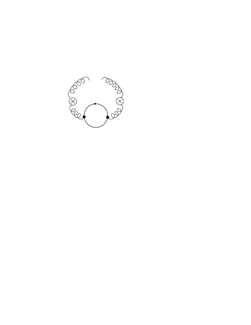
Figure 1: Feynman diagram containing quark effects contributing to the amplitude on the left-hand side of (10).

Having justified an expansion in external momenta prior to evaluating Feynman integrals, it immediately follows that

$$\langle 1|G_{B}^{2}|2\rangle^{(1)} =\raisebox{-0.5pt}{\includegraphics[scale={0.6}]{Glue3.eps}}+\raisebox{-0.5pt}{\includegraphics[scale={0.6}]{Glue4.eps}}$$

$$\quad+\raisebox{-0.5pt}{\includegraphics[scale={0.6}]{Glue5.eps}}+\raisebox{-0.5pt}{\includegraphics[scale={0.6}]{Glue6.eps}}$$

$$=\mathcal{O}(k_{1,2}^{4}),$$ (14)

as a consequence of the resulting massless tadpole integrals, and hence (10) can be simplified to

$$\mathrm{i}\int\!\mathrm{d}\hat{q}\,\mathrm{d}^{D}\!x\;\mathrm{e}^{\mathrm{i}q\cdot x}\langle 1|\mathcal{T}G_{B}^{2}(x)G_{B}^{2}(0)|2\rangle^{(1)}=4\delta^{c_{1}c_{2}}\mathcal{C}^{(1)}(q^{2})\left[(k_{1}\cdot k_{2})(\epsilon_{1}\cdot\epsilon_{2})-(k_{1}\cdot\epsilon_{2})(k_{2}\cdot\epsilon_{1})\right]+\mathcal{O}(k_{1,2}^{4}).$$ (15)

Calculation of the left-hand side of (15) constitutes a sizeable project. Fortunately, the vast majority of the required work has already been completed in [5]. Therein, all contributions within the framework of purely gluonic QCD were considered. Therefore, to extend the result to include chiral quarks, only those additional diagrams which admit internal quark loops need to be summed. As previously noted, at next-to-leading order, there are, in fact, only two such diagrams. Thus,

$$\mathrm{i}\int\!\mathrm{d}\hat{q}\,\mathrm{d}^{D}\!x\;\mathrm{e}^{\mathrm{i}q\cdot x}\langle 1|\mathcal{T}G_{B}^{2}(x)G_{B}^{2}(0)|2\rangle^{(1)}$$

$$\quad=4\delta^{c_{1}c_{2}}\frac{\alpha_{{}_{B}}}{\pi}\left\{-11\left[\frac{1}{\hat{\varepsilon}}+\log\left(\frac{-q^{2}}{\nu^{2}}\right)\right]+\frac{131}{6}\right\}\left[(k_{1}\cdot k_{2})(\epsilon_{1}\cdot\epsilon_{2})-(k_{1}\cdot\epsilon_{2})(k_{2}\cdot\epsilon_{1})\right]+\mathcal{O}(k_{1,2}^{4})$$

$$\qquad+\mathrm{i}\int\mathrm{d}\hat{q}\left\{\raisebox{-0.5pt}{\includegraphics[scale={0.5}]{Glue7.eps}}+{\rm crossed~{}diagram}\right\}$$ (16)

$$\quad=4\delta^{c_{1}c_{2}}\frac{\alpha_{{}_{B}}}{\pi}\left\{\left(\frac{2}{3}n_{\text{f}}-11\right)\left[\frac{1}{\hat{\varepsilon}}+\log\left(\frac{-q^{2}}{\nu^{2}}\right)\right]+\left(\frac{131}{6}-\frac{13}{9}n_{\text{f}}\right)\right\}$$ (17)

$$\qquad\times\left[(k_{1}\cdot k_{2})(\epsilon_{1}\cdot\epsilon_{2})-(k_{1}\cdot\epsilon_{2})(k_{2}\cdot\epsilon_{1})\right]+\mathcal{O}(k_{1,2}^{4})$$ (18)

where $D=4+2\varepsilon$, $\frac{1}{\hat{\varepsilon}}=\frac{1}{\varepsilon}-\gamma_{{}_{E}}+\ln(4\pi)$ and where the first term on the right-hand side of (16) is the purely gluonic contribution calculated in [5]. Together, Eqs. (15) and (18) imply that

$$\mathcal{C}^{(1)}(q^{2})=\frac{\alpha_{{}_{B}}}{\pi}\left\{\left(\frac{2}{3}n_{\text{f}}-11\right)\left[\frac{1}{\hat{\varepsilon}}+\log\left(\frac{-q^{2}}{\nu^{2}}\right)\right]+\left(\frac{131}{6}-\frac{13}{9}n_{\text{f}}\right)\right\}.$$ (19)

Lastly, recalling (2) and using (13) and (19), we find

$$\mathrm{i}\int\!\mathrm{d}^{D}\!x\;\mathrm{e}^{\mathrm{i}q\cdot x}\langle 0|\mathcal{T}J_{B}(x)J_{B}(0)|0\rangle$$

$$\quad=\alpha_{{}_{B}}\left[\mathcal{C}^{(0)}(q^{2})+\mathcal{C}^{(1)}(q^{2})\right]\langle\alpha_{{}_{B}}G^{2}_{B}\rangle+\cdots$$

$$\quad=4\alpha_{{}_{B}}\left\{\frac{4}{D}+\frac{\alpha_{{}_{B}}}{\pi}\left[\left(\frac{n_{\text{f}}}{6}-\frac{11}{4}\right)\left(\frac{1}{\hat{\varepsilon}}+\log\left(\frac{-q^{2}}{\nu^{2}}\right)\right)+\left(\frac{131}{24}-\frac{13}{36}n_{\text{f}}\right)\right]\right\}\langle\alpha_{{}_{B}}G^{2}_{B}\rangle+\cdots$$ (20)

where the dots represent contributions to the scalar gluonic correlator arising from operators of dimension other than four.

Eq. (20) is expressed in terms of bare quantities and so must be renormalized. Renormalization of composite operators is, of course, complicated by operator mixing [4]. Briefly, renormalized versions (no subscript) of $\alpha$ and $G^{2}$ are defined as

$$\alpha=Z^{-1}_{\alpha}\alpha_{{}_{B}},$$ (21)

$$G^{2}=Z_{G^{2}}G^{2}_{B}+\cdots$$ (22)

where the dots in (22) represent contributions from equation of motion and BRS invariant operators. Vacuum expectation values of these omitted operators vanish and so they do not contribute to the calculation at hand; only $Z_{G^{2}}$ is actually required. In the $\overline{\text{MS}}$ scheme the renormalization constant is [4]

$$Z_{G^{2}}=Z_{\alpha}=1+\frac{\alpha}{\mathrm{\pi}}\left(\frac{11}{4}-\frac{n_{\text{f}}}{6}\right)\frac{1}{\hat{\varepsilon}};$$ (23)

thus, $\alpha G^{2}$ is renormalization-group invariant at next-to-leading order. An analysis of the renormalization of $G^{2}$ using the NZI method is presented in [6], where $Z_{G^{2}}$ is easily distinguished from similarly defined renormalization constants corresponding to the omitted operators; hence $Z_{G^{2}}$ can be determined by consideration of only a single amplitude: $\langle 1|G^{2}_{B}|2\rangle$. Noting that

$$\frac{4}{D}=1-\frac{\varepsilon}{2},$$ (24)

substitution of (21) and (22) into (20) yields the following result in the $\overline{\text{MS}}$ scheme:

$$\mathrm{i}\int\!\mathrm{d}^{D}\!x\;\mathrm{e}^{\mathrm{i}q\cdot x}\langle 0|\mathcal{T}J(x)J(0)|0\rangle$$ (25)

$$\quad=\text{perturbation theory}$$

$$\quad+4\alpha\left\{1+\frac{\alpha}{\mathrm{\pi}}\left[\left(\frac{n_{\text{f}}}{6}-\frac{11}{4}\right)\log\left(\frac{-q^{2}}{\nu^{2}}\right)+\left(\frac{49}{12}-\frac{5}{18}n_{\text{f}}\right)\right]\right\}\langle\alpha G^{2}\rangle$$

$$\quad+\text{higher dimension condensate contributions}.$$

Finally, recalling (3) allows us to identify the coefficients

$$a_{0}=4\alpha,$$ (26)

$$b_{0}=4\alpha\left(\frac{49}{12}-\frac{5}{18}n_{\text{f}}\right),$$ (27)

$$b_{1}=4\alpha\left(\frac{n_{\text{f}}}{6}-\frac{11}{4}\right).$$ (28)

appearing in Eq. (3). Modification of these one-loop results for a change of operator basis to $\beta(\alpha)G^{2}$ from $\alpha G^{2}$ (in the operator $J$ and/or in the OPE) can be achieved by algebraic rearrangements.

Acknowledgments: This research was funded through the Office of Research Services at UCFV (DH) and the Natural Sciences & Engineering Council of Canada (TGS). All Feynman diagrams were drawn using JaxoDraw 1.2-0 [11].

References

• [1] V.A. Novikov, M.A. Shifman, A.I. Vainshtein and V.I. Zakharov, Nucl. Phys. B165 (1980) 67;
M.A. Shifman, Z. Phys. C9 (1981) 347;
P. Pascual and R. Tarrach, Phys. Lett. B113 (1982) 495;
S. Narison, Z. Phys. C26 (1984) 209;
C.A. Dominguez and N. Paver, Z. Phys. C31 (1986) 591;
S. Narison and G. Veneziano, Int. J. Mod. Phys. A11 (1989) 2751;
J. Bordes, V. Gimènez and J.A. Peñarrocha, Phys. Lett. B223 (1989) 251;
J.L. Liu and D. Liu, J. Phys. G19 (1993) 373;
L.S. Kisslinger, J. Gardner and C. Vanderstraeten, Phys. Lett. B410 (1997) 1;
• [2] S. Narison, Nucl. Phys. B509 (1998) 312;
Tao Huang, Hong Ying Jin and Ai-lin Zhang, Phys. Rev. D59 (1998) 034026;
Tao Huang, Hong Ying Jin and Ai-lin Zhang, Eur. Phys. J. C8 (1999) 465;
Tao Huang, Hong Ying Jin and Ailin Zhang, High Energy Phys. Nucl. Phys. 23 (79) 1999;
H. Forkel, Phys. Rev. D64 (2001) 034015;
L.S. Kisslinger and M.B. Johnson, Phys. Lett. B523 (2001) 127;
S. Narison, Nucl. Phys. Proc. Suppl. 96 (2001) 244.
• [3] J.C. Collins, A. Duncan and S.D. Joglekar, Phys. Rev. D16 (1977) 438;
N.K. Nielsen, Nucl. Phys. B120 (1977) 212.
• [4] J.A. Dixon and J.C. Taylor, Nucl. Phys. B78 (1974) 552;
H. Kluberg-Stern and J.B. Zuber, Phys. Rev. D12 (1975) 467;
H. Kluberg-Stern and J.B. Zuber, Phys. Rev. D12 (1975) 3159;
S. Joglekar, B.W. Lee, Ann. Phys. (N.Y.) 97 (1976) 160;
R. Tarrach, Nucl. Phys. B196 (1982) 45.
• [5] E. Bagan and T.G. Steele, Phys. Lett. B234 (1990) 135.
• [6] E. Bagan and T.G. Steele, Phys. Lett. B243 (1990) 413.
• [7] V.A. Novikov, M.A. Shifman, A.I. Vainshtein and V.I. Zakharov, Nucl. Phys. B191 (1981) 301.
• [8] K.G. Chetyrkin, V.A. Ilyin, V.A. Smirnov and A.Yu. Taranov, Phys. Lett. B225 (1989) 411.
• [9] E. Bagan and T.G. Steele, Phys. Lett. B226 (1989) 142.
• [10] S.D. Joglekar, Ann. Phys. 109 (1977) 210;
J. Collins, Renormalization, (Cambridge Univ. Press, 1984).
• [11] D. Binosi and L. Theußl, Comp. Phys. Comm. 161 (2004) 76.