The Need for a Photon-Photon Collider in addition to LHC & ILC for Unraveling the Scalar Sector of the Randall-Sundrum Model 

In the Randall-Sundrum model there can be a rich new phenomenology associated with Higgs-radion mixing. A photon-photon collider ($\gamma$C) would provide a crucial complement to the LHC and future ILC colliders for fully determining the parameters of the model and definitively testing it.

First, I review the essential features of the Randall-Sundrum (RS) model [?]. There are two branes, separated in the 5th dimension, $y$, and $y\to-y$ symmetry is imposed. With appropriate boundary conditions, the 5D Einstein equations yield the metric

$$ds^{2}=e^{-2\sigma(y)}\eta_{\mu\nu}dx^{\mu}dx^{\nu}-b_{0}^{2}dy^{2},$$ (1)

where $\sigma(y)\sim m_{0}b_{0}|y|$. Here, $e^{-2\sigma(y)}$ is the warp factor which reduces scales of order $M_{\rm Planck}$ at $y=0$ on the hidden brane to scales of order a TeV at $y=1/2$ on the visible brane. Fluctuations of $g_{\mu\nu}$ relative to $\eta_{\mu\nu}$ are the KK excitations $h^{n}_{\mu\nu}$. Fluctuations of $b(x)$ relative to $b_{0}$ define the radion field. In addition, we place a Higgs doublet $\widehat{H}$ on the visible brane. After various rescalings, the properly normalized radion and Higgs quantum fluctuation fields are denoted by $\phi_{0}$ and $h_{0}$. The action responsible for Higgs-radion mixing [?] is

$$S_{\xi}=\xi\int d^{4}x\sqrt{g_{\rm vis}}R(g_{\rm vis})\widehat{H}^{\dagger}\widehat{H}\,,$$ (2)

where $R(g_{\rm vis})$ is the Ricci scalar for the metric induced on the visible brane.

A crucial parameter is the ratio $\gamma\equiv v_{0}/\Lambda_{\phi}$ where $v_{0}=246~{}{\rm GeV}$ is the SM Higgs vev and $\Lambda_{\phi}$ is the vacuum expectation value of the radion field. The full quadratic structure of the Lagrangian, including $\xi\neq 0$ mixing, takes a form in which the $h_{0}$ and $\phi_{0}$ fields for $\xi=0$ are mixed and have complicated kinetic energy normalization. We must diagonalize and rescale to get the canonically normalized mass eigenstate fields, $h$ and $\phi$ [?]:

$$h_{0} \equiv dh+c\phi\qquad\phi_{0}\equiv a\phi+bh\,.$$ (3)

In the above equations, $a,b,c,d$ are functions of $\xi$, $\gamma$ and the bare masses, $m_{h_{0}}$ and $m_{\phi_{0}}$. For given values of $\xi$, $\gamma$, $m_{h}$ and $m_{\phi}$, one must invert a set of equations to determine $m_{h_{0}}$ and $m_{\phi_{0}}$ and, thence, $a,b,c,d$. Requiring consistency leads to strong constraints on the allowed $\xi$ values for fixed $m_{h}$, $m_{\phi}$ and $\gamma$, leading to an hourglass shape for the theoretically allowed region in $(\xi,m_{\phi})$ parameter space at fixed $m_{h}$ and fixed $\gamma$ (equivalently, fixed $\Lambda_{\phi}$), as shown in Fig. 1 [?,?]. The precision EW studies of Ref. [?] suggest that some of the larger $|\xi|$ range is excluded, but we studied the whole range just in case.

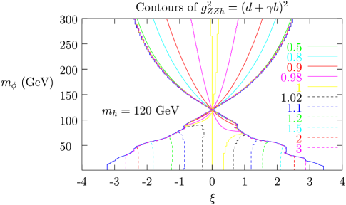
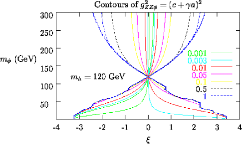
Figure 1: Contours of $g_{ZZh}^{2}=g_{fVh}^{2}$ and $g_{ZZ\phi}^{2}=g_{fV\phi}^{2}$ [defined relative to the SM Higgs, Eq. (4)] for $\Lambda_{\phi}=5~{}{\rm TeV}$ and $m_{h}=120~{}{\rm GeV}$. Regions outside the hour-glass shape are theoretically inconsistent. LEP direct discovery limits have been imposed and (at large $|\xi|$) cut out parts of the otherwise allowed $m_{\phi}<m_{h}$ parameter region. From [?].

The KK-graviton couplings to the $h$ and $\phi$ are determined by $\Lambda_{\phi}$. Fortunately, $\Lambda_{\phi}$ can be extracted using measurements of the KK-graviton spectrum at the LHC. In particular, the mass of the first KK-excitation is given by $m_{1}=x_{1}{m_{0}\over M_{\rm Planck}}{\Lambda_{\phi}\over\sqrt{6}}$, where $x_{1}$ is the first zero of the Bessel function $J_{1}$ ($x_{1}\sim 3.8$), while the excitation spectrum as a function of $m_{jj}$ in the vicinity of $m_{1}$ determines $m_{0}/M_{\rm Planck}$ (see, for example, the plots in [?]). The ratio $m_{0}/M_{\rm Planck}$ is related to the curvature of the brane and should be a relatively small number for consistency of the RS scenario. Sample parameters that are safe from precision EW data and RunI Tevatron constraints are [?] $\Lambda_{\phi}=5~{}{\rm TeV}$ and $m_{0}/M_{\rm Planck}=0.1$ (the latter is employed for all plots presented). These give $m_{1}\sim 780~{}{\rm GeV}$,  well within the LHC reach. Once $\Lambda_{\phi}$ is determined, the goal will be to extract $\xi$, $m_{h}$ and $m_{\phi}$ from Higgs-radion measurements.

Crucial to determining these model parameters are the $f\overline{f}$ and $VV$ couplings of the $h$ and $\phi$. For $V=W,Z$ and all $f$, the $h$ and $\phi$ couplings are rescaled relative to SM $h_{SM}$ couplings by the universal factors $g_{fVh}$ and $g_{fV\phi}$:

$$g_{fVh}=\left(d+\gamma b\right)\,,\quad g_{fV\phi}=\left(c+\gamma a\right)\,.$$ (4)

In contrast, the $gg$ and $\gamma\gamma$ couplings of the $h$ and $\phi$ come from two sources: (1) the standard loop contributions computed using the above $f\overline{f}/VV$ strength factors $g_{fVh}$ or $g_{fV\phi}$; and (2) “anomalous” contributions which are expressed in terms of the SU(3)$\times$SU(2)$\times$U(1) $\beta$ function coefficients. The complicated dependence of $g_{fVh}^{2}$ and $g_{fV\phi}^{2}$ on $\xi$ and $m_{\phi}$ is shown in Fig. 1 for $m_{h}=120~{}{\rm GeV}$ and $\Lambda_{\phi}=5~{}{\rm TeV}$. Note that if $g_{fVh}^{2}<1$ is observed, then $m_{\phi}>m_{h}$, and vice versa, except for a small region near $\xi=0$. Also note that the radion coupling $g_{fV\phi}^{2}$ is generally rather small and exhibits zeroes; however, if $m_{\phi}>m_{h}$ then at large $|\xi|$ the $ZZ\phi$ couplings can become sort of SM strength, implying SM type discovery modes could become relevant (see [?]).

A few notes on branching ratios (see [?]). The $h$ branching ratios are quite SM-like (even if partial widths are different) except that $h\to gg$ can be bigger than normal, especially when $g_{fVh}^{2}$ is suppressed. For $m_{\phi}<2m_{W}$, $\phi\to gg$ is very possibly the dominant mode in the substantial regions near zeroes of $g_{fV\phi}^{2}$. However, for $m_{\phi}>2m_{W}$ the $\phi$ branching ratios are sort of SM-like (except at $\xi\simeq 0$) but total and partial widths are rescaled.

We now turn to the LHC, ILC and $\gamma$C capabilities. We will focus entirely on the case of $m_{h}=120~{}{\rm GeV}$. For the LHC and ILC, we summarize the work of Ref. [?]. For the LHC, we rescaled the statistical significances predicted for the SM Higgs boson at the LHC using $g_{fVh}^{2}$ or $g_{fV\phi}^{2}$ and the modified branching ratios. We found that the most important modes for Higgs-radion discovery are $gg\to h\to\gamma\gamma$ and $gg\to\phi\to ZZ^{(*)}\to 4\ell$. Also useful are $t\overline{t}h$ with $h\to b\overline{b}$ and $gg\to h\to ZZ^{*}\to 4\ell$.

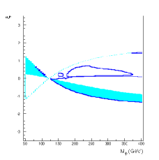
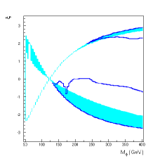
Figure 2: We consider $L=30~{}{\rm fb}^{-1}$ at the LHC for $m_{h}=120~{}{\rm GeV}$. The hour-glass outer boundaries define the theoretically consistent parameter region. Within these, the blank (white) regions are where neither the $gg\to h\to\gamma\gamma$ mode nor the $gg\to h\to 4\ell$ mode yields a $>5\sigma$ signal. The regions between dark blue curves are where $gg\to\phi\to 4\ell$ is $>5\sigma$. The graphs are for $\Lambda_{\phi}=2.5~{}{\rm TeV}$ (left) $\Lambda_{\phi}=5~{}{\rm TeV}$ (center) and $\Lambda_{\phi}=7.5~{}{\rm TeV}$ (right). From [?].

Fig. 2 summarizes our results. It shows that the LHC can find either the $h$ or $\phi$ unless $m_{\phi}<m_{h}$ and $\xi>0~{}\mbox{ and large}$. The region where neither the $h$ nor the $\phi$ can be detected grows (decreases) as $m_{h}$ decreases (increases). It diminishes as $m_{h}$ increases since the $gg\to h\to 4\ell$ rate increases at higher $m_{h}$. The regions where the $h$ is not observable are reduced by considering either a larger data set or $qqh$ Higgs production, in association with forward jets. Figure 2 also exhibits regions at large $|\xi|$ with $m_{\phi}>m_{h}$ in which both the $h$ and $\phi$ mass eigenstates will be detectable. In these regions, the LHC will observe two scalar bosons somewhat separated in mass, with the lighter (heavier) having a non-SM-like rate for the $gg\to h\to\gamma\gamma$ ($gg\to\phi\to ZZ$) final state. Additional information will be required to ascertain whether these two Higgs bosons derive from a multi-doublet or other type of extended Higgs sector or from the present type of model with Higgs-radion mixing. For this, we must turn to the ILC and $\gamma$C.

At an $e^{+}e^{-}$ ILC, any light scalar, $s$, will be detected in the $Z^{*}\to Zs$ mode if $g_{ZZs}^{2}/g_{ZZh_{SM}}^{2}\mathrel{\raise 1.29167pt\hbox{$>$\kern-7.5pt\lower 4.30554pt\hbox{$\sim$}}}0.01$. Since $g_{ZZh}^{2}/g_{ZZh_{SM}}^{2}=g_{fVh}^{2}\geq 0.2$ throughout all of the allowed parameter region, see Fig. 1, observation of the $h$ at the ILC is guaranteed. In contrast, Fig. 1 shows that $g_{fV\phi}^{2}\leq 0.01$ for a significant part of parameter space (smaller $|\xi|$, especially when $m_{\phi}>m_{h}$). Unfortunately, as shown in Ref. [?], this is also the region where precision measurements of the $h$ properties at the ILC will deviate by $\mathrel{\raise 1.29167pt\hbox{$<$\kern-7.5pt\lower 4.30554pt\hbox{$\sim$}}}2.5\sigma$ from SM expectations and we could mistakenly conclude that the Higgs sector was that of the SM.

Can a $\gamma\gamma$ collider at the ILC or $\gamma\gamma$ collider based on a few CLIC modules help? To assess, we recall the results for the SM Higgs boson obtained in the CLIC study of [?]. There, a SM Higgs boson with $m_{h_{SM}}=115~{}{\rm GeV}$ was examined. After cuts, one obtains signal and background rates of $S=3280$ and $B=1660$ in the $\gamma\gamma\to h_{SM}\to b\overline{b}$ channel, corresponding to $S/\sqrt{B}\sim 80$!

First, consider the $h$. By rescaling to obtain $S_{h}$ from $S_{h_{SM}}$, one finds that the $\gamma\gamma\to h\to b\overline{b}$ rate is either changed very little or somewhat enhanced for $m_{\phi}<m_{h}$ and only modestly suppressed for $m_{\phi}>m_{h}$ (e.g. a factor of 2 at $m_{\phi}=200~{}{\rm GeV}$). Thus, at worst, we would have $S_{h}/\sqrt{B}\sim{\textstyle{1\over 2}}80\sim 40$, which is still a very strong signal. In fact, we can afford a reduction by a factor of $16$ before we hit the $5\sigma$ level! Thus, the $\gamma\gamma$ collider will allow $h$ discovery (for $m_{h}=120$) throughout the entire hourglass, which is something the LHC cannot absolutely do. In contrast, using the factor of $16$ mentioned above, the $\phi$ with $m_{\phi}<120~{}{\rm GeV}$ is very likely to elude discovery in the $\gamma\gamma\to\phi\to b\overline{b}$ mode. For the $m_{\phi}>m_{h}$ region, $\gamma\gamma\to\phi\to WW,ZZ$ would be the best mode, but our current results are not encouraging.

It is important to emphasize that the $\gamma$C can play a very special role even if we only observe the $h$ there. Indeed, let us suppose that the $\phi$ is not seen at any of the three colliders. The $h$ is very likely to be seen at the LHC for $L>100~{}{\rm fb}^{-1}$ and, as discussed, will be seen at the $\gamma$C and the ILC. Since $m_{h}$ will be well-measured, only $m_{\phi}$ and $\xi$ need to be determined ($\Lambda_{\phi}$ having been determined as outlined earlier). This requires two measurements, with three or more measurements needed to test the model. If we could trust LHC and $\gamma$C  and ILC absolute rates (systematics being the question), their different dependencies on the parameters imply that we could then determine $m_{\phi}$ and $\xi$ and test the model even if we don’t see the $\phi$. An interesting way to phrase the LHC and $\gamma$C  rate measurements is in terms of the ratio of the rates: ${Rate(gg\to h\to\gamma\gamma)\over Rate(\gamma\gamma\to h\to b\overline{b})}={{\Gamma(gg\to h)\Gamma(h\to\gamma\gamma)\over\Gamma_{h}^{tot}}\over{\Gamma(\gamma\gamma\to h)\Gamma(h\to b\overline{b})\over\Gamma_{h}^{tot}}}={\Gamma(h\to gg)\over\Gamma(h\to b\overline{b})}\,.$ Using this ratio, we may compute

$$R_{hgg}\equiv\left[{\Gamma(h\to gg)\over\Gamma(h\to b\overline{b})}\right]\left[{\Gamma(h_{SM}\to gg)\over\Gamma(h_{SM}\to b\overline{b})}\right]^{-1}\,,$$ (5)

which is the most direct probe for the presence of the anomalous $ggh$ coupling [?]. In particular, $R_{hgg}=1$ if the only contributions to $\Gamma(h\to gg)$ come from quark loops and all quark couplings scale in the same way. Since the RS model predicts anomalous $gg$ coupling contributions in addition to rescaled standard loop contributions, substantial deviations from $R_{hgg}=1$ are predicted, as shown in Fig. 3.

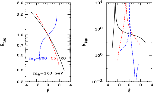
Figure 3: We plot the ratios $R_{hgg}$ and $R_{\phi gg}$ obtained after including the anomalous $ggh$ and $gg\phi$, respectively, coupling contributions. Results are shown for $m_{h}=120~{}{\rm GeV}$ and $\Lambda_{\phi}=5~{}{\rm TeV}$ as functions of $\xi$ for $m_{\phi}=20$, $55$ and $200~{}{\rm GeV}$. (The same type of line is used for a given $m_{\phi}$ in the right-hand figure as is used in the left-hand figure.) From [?].

We can estimate the accuracy with which $R_{hgg}$ can be measured as follows. Assuming the maximal reduction of $S_{h}/S_{h_{SM}}=1/2$, we find that $\Gamma(h\to\gamma\gamma)\Gamma(h\to b\overline{b})/\Gamma_{tot}^{h}$ can be measured with an accuracy of about $\sqrt{S_{h}+B}/S_{h}\sim\sqrt{3200}/1600\sim 0.035$. The dominant error will then be from the LHC which will typically measure $\Gamma(h\to gg)\Gamma(h\to\gamma\gamma)/\Gamma_{tot}^{h}$ with an accuracy of between $0.1$ and $0.2$ (depending on parameter choices and available $L$). From Fig. 3, we see that $0.2$ fractional accuracy will reveal deviations of $R_{hgg}$ from $1$ for all but the smallest $\xi$ values. Given the measured $m_{h}$, the direction and magnitude of those deviations will give a strong constraint on $m_{\phi}$ relative to $\xi$ (although, for instance, you can’t tell if $m_{\phi}<m_{h}$ and $\xi<0$ or $m_{\phi}>m_{h}$ and $\xi>0$).

Now suppose we also observe the $\phi$. If $|\xi|$ is large, this is possible at the ILC for any $m_{\phi}$ (see the $g_{fV\phi}^{2}=0.01$ contour of Fig. 1) and at the LHC if $m_{\phi}>m_{h}$ (see Fig. 2). The value of $R_{hgg}$ combined with knowing $m_{\phi}$ will then determine $\xi$ without relying on any absolute rates. In addition, the $e^{+}e^{-}\to Z^{*}\to Z\phi$ rate will have reliable absolute normalization and it directly determines ${g_{ZZ\phi}^{2}/g_{ZZh_{SM}}^{2}}=g_{fV\phi}^{2}\,.$ Since $g_{fV\phi}^{2}$ is wildly varying as a function of the model parameters (see Fig. 1), its measured value will over constrain and test the model. If the LHC also sees the $\phi$ we get the model-testing $gg\to\phi\to ZZ$ rate, leading to a further cross check on the model.

We summarize assuming that $\Lambda_{\phi}\mathrel{\raise 1.29167pt\hbox{$<$\kern-7.5pt\lower 4.30554pt\hbox{$\sim$}}}20~{}{\rm TeV}$. First, $\Lambda_{\phi}$ will be measured from the KK $m_{jj}$ spectrum at the LHC. Further, for such $\Lambda_{\phi}$, the $\gamma$C, like the ILC, can see a light $h$ for all of the $(\xi,m_{\phi})$ RS parameter space. Both colliders can see the $h$ where the LHC can’t, although the “bad” LHC regions are not very big for full $L$. The ability to measure $R_{hgg}$ may be the strongest reason for having the $\gamma$C as well as the LHC and ILC, not only in the RS context but also since most non-SM Higgs theories predict $R_{hgg}\neq 1$ for one reason or another, unless one is in the decoupling limit. Further, if the $\phi$, as well as the $h$, is detected at the ILC, the motivation for building the $\gamma$C becomes even stronger since the measured values of $m_{h}$, $m_{\phi}$, $R_{hgg}$ and $g_{fV\phi}^{2}$ provide a very definitive over constrained test of the RS model. If $m_{\phi}>m_{h}$ and $|\xi|$ is large enough for detection of $gg\to\phi\to ZZ$ at the LHC to be possible, the ILC would not be critical (but the $\gamma$C would be) since we could get a definitive determination of $\xi$ using the measured $m_{h}$, $m_{\phi}$ and $R_{hgg}$ values and then the $gg\to\phi\to ZZ$ rate would test the model. Further model tests would be possible if we could accurately measure the rate for $h$ production in other LHC and/or $\gamma$C channels — something that is certainly possible, but not guaranteed (especially with high accuracy). Overall, there is a nice complementarity among the machines — each brings new abilities to probe and definitively test the scalar sector of the RS model. Very generally, the case for a (low-energy) $\gamma C$ is compelling if a Higgs boson is seen at the LHC that has non-SM-like rates and properties.

References

References

- [1] L. Randall, R. Sundrum, Phys. Rev. Lett. 83, 3370 (1999) [arXiv:hep-ph/9905221]; Phys. Rev. Lett. 83, 4690 (1999) [arXiv:hep-th/9906064].
- [2] G. Giudice, R. Rattazzi, J. Wells, Nucl. Phys. B595 (2001), 250 [arXiv:hep-ph/0002178].
- [3] C. Csaki, M.L. Graesser, G.D. Kribs, Phys. Rev. D63 (2001), 065002-1 [arXiv:hep-th/0008151].
- [4] D. Dominici, B. Grzadkowski, J. F. Gunion and M. Toharia, Nucl. Phys. B 671, 243 (2003) [arXiv:hep-ph/0206192].
- [5] J. L. Hewett and T. G. Rizzo, JHEP 0308, 028 (2003) [arXiv:hep-ph/0202155]. The results contained in their July 2, 2003 revision of their work are in reasonable agreement with [?].
- [6] J. F. Gunion, M. Toharia and J. D. Wells, Phys. Lett. B 585, 295 (2004) [arXiv:hep-ph/0311219].
- [7] H. Davoudiasl, J. L. Hewett and T. G. Rizzo, Phys. Rev. Lett. 84, 2080 (2000) [arXiv:hep-ph/9909255].
- [8] M. Battaglia, S. De Curtis, A. De Roeck, D. Dominici and J. F. Gunion, Phys. Lett. B 568, 92 (2003) [arXiv:hep-ph/0304245].
- [9] D. Asner et al., Eur. Phys. J. C 28, 27 (2003) [arXiv:hep-ex/0111056].
- [10] D. Asner, el al, arXiv:hep-ph/0208219 and D. Asner et al., arXiv:hep-ph/0308103.