Theory of the endpoint region of exclusive rare B decays

Abstract

In the ratio of ratios of rates for radiative and semileptonic decays of $B$ and $D$ to $K^{*}$ and $\rho$ mesons the non-computable form factors mostly cancel out. The resulting method for the determination of $|V_{ub}|$ is largely free of hadronic uncertainties, raising the prospect of a precise determination of $|V_{ub}|$.

1 Motivation and Results

The third row of the CKM matrix is poorly determined because it involves the top quark. Of the first two rows, the $V_{ub}$ element is the least well known, with a precision of about 20% in its magnitude, $|V_{ub}|$.

The measurement of $|V_{ub}|$ through inclusive charmless semileptonic $B$ decays is complicated by the large background from charm-full semileptonic $B$ decays. Experimentally, cuts may be imposed to suppress or eliminate the background, but this introduces theoretical uncertainties. Some years ago it was guessed[1] that this method would eventually reach a precision of 5%, but by now new complications from theory have been discovered[2], so the eventual precision of the method is expected to be significantly worse.

Alternatively one may look to determine $|V_{ub}|$ from exclusive semileptonic $B$ decays, such as $B\to\pi\ell\nu$ or $B\to\rho\ell\nu$. The difficulty here is from theory: the form factors are not well known. Eventually, unquenched lattice QCD calculations may produce accurate form factors (at least in a restricted region of phase space, but that’s all that is needed to extract $|V_{ub}|$). However, the precision at the moment is no better than[3] 20%.

In this talk I describe a method that relies on exclusive decays which can be used to determine $|V_{ub}|$ to high precision, possibly a couple of percent. The trick is to let experiment, rather than theorists, determine the form factors. Hence, the main result of our work[4, 5, 6]can be framed as a recipe for experiment. Measure the ratio of $B$ decay rates,

$$\frac{{\mbox{d}\Gamma(\bar{B}\to\rho e\nu)}/{\mbox{d}q^{2}}}{{\mbox{d}\Gamma(\bar{B}\to K^{*}\ell^{+}\ell^{-})}/{\mbox{d}q^{2}}}={\frac{|V_{ub}|^{2}}{|V_{tb}V_{ts}^{*}|^{2}}}\cdot\\ \frac{8\pi^{2}}{\alpha^{2}}\cdot\frac{1}{N_{\rm eff}(q^{2})}\frac{\sum_{\lambda}|H_{\lambda}^{B\to\rho}(q^{2})|^{2}}{\sum_{\lambda}|H_{\lambda}^{B\to K^{*}}(q^{2})|^{2}}$$ (1)

Here $q^{2}$ is the invariant mass of the lepton pair and the measurement must be done at large $q^{2}$ (the energy of the $\rho$ or $K^{*}$ in the $B$ rest-frame must not exceed about 500 MeV). The factor $N_{\rm eff}(q^{2})$ is provided by theory. The ratio of helicity amplitudes,

$$R_{B}(y)\equiv\frac{\sum_{\lambda}|H_{\lambda}^{B\to\rho}(y)|^{2}}{\sum_{\lambda}|H_{\lambda}^{B\to K^{*}}(y)|^{2}}$$ (2)

can be obtained experimentally, as follows. Measure decays spectra for $D\to\rho\ell\nu$ and $D\to K^{*}\ell\nu$, and from it construct the ratio

$$R_{D}(y)\equiv\frac{\sum_{\lambda}|H_{\lambda}^{D\to\rho}(y)|^{2}}{\sum_{\lambda}|H_{\lambda}^{D\to K^{*}}(y)|^{2}}$$ (3)

Once the ratios in (2) and (3) are expressed in terms of $y=E_{V}/m_{V}$ ($V=\rho,K^{*}$), one can safely replace one for the other,

$$R_{B}(y)=R_{D}(y)\Big{(}1+{\cal O}(m_{s}(\frac{1}{m_{c}}-\frac{1}{m_{b}}))\Big{)}$$ (4)

In summary, to determine $|V_{ub}|$, measure the ratio of rates in Eq. (1), infer the ratio $R_{B}(y)$ from semileptonic $D$ decays, and combine with the theory-provided $N_{\rm eff}(q^{2})$. At NLL order, $N_{\rm eff}(q^{2}_{\text{max}})=32.76$, varying by 2% as the renormalization scale $\mu$ is varied between 2.4 GeV and 9.6 GeV. The $q^{2}$ dependence is mild (and fully known).

Table 1: Comparison of theoretical predictions of the double-ratio $R_{1}$ of decay constants of heavy mesons

	Method	${f_{B_{s}}}/{f_{B_{d}}}$	${f_{D_{s}}}/{f_{D_{d}}}$	$R_{1}$
	Relativistic Quark Model[8]	1.10$\pm$0.21	1.09$\pm$0.22	1.01$\pm$0.40
	Quenched Lattice[9]	1.16(1)(2)(2)(${}^{+4}_{-0}$)	1.14(1)(${}^{+2}_{-3}$)(3)(1)	1.02(2)(4)(4)(${}^{+4}_{-1}$)
	Unquenched Lattice[10]			1.018$\pm$0.006$\pm$0.010
	Quenched Lattice[11]	1.15$\pm$0.03	1.12$\pm$0.02	1.03$\pm$0.05
	Unquenched Lattice[11]	1.16$\pm$0.05	1.12$\pm$0.04	1.04$\pm$0.08
	QSR[12]	1.16$\pm$0.05	1.15$\pm$0.04	1.01$\pm$0.08
	RSM[13]	1.10$\pm$0.01	1.08$\pm$0.01	1.02$\pm$0.02

2 Theory

2.1 Double ratios

Since the $K^{*}$ and the $\rho$ mesons are similar, one could hope that the hadronic uncertainties would largely cancel in ratios. For example, consider radiative decays:

$$\frac{\Gamma(B\to K^{*}\gamma)}{\Gamma(B\to\rho\gamma)}\propto\left|\frac{F_{B\to K^{*}}(0)}{F_{B\to\rho}(0)}\right|^{2}~{}.$$ (5)

The proportionality factor, which includes calculable phase space, CKM and short distance QCD corrections, has been omitted so that we may focus our attention on the hadronic form factors, $F=F(q^{2})$, which are the main culprits for theoretical uncertainties. In the flavor-$SU(3)$ limit $F_{B\to K^{*}}(0)=F_{B\to\rho}(0)$ so the ratio in (5) is unity. However, flavor-$SU(3)$ symmetry is good to $\sim 30\%$. One may try to improve this situation by guessing that the ratio of form factor is similar to the known ratio of decay constants, $F_{B\to K^{*}}(0)/F_{B\to\rho}(0)\approx f_{K}/f_{\pi}$, but there is no way of assessing precisely the error incurred, so this is not what we want for precision physics.

If we are willing to measure more quantities we can do better. The idea is to construct a ratio of quantities that is fixed to unity by two distinct symmetries. Consider, for example, heavy meson decay constants. In the $SU(3)$ flavor symmetry limit, two ratios are set to unity

$$\frac{f_{B_{s}}}{f_{B}}=1\qquad{\rm and}\qquad\frac{f_{D_{s}}}{f_{D}}=1$$ (6)

Similarly, Heavy Quark Flavor Symmetry fixes different ratios of the same quantities,

$$\frac{f_{B_{s}}}{f_{D_{s}}}=\sqrt{\frac{m_{c}}{m_{b}}}\qquad{\rm and}\qquad\frac{f_{B}}{f_{D}}=\sqrt{\frac{m_{c}}{m_{b}}}$$ (7)

The ratio of ratios can be written as the ratio of the two ratios in either (6) or (7), so it is protected from deviating from 1 by the two symmetries:[7]

$$R_{1}=\frac{f_{B_{s}}/f_{B}}{f_{D_{s}}/f_{D}}=1+{\cal O}\left(m_{s}\left(\frac{1}{m_{c}}-\frac{1}{m_{b}}\right)\right)$$

Table 1 demonstrates how well this works. The ratio $R_{1}$ is computed by different theoretical methods, so the individual decay constants and ratios differ significantly between methods. But because all methods incorporate flavor and heavy quark symmetry the double ratio deviates from unity by a couple of percent in all cases. Similarly estimates of double ratios of form factors in semileptonic decays, $B\to D^{(*)}\ell\nu$[14], $B\to(K^{*},\rho)\ell\nu$[15] and $B\to(K,\pi)\ell\nu$[16], give deviations from unity of a few percent.

2.2 Double ratio in $B\to\rho\ell\nu$

Ligeti and Wise[17] studied the use of double ratios in the determination of form factors in $B\to\rho\ell\nu$. By measuring form factors in $B\to K^{*}\ell^{+}\ell^{-}$, $D\to K^{*}\ell\nu$ and $D\to\rho\ell\nu$ one can use a double ratio to determine

$$f^{(B\to\rho)}\approx f^{(B\to K^{*})}\,\frac{f^{(D\to\rho)}}{f^{(D\to K^{*})}}~{}.$$ (8)

There are three stumbling blocks to complete this program:[4]

1. The rates depend on several form factors, but the double ratio relates individual form factors. Measuring individual form factors places additional demands on experimental measurements.

2. There are form factors in $B\to K^{*}\ell^{+}\ell^{-}$ that are not present in the semileptonic decays.

3. There are long distance contributions to $B\to K^{*}\ell^{+}\ell^{-}$ (mostly from $B\to K^{*}(c\bar{c})$ with $(c\bar{c})\to\ell^{+}\ell^{-}$).

We address each problem in turn.

Figure 1: Example of non-factorizable diagram contributing to the “long-distance” amplitude for $B\to K^{*}\ell^{+}\ell^{-}$

The solution to problem #1 above is trivial. Let’s ignore for now the additional form factors from tensor operators that enter $B\to K^{*}\ell\ell$ (difficulty #2, above). Consider the semileptonic decay rate

$$\frac{d\Gamma(\bar{B}\to\rho e\nu)}{dq^{2}}=\frac{G_{F}^{2}|V_{ub}|^{2}}{96\pi^{3}m_{B}^{2}}q^{2}|\vec{q}|\!\!\!\sum_{\lambda=\pm,0}\!\!\!|H_{\lambda}|^{2}$$ (9)

Here $H_{\lambda}$, $\lambda=\pm,0$ are helicity amplitudes. The point is that the double ratio technique can be applied directly to the sums $\sum_{\lambda=\pm,0}|H_{\lambda}|^{2}$. If we were comparing $(B\to\rho\ell\nu)/(B\to K^{*}\ell\nu)$ to $(D\to\rho\ell\nu)/(D\to K^{*}\ell\nu)$ we would have accomplished our goal. The problem is that there is no $B\to K^{*}\ell\nu$ decay. So we consider $B\to K^{*}\ell\ell$ instead, but this introduces the additional complications #2 and #3.

To address these issues, recall that the effective $\Delta B=-\Delta S=1$ Hamiltonian,

$${\cal H}_{\rm eff}=-\frac{G_{F}}{\sqrt{2}}V_{tb}V_{ts}^{*}\sum_{i=1}^{10}C_{i}(\mu)Q_{i}(\mu)\,,$$

has four-quark operators $Q_{1}$–$Q_{6}$, e.g., $Q_{2}=(\bar{s}c)_{V-A}(\bar{c}b)_{V-A}$, a transition magnetic moment operator,

$$Q_{7}=\frac{e}{8\pi^{2}}m_{b}\bar{s}_{\alpha}\sigma_{\mu\nu}(1+\gamma_{5})b_{\alpha}F_{\mu\nu},$$ (10)

an analogous color moment operator $Q_{8}$, and vector and axial current operators

$$Q_{9,10}=\frac{e^{2}}{8\pi^{2}}(\bar{s}b)_{V-A}(\bar{e}e)_{V,A}$$ (11)

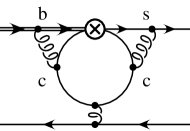
The Wilson coefficients $C_{9,10}$ are larger than the rest. Roughly, at $\mu=m_{b}$ one has $C_{9,10}\approx 5$, $C_{2}\approx 1$, $C_{1,7}\approx 1/3$, and the rest much smaller. This is good news, since the matrix elements of $Q_{9,10}$ are given in terms of the same form factors as for the semileptonic decay.

The rate for $B\to K^{*}\ell\ell$ depends on the tensor form factors from the operator $Q_{7}$. These form factors are given in terms of the vector and axial form factors of the semileptonic decays up to $1/m_{Q}$ corrections by heavy quark symmetry, provided $y\sim 1$ (recall $y=E_{V}/m_{V}$). One may write the rate in terms of helicity amplitudes

$$\frac{d\Gamma(B\to K^{*}e^{+}e^{-})}{dq^{2}}=\frac{4G_{F}^{2}|V_{tb}V_{ts}^{*}|^{2}\alpha^{2}}{3m_{B}^{2}(4\pi)^{5}}\times\\ q^{2}|\vec{q}\,|\sum_{\lambda=\pm 1,0}\left\{|H_{\lambda}^{(V)}|^{2}+|H_{\lambda}^{(A)}|^{2}\right\}\,,$$ (12)

and the form factor relations give

$$H_{\lambda}^{(V)}(q^{2})=C_{9}\Big{(}1+\delta(q^{2})+{{\cal O}}(\Lambda/m_{b})\Big{)}H_{\lambda}(q^{2}),$$ (13)

where $\delta(q^{2})=({2m_{b}^{2}}/{q^{2}})({C_{7}}/{C_{9}})$. It is not the smallness of the correction $\delta(q^{2})$ that matters, since it is computable. Rather, it is that the corrections to the form factor relations, denoted by “${{\cal O}}(\Lambda/m_{b})$”, have an additional suppression of $C_{7}/C_{9}\sim 10^{-1}$ allowing for high precision in the method.

Finally we have to deal with the contributions of the operators $Q_{1}$–$Q_{6}$. These are the long-distance effects of difficulty #3 listed above. Note, however, that the use of form factor relations has forced us to work at $q^{2}$ near $q^{2}_{\text{max}}=(M_{B}-M_{K^{*}})^{2}$. This is well above the threshold for charm pair production. Since $q^{2}$ is large we can perform an operator product expansion (OPE) in inverse powers of $q^{2}$. To avoid positive powers of $m_{b}^{2}$ it is best to take $\sqrt{q^{2}}\sim m_{b}$ and expand in both large scales simultaneously. The “long-distance effect” is replaced by a sum of local terms that can be truncated given a desired accuracy.

Figure 2: ALEPH’s[18] charged current form factor from $\tau$ decay. Local quark-hadron duality is a poor approximation in the resonant region but quickly improves a few GeV² above that.

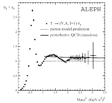
The good news is that the leading terms in the expansion give rise to computable amplitudes: they are expressed in terms of the same form factors that appear in semileptonic decays. The bad news is that this OPE is performed in the time-like region. It is applicable only to the extent that quark-hadron duality is a good approximation. Fig. 2 shows how quark hadron duality works in one example, the form factor for the charged current obtained from $\tau$ decay data. The bad news is not so bad: since the “long-distance” effect is a small contribution to the $B\to K^{*}\ell\ell$ rate, one can tolerate a 50% error in quark-hadron duality without spoiling the determination of $|V_{ub}|$ to a few percent accuracy. Notice also that no assumption of factorization was made.

References

- [1] C. W. Bauer, Z. Ligeti and M. E. Luke, Phys. Rev. D 64, 113004 (2001); and Phys. Lett. B 479, 395 (2000)
- [2] M. B. Voloshin, Phys. Lett. B 515, 74 (2001); and Mod. Phys. Lett. A 17, 245 (2002); K. S. M. Lee and I. W. Stewart, arXiv:hep-ph/0409045.
- [3] S. Hashimoto, these proceedings.
- [4] B. Grinstein and D. Pirjol, arXiv:hep-ph/0404250.
- [5] B. Grinstein and D. Pirjol, Phys. Lett. B 549, 314 (2002)
- [6] B. Grinstein and D. Pirjol, Phys. Lett. B 533, 8 (2002)
- [7] B. Grinstein, Phys. Rev. Lett. 71, 3067 (1993)
- [8] D. Ebert, R. N. Faustov and V. O. Galkin, Mod. Phys. Letts. A17 (2002) 803.
- [9] C. Bernard et al., Phys. Rev. D66 (2002)094501.
- [10] T.Onogi et al., Nucl. Phys. Proc. Suppl. 119 (2003) 610.
- [11] S. Ryan, Nucl. Phys. Pro. Suppl. 106 (2002) 86.
- [12] S. Narison, Phys. Letts. B520 (2001) 115.
- [13] G. Cvetic et al, Phys. Lett. B 596, 84 (2004)
- [14] C. G. Boyd and B. Grinstein, Nucl. Phys. B 451, 177 (1995)
- [15] Z. Ligeti, I. W. Stewart and M. B. Wise, Phys. Lett. B 420, 359 (1998)
- [16] C. G. Boyd and B. Grinstein, Nucl. Phys. B 442, 205 (1995)
- [17] Z. Ligeti and M. B. Wise, Phys. Rev. D 53, 4937 (1996)
- [18] R. Barate et al. [ALEPH Collaboration], Eur. Phys. J. C 4, 409 (1998).