Determining $\alpha$ and $\gamma$ - theory

In this short review presented at FPCP04, Daegu, Korea, we discuss methods leading to determinations of $\alpha$ and $\gamma$ with practically no theoretical error. The remaining theoretical errors due to isospin breaking, neglecting of electroweak penguins or coming from other sources are addressed.

1 Introduction

We are entering a period of time, when direct determinations of the angles $\alpha$ and $\gamma$ of the standard unitarity triangle are becoming possible. In this talk we will review the methods that are used at present and the related theoretical uncertainties. Surprisingly enough, some of the most useful methods were not even talked about before 2003. The questions that will be addressed are therefore (i) what is the ultimate precision of different methods and (ii) what are we learning about $\alpha,\gamma$ now? The last question has been covered in great detail in talks by experimental colleagues [1], so only the final results will be given here.

How can one measure $\alpha$ and $\gamma$? The sensitivity to the phases comes from interference. Useful methods thus rely on channels with at least two interfering amplitudes and/or interference between mixing and decay. In order to extract the weak phases, however, one needs to evaluate unknown hadronic parameters that also enter the obsevables. A conservative approach to this problem is to extract all the hadronic parameters from experiment. This is accomplished by using symmetries of QCD (e.g. $C$, $P$, isospin), and by finding channels, where all parameters are obtainable from experiment. Another approach is to calculate the hadronic parameters using theoretical frameworks like QCD factorization, PQCD, and SCET. This later avenue will not be exploited here and the reader is referred to [2] for further details.

2 Measuring $\alpha$

2.1 $B(t)\rightarrow\pi\pi$

This method is due to Gronau and London and dates back almost 15 years ago [3]. Let us review the method step by step to see where the approximations enter. A completely general isospin decomposition of the decay amplitudes is

$$\begin{split}A_{+-}&=\langle\pi^{+}\pi^{-}|H|B^{0}\rangle=-A_{1/2}+\tfrac{1}{\sqrt{2}}A_{3/2}-\tfrac{1}{\sqrt{2}}A_{5/2},\\ A_{00}&=\langle\pi^{0}\pi^{0}|H|B^{0}\rangle~{}=\tfrac{1}{\sqrt{2}}A_{1/2}+A_{3/2}\qquad-A_{5/2},\\ A_{+0}&=\langle\pi^{+}\pi^{0}|H|B^{+}\rangle=\qquad\qquad\tfrac{3}{2}A_{3/2}\quad+A_{5/2},\end{split}$$ (1)

where the notation for the reduced matrix elements is $A_{\Delta I}$. Equivalent relations hold for $\overline{B}^{0}$, $B^{-}$ decay amplitudes $\overline{A}_{+-}$, $\overline{A}_{00}$, $\overline{A}_{+0}$. Note that the $\Delta I=5/2$ operators are not present in the effective weak Lagrangian, so that $A_{5/2}$ can only arise from isospin breaking final state rescattering effects, such as $\Delta I=2$ electromagnetic rescattering of two pions. One can thus estimate $A_{5/2}\sim\alpha A_{1/2}$. Setting $A_{5/2}=0$ therefore means neglecting a $\sim 1\%$ correction. Making this approximation one obtains two triangle relations

$$A_{+-}+\sqrt{2}\;A_{00}=\sqrt{2}\;A_{+0},\qquad\qquad\overline{A}_{+-}+\sqrt{2}\;\overline{A}_{00}=\sqrt{2}\;\overline{A}_{+0}.$$ (2)

Aside from possible electroweak penguin operator (EWP) contributions, $A_{+0}$ is a pure tree. Neglecting EWP one has an additional relation

$$e^{i\gamma}A_{+0}=e^{-i\gamma}\overline{A}_{+0}\quad~{}\Rightarrow~{}\quad|A_{+0}|=|\overline{A}_{+0}|.$$ (3)

This allows to extract $\sin 2\alpha$ from $\Gamma(B^{0}(t)\rightarrow\pi^{+}\pi^{-})\propto[1+C_{\pi\pi}\cos\Delta mt-S_{\pi\pi}\sin\Delta mt]$ using the construction of Gronau and London [3]. The observable $\sin(2\alpha_{\rm eff})=S_{\pi\pi}/\sqrt{1-C_{\pi\pi}^{2}}$ is directly related to $\alpha$ through $2\alpha=2\alpha_{\rm eff}-2\theta$, where $\theta$ is defined on Fig. 1.

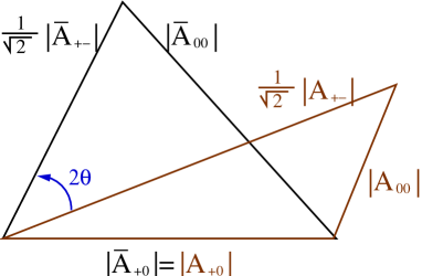
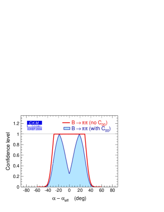
Figure 1: Left: presentation of Eqs. (2), (3), due to Gronau and London [3]. Only one of four possible triangle orientations is shown. Right: constraints on $\alpha-\alpha_{\rm eff}$ from isospin analysis [5].

The difficulty of this approach is the need to distinguish between $B^{0}\rightarrow\pi^{0}\pi^{0}$ and $\overline{B}^{0}\rightarrow\pi^{0}\pi^{0}$ decays, i.e. the need to measure the sides $A_{00}$ and $\overline{A}_{00}$ of the triangle relations (see Fig. 1). Since the summer of 2004 at least a preliminary isospin analysis is possible, as first measurements of $B^{0}(\overline{B}^{0})\rightarrow\pi^{0}\pi^{0}$ rates became available, $C_{00}=-0.28\pm 0.39$ and $Br(B\rightarrow\pi^{0}\pi^{0})=(1.51\pm 0.28)\cdot 10^{-6}$ [4]. Taking a simple weighted average of Belle and BaBar results on $B(t)\rightarrow\pi^{+}\pi^{-}$ (see Table 1), the isospin analysis would at present lead to the constraint on $\alpha-\alpha_{\rm eff}$ shown on Fig. 1 [5]. One does see two emerging peaks when information on $A_{00},\overline{A}_{00}$ is included, however more data is needed to constrain $\alpha-\alpha_{\rm eff}$. At present

$$|\alpha-\alpha_{\rm eff}|<39^{\circ}\qquad(90\%{\rm~{}CL}).$$ (4)

Furthermore the interpretation of $\alpha$ is far from clear due to marginal consistency of $S_{\pi\pi}$ measurements, Table 1. Recently it was also noted that $\alpha_{\rm eff}>\alpha$, if the magnitude and phase of penguin contributions is not too large [6].

$B\rightarrow\pi^{+}\pi^{-}$	$\sin 2\alpha_{\rm eff}$	$C_{\pi^{+}\pi^{-}}$
BABAR [8]	$-0.30\pm 0.17$	$-0.09\pm 0.15$
BELLE [9]	$-1.00\pm 0.22$	$-0.58\pm 0.17$
average	$-0.61\pm 0.14$	$-0.37\pm 0.11$

Table 1: Experimental values of observables in $B\rightarrow\pi^{+}\pi^{-}$.

Let us now return to the question of theoretical uncertainties in the isospin analysis [7]. There are two sources of isospin breaking: (i) $d$ and $u$ charges are different, and (ii) $m_{u}$ does not equal $m_{d}$. The difference of the light quark charges results in additional operators, the electroweak penguin operators, in the effective weak hamiltonian. Including EWP in the analysis will not affect the separate triangle relations (2), but only the additional relation (3), since $A_{0+}$ no longer receives only tree contributions. Remarkably enough, there exist a relation [10, 11]

$$H_{\rm eff,~{}EWP}^{\Delta I=3/2}=-\frac{3}{2}\frac{C_{9}+C_{10}}{C_{1}+C_{2}}\left|\frac{V_{tb}^{*}V_{td}}{V_{ub}^{*}V_{ud}}\right|H_{\rm eff,~{}c-c}^{\Delta I=3/2}$$ (5)

which makes the inclusion of EWP fairly straightforward. Instead of Eq. (3) one has

$$e^{i\gamma}A_{+0}=e^{-i(\gamma+{\delta})}\overline{A}_{+0},$$ (6)

where $\delta\sim 1.5^{\circ}$ [11]. The only assumption that entered this estimate is the dominance of EWP operators $Q_{9,10}$, while no estimate of matrix elements is needed. Note that still $|A_{+0}|=|\overline{A}_{+0}|$. Deviations from this relations would therefore not test the presence of EWP but only the size of the Wilson coefficient suppressed EWP operators $Q_{7,8}$. Note as well, that the same relation $e^{i\gamma}T=e^{-i(\gamma+{\delta})}\overline{T}$ holds also for $\Delta I=3/2$ (tree) amplitudes in the $\rho\rho$ and $\rho\pi$ systems.

Nonzero $m_{u}-m_{d}$ difference results in $\pi^{0}-\eta-\eta^{\prime}$ mixing, i.e. $\pi^{0}$ wave function has small $\eta,\eta^{\prime}$ admixtures. Because of this Gronau-London triangle relations (2) no longer hold [12]. Gardner [12] found that this typically leads to $\Delta\alpha\sim 5^{\circ}$ shift in the extracted value of $\alpha$. Since we now have more experimental data about the $\pi\pi$ system it would be interesting to reevaluate this effect, especially if the analysis is extended beyond factorization that was used in [12]. The analysis of [12] also showed that $\Delta\alpha$ depends on the value of $P/T$ and will thus be different for $\rho\rho$, $\rho\pi$ systems, where no such quantitative analysis exists at present.

2.2 Measurement of $\alpha$ from $B\rightarrow\rho\rho$

The isospin analysis in $B\rightarrow\rho\rho$ follows the same lines as for $B\rightarrow\pi\pi$, but with three separate isospin relations (2), one for each polarization. However, longitudinally polarized final state dominates the other two, $f_{L}^{+-}=0.99\pm 0.03^{+0.04}_{-0.03}$ [13] and $f_{L}^{+0}=0.97^{+0.03}_{-0.07}\pm 0.04$ [14]. This simplifies the analysis as there is effectively only one isospin relation. Another difference from the $\pi\pi$ system is that $\rho$ resonances have a nonnegligible decay width. The invariant mass measured from the decay products can thus differ from the pole mass of the $\rho$ resonance. The two $\rho$ resonances in the final state can therefore also form an $I=1$ state, if the respective invariant masses are different [15]. This affects the analysis at $O(\Gamma_{\rho}^{2}/m_{\rho}^{2})$. As shown in [15] it is possible to constrain this effect experimentally by making different fits to the mass distributions.

An ingredient that makes the $\rho\rho$ system favorable over $\pi\pi$ is a small penguin pollution, as can be inferred from the bound $Br(B\rightarrow\rho^{0}\rho^{0})<1.1\cdot 10^{-6}(90\%{\rm~{}CL})$ [16] (cf. also Fig. 1). This gives a measurement of $\alpha$ from $S_{\rho^{+}\rho^{-}}$ using isospin analysis [16]

$$\alpha=[96\pm 10\pm 4\pm{11}]^{\circ},$$ (7)

with the last error representing the ambiguity due to the presence of penguins. In obtaining the above result isospin breaking effects, EWP, non-resonant and $I=1$ contributions were neglected.

2.3 $B\rightarrow\rho\pi$

Since $\rho^{\pm}\pi^{\mp}$ are not CP eigenstates, extracting $\alpha$ from this system is more complicated. There are essentially two approaches, (i) either one uses the full $B(t)\rightarrow\pi^{+}\pi^{-}\pi^{0}$ Dalitz plot together with isospin [17], or (ii) one uses only the $\rho^{\pm}\pi^{\mp}$ region together with SU(3) related modes [18].

If the full $B\rightarrow\pi^{+}\pi^{-}\pi^{0}$ Dalitz plot is used, one needs to model the Dalitz plot, for instance as a fit to a sum of Breit-Wigner forms

$$f(B^{0}\rightarrow 3\pi)=BW(s_{+})\underbrace{A(B^{0}\rightarrow\rho^{+}\pi^{-})}_{A_{+}}+BW(s_{-})\underbrace{A(B^{0}\rightarrow\rho^{-}\pi^{+})}_{A_{-}}+BW(s_{0})\underbrace{A(B^{0}\rightarrow\rho^{0}\pi^{0})}_{A_{0}},$$ (8)

where for simplicity only $\rho$ resonances were kept in the sum, but other resonance can be added. From time dependent $B(t)\rightarrow 3\pi$ Dalitz plot analysis one has 27 real observables, of which 18 measure the interference between different $\rho$ resonance bands. In this way it is possible to determine $A_{\pm,\;0}$, $\overline{A}_{\pm,\;0}$, up to an overall phase, i.e. there are 11 independent measurables. A potential problem can arise from the fact that the peaks of $\rho$ resonance bands do not overlap, but are separated by approximately one decay width. To measure the 11 observables correctly one therefore has to model the tails of the resonances correctly.

In order to extract $\alpha$ from $A_{\pm,\;0}$, $\overline{A}_{\pm,\;0}$ additional input is needed. First let us define tree and penguin contributions according to whether or not they contain CKM weak phase

$$A_{\pm}=e^{i\gamma}t_{\pm}+p_{\pm},\qquad\qquad A_{0}=e^{i\gamma}t_{0}+p_{0},$$ (9)

and similarly for $\overline{A}_{\pm},\overline{A}_{0}$, but with a sign of $\gamma$ flipped. The $\Delta I=3/2$ part of the weak hamiltonian has a CKM phase, so the penguins $p_{\pm,0}$ are purely $\Delta I=1/2$ (neglecting EWP). This leads to an isospin relation [17, 19]

$$p_{0}=-\tfrac{1}{2}(p_{+}+p_{-}),$$ (10)

which reduces the number of unknowns to 10. One possible choice of unknowns is $\alpha$, $|t_{\pm}|$, $|t_{0}|$ $\arg t_{\pm}$, $|p_{\pm}|$, $\arg p_{\pm}$. There is thus enough information to determine all of them. Explicitly, the observable that gives $\alpha$ directly is

$$A_{+-}+A_{-+}+2A_{00}=T\Rightarrow-\operatorname{Im}\left(\tfrac{q}{p}\tfrac{\overline{T}}{T}\right)=\sin(2\alpha).$$ (11)

There are some further comments that apply to the Snyder-Quinn method. As already stated, the effects due to isospin breaking have not been analysed quantitatively yet. However, isospin breaking will enter only in relation (10). Since penguins are small, $|p_{\pm}/t_{\pm}|\sim 20\%$ [18], it is reasonable to expect that isospin breaking effects will also be small, or at least smaller than in the $B\rightarrow\pi\pi$ case. In addition, if $A_{5/2}\neq 0$, only the part of $A_{5/2}$ that has the same weak phase as $p_{\pm,0}$ will affect the analysis by modifying the relation in Eq. (10). These contributions would come from electromagnetic final state rescatering of penguin contributions, leading to negligible effect.

BaBar performed the Snyder-Quinn analysis (but keeping 10 out of 27 observables fixed to zero), obtaining [20]

$$\alpha=(113^{+27}_{-17}\pm 6)^{\circ}.$$ (12)

Note that there is only one solution in $[0^{\circ},180^{\circ})$.

The potential problem of having to model the tails of the $\rho$ bands can be avoided by using just the $\rho^{\pm}\pi^{\mp}$ final state and the $SU(3)$ related modes [18]. As in (9), the tree and penguin contributions are defined according to their weak phases. In total there are 8 unknowns: $|t_{\pm}|$, $|p_{\pm}|$, $\arg\big{(}p_{\pm}/t_{\pm}\big{)}$, $\arg\big{(}t_{-}/t_{+}\big{)}$, $\alpha$, but just 6 observables. Additional infromation on penguin contributions can be obtained from SU(3) related $\Delta S=1$ modes, in which penguins are CKM enhanced and tree terms CKM suppressed compared to the $\rho^{\pm}\pi^{\mp}$ final state. Since penguin contributions are small, the error introduced because of the SU(3) breaking will not be large. Note that in order to relate the $\Delta S=1$ and $\Delta S=0$ channels, annihilation like topologies were neglected.

To resolve ambiguties an additional assumption of $\arg(t_{-}/t_{+})$ being smaller than $90^{\circ}$ had to be used. This leads to

$$\alpha=(94\pm 4\pm{15})^{\circ}$$ (13)

with the last error the combined error coming from $\alpha-\alpha_{\rm eff}$ difference and the estimate of SU(3) breaking effects. To obtain this number no interference information was used (i.e. experimental data from both BaBar [20] and Belle [21] was used). Also, only bounds on penguins were used, not a complete SU(3) fit. In the future an unconstrained fit to obtain $\alpha$ could be performed. This would lead to a single solution for $\alpha$, with all ambiguities resolved. As already stated, the SU(3) breaking on extracted $\alpha$ would be small, of order $p_{\pm}^{2}/t_{\pm}^{2}$. A Monte Carlo study with up to $30\%$ SU(3) breaking on penguins for instance gives $\sqrt{\langle(\alpha^{\rm out}-\alpha^{\rm in})^{2}\rangle}\sim 2^{\circ}$ [18].

3 Measuring $\gamma$

3.1 $B^{\pm}\rightarrow DK^{\pm}$

There are many methods that fall into this class, all of which use the interference between $b\rightarrow c\overline{u}s$ and $b\rightarrow u\overline{c}s$ [22]. In the case of charged $B$ decays this means that the interference is between $B^{-}\rightarrow DK^{-}$ followed by $D\rightarrow f$ decay and $B^{-}\rightarrow\overline{D}K^{-}$ followed by $\overline{D}\rightarrow f$, where $f$ is any common final state of $D$ and $\overline{D}$. What makes this method very powerful is that there are no penguin contributions and therefore almost no theoretical uncertainties, with all the hadronic unknowns in principle obtainable from experiment (with problems in measuring color suppressed $B^{-}\rightarrow\overline{D^{0}}K^{-}$ decay [23]).

Different methods can be grouped according to the choice of the final state $f$, which can be (i) a CP- eigenstate (e.g. $K_{S}\pi^{0}$) [22], (ii) a flavor state (e.g. $K^{+}\pi^{-}$) [23] , (iii) a singly Cabibbo suppressed (e.g. $K^{*+}K^{-}$) [24] or (iv) a many-body final state (e.g. $K_{S}\pi^{+}\pi^{-}$) [25]. There are also other extensions: many body $B$ final states (e.g. $B^{+}\rightarrow DK^{+}\pi^{0}$) [26], $D^{0*}$ in addition to $D^{0}$, self tagging $D^{0**}$ [27] or neutral $B$ decays (time dependent and time-integrated) can be used [29, 28].

In this talk we focus on extracting $\gamma$ from $B^{\pm}\rightarrow(K_{S}\pi^{+}\pi^{-})_{D}K^{\pm}$, since this is experimentally most advanced. Both experiments use $D^{*}$ and $D$ decays, where a subtelty of a sign flip in the use of $D^{*}$ has been pointed out only recently [30]. The BaBar result [31]

$$\gamma=(88\pm 41\pm 19\pm 10)^{\circ},$$ (14)

should therefore be treated as preliminary only. Belle on the other hand obtains [32]

$$\gamma=(68^{+14}_{-15}\pm 13\pm 11)^{\circ}.$$ (15)

Note that only a single solution for $\gamma$ is obtained in $[0,180)^{\circ}$ range.

For details on how the method works see [25, 31, 32, 33]. We will just make several statements regarding the remaining theoretical errors. First of all, it is possible to extend this approach beyond Breit-Wigner fits of Dalitz plot, so that there is no modeling error left [25, 34]. Also, the effect of $D-\overline{D}$ mixing is included automaticaly, if $D^{*}$ tagged $D$ decays are used to measure the observables of $D$ system. The largest remaining theoretical error is due to possible direct CP violation in the $D$ decay, which is, however, highly CKM suppressed by $\lambda^{5}\sim 5\cdot 10^{-4}$. The measurement of $\gamma$ will therefore be dominated by experimental errors for years to come.

3.2 $\gamma$ from $B(t)\rightarrow D^{(*)+}D^{(*)-}$

This is a very recent method [35]. Again, the amplitude is split into tree and penguin according to CKM

$$A_{D}=A(B^{0}\rightarrow D^{+}D^{-})=\underbrace{t}_{V_{cb}^{*}V_{cd}}+\underbrace{pe^{i\gamma}}_{V_{ub}^{*}V_{ud}}$$ (16)

Value of $t$ is determined from $B^{0}\rightarrow D_{s}^{+}D^{-}$ using SU(3) with leading SU(3) breaking correction accounted for $\frac{t^{\prime}}{t}=\frac{V_{cs}}{V_{cd}}\frac{f_{D_{s}}}{f_{D}}$, with subleading corrections estimated to be below $5\%-10\%$. At present additional approximations are needed to obtain bounds on $\gamma$ from $D^{*+}D^{-}$, $D^{*+}D^{*-}$. This leads to three viable regions for $\gamma$ at $68\%$ CL, $\gamma\in[19.4^{\circ},80.6^{\circ}]$ or $\gamma\in[120^{\circ},147^{\circ}]$ or $\gamma\in[160^{\circ},174^{\circ}]$.

3.3 $\sin(2\beta+\gamma)$

The combination $\sin(2\beta+\gamma)$ can (at least in principle) be extracted very cleanly from the time dependent measurement $B(t)\rightarrow D^{(*)}\pi^{-}$ [36]. Until the small direct CP asymmetry is measured, however, the weak phase $\gamma$ and the strong phase $\delta$ can be extracted from $S_{D^{(*)\pm}\pi^{\mp}}={2r}/({1+r^{2}})\cdot\sin(2\beta+\gamma\pm\delta)$ only, if the ratio of the two interfering amplitudes $r=|A(B^{0}\rightarrow D^{(*)+}\pi^{-})/A(\overline{B}^{0}\rightarrow D^{(*)+}\pi^{-})|$ is known. This ratio can be obtained using $SU(3)$ from $Br(B^{0}\rightarrow D_{s}^{(*)+}\pi^{-})$. Assuming factorization, taking $f_{D_{s}^{(*)}}/f_{D^{(*)}}$ from lattice, and neglecting (very) small anihhilation like diagrams, this gives $r_{D\pi}=0.019\pm 0.04$, $r_{D^{*}\pi}=0.017^{+0.005}_{-0.007}$. Using this number BaBar obtains $|\sin(2\beta+\gamma)|>0.58~{}(90\%{\rm~{}CL})$ from partially reconstructed $B\rightarrow D^{*\mp}\pi^{\pm}$ [37].

4 Conclusions

In conclusion, we have working tools to determine angles $\alpha$ and $\gamma$ of the CKM unitarity triangle. The experimental situation looks much more favorable than expected a few years ago. For instance, measurements of $\alpha$ are already reaching precision level, where one has to start worrying about theoretical errors.
Acknowledgements
I thank Y. Grossman and M. Gronau for carefully reading the manuscript.

References

- [1] See talks by J. Albert, A. Bevan, T. Gershon, and D. Lange, these proceedings.
- [2] See talks by Hai-Yang Cheng, Yong-Yeon Keum, D. Pirjol, these proceedings.
- [3] M. Gronau and D. London, Phys. Rev. Lett. 65, 3381 (1990).
- [4] K. Abe et al. [Belle Collaboration], hep-ex/0408101; B. Aubert et al. [BABAR Collaboration], hep-ex/0408081.
- [5] This figure was made by A. Hoecker and presented by Z. Ligeti at International Conference on High-Energy Physics, ICHEP 04, Beijing, China, hep-ph/0408267.
- [6] M. Gronau, E. Lunghi and D. Wyler, hep-ph/0410170.
- [7] See also M. Ciuchini, talk at CKM angles and BaBar planning workshop, SLAC, 2003, http://www.slac.stanford.edu/BFROOT/www/Public/Physics/ckm2003_workshop/ciuchini.pdf
- [8] B. Aubert et al. [BABAR Collaboration], hep-ex/0408089.
- [9] K. Abe et al. [Belle Collaboration], Phys. Rev. Lett. 93, 021601 (2004).
- [10] M. Neubert and J. L. Rosner, Phys. Lett. B 441, 403 (1998); A. J. Buras and R. Fleischer, Eur. Phys. J. C 11, 93 (1999).
- [11] M. Gronau, D. Pirjol and T. M. Yan, Phys. Rev. D 60, 034021 (1999) [Erratum-ibid. D 69, 119901 (2004)].
- [12] S. Gardner, Phys. Rev. D 59, 077502 (1999).
- [13] B. Aubert et al. [BABAR Collaboration], hep-ex/0404029.
- [14] B. Aubert et al. [BABAR Collaboration], Phys. Rev. Lett. 91, 171802 (2003).
- [15] A. F. Falk, Z. Ligeti, Y. Nir and H. Quinn, Phys. Rev. D 69, 011502 (2004).
- [16] C. Dallapiccola, talk at ICHEP 04, [5].
- [17] A. E. Snyder and H. R. Quinn, Phys. Rev. D 48, 2139 (1993).
- [18] M. Gronau and J. Zupan, hep-ph/0407002.
- [19] H. J. Lipkin, Y. Nir, H. R. Quinn and A. Snyder, Phys. Rev. D 44, 1454 (1991).
- [20] B. Aubert et al. [BABAR Collaboration], hep-ex/0408099.
- [21] C. C. Wang et al. [Belle Collaboration], hep-ex/0408003.
- [22] M. Gronau and D. Wyler, Phys. Lett. B 265, 172 (1991); M. Gronau and D. London., Phys. Lett. B 253, 483 (1991).
- [23] D. Atwood, I. Dunietz and A. Soni, Phys. Rev. Lett. 78, 3257 (1997); D. Atwood, I. Dunietz and A. Soni, Phys. Rev. D 63, 036005 (2001).
- [24] Y. Grossman, Z. Ligeti and A. Soffer, Phys. Rev. D 67, 071301 (2003).
- [25] A. Giri, Y. Grossman, A. Soffer and J. Zupan, Phys. Rev. D 68, 054018 (2003).
- [26] R. Aleksan, T. C. Petersen and A. Soffer, Phys. Rev. D 67, 096002 (2003). M. Gronau, Phys. Lett. B 557, 198 (2003).
- [27] N. Sinha, hep-ph/0405061.
- [28] B. Kayser and D. London, Phys. Rev. D 61, 116013 (2000). D. Atwood and A. Soni, Phys. Rev. D 68, 033009 (2003). R. Fleischer, Phys. Lett. B 562, 234 (2003).
- [29] M. Gronau, Y. Grossman, N. Shuhmaher, A. Soffer and J. Zupan, Phys. Rev. D 69, 113003 (2004).
- [30] A. Bondar and T. Gershon, hep-ph/0409281.
- [31] B. Aubert et al. [BABAR Collaboration], hep-ex/0408088.
- [32] T. Gershon, Ref. [1].
- [33] A. Poluektov et al. [Belle Collaboration], hep-ex/0406067.
- [34] D. Atwood and A. Soni, Phys. Rev. D 68, 033003 (2003).
- [35] A. Datta and D. London, Phys. Lett. B 584, 81 (2004); J. Albert, A. Datta and D. London, hep-ph/0410015.
- [36] I. Dunietz, Phys. Lett. B 427, 179 (1998).
- [37] B. Aubert [BABAR Collaboration], hep-ex/0408038.