Cosmic Ray Signals from Mini Black Holes in Models with Extra Dimensions:
An Analytical/Monte Carlo Study

Alessandro Cafarella¹, Claudio Corianò¹ and T. N. Tomaras²

¹Dipartimento di Fisica, Universita’ di Lecce,
I.N.F.N. Sezione di Lecce, Via Arnesano, 73100 Lecce, Italy
²Department of Physics and Institute for Plasma Physics, University of Crete and FORTH
Heraklion, Crete, Hellas

We present a study of the multiplicities, of the lateral distributions and of the ratio of the electromagnetic to the hadronic components in the air showers, generated by the collision in the atmosphere of an incoming high energy cosmic ray and mediated by the formation of a mini black hole, predicted in TeV scale gravity models with large extra dimensions. The analysis is performed via a large scale simulation of the resulting cascades over the entire range ($10^{15}-10^{19}$eV) of ultra high initial energies, for several values of the number of large extra dimensions, for a variety of altitudes of the initial interaction and with the energy losses in the bulk taken into account. The results are compared with a representative of the standard events, namely the shower due to the collision of a primary proton with a nucleon in the atmosphere. Both the multiplicities and the lateral distribution of the showers show important differences between the two cases and, consequently, may be useful for the observational characterization of the events. The electromagnetic/hadronic ratio is strongly fluctuating and, thus, less decisive for the altitudes considered.

1 Introduction

In the almost structureless fast falling with energy inclusive cosmic ray spectrum, two kinematic regions have drawn considerable attention for a long time [1]. These regions are the only ones in which the spectral index of the cosmic ray flux shows a sharper variation as a function of energy, probably signaling some “new physics”, according to many. These two regions, termed the knee and the ankle [2] have been puzzling theorists and experimentalists alike and no clear and widely accepted explanation of this unusual behaviour in the propagation of the primaries - prior to their impact with the earth atmosphere - exists yet. A large experimental effort [3, 4] in the next several years will hopefully clarify several of the issues related to this behaviour.

While the ankle is mentioned in the debate regarding the possible existence of the so called Greisen, Zatsepin and Kuzmin (GZK) cutoff [5], due to the interaction of the primaries with the cosmic background radiation, the proposed resolutions of this puzzle are several, ranging from a resonant Z-burst mechanism [6] to string relics and other exotic particle decays [7, 8, 9, 10]. The existence of data beyond the cutoff has also been critically discussed [11].

Given the large energy involved in the first stage of the formation of the air showers, the study of the properties of the cascade should be sensitive to any new physics between the electroweak scale and the original collision scale. Especially in the highest energy region of the spectrum, the energy available in the interaction of the primaries with the atmospheric nuclei is far above any conceivable energy scale attainable at future ground-based accelerators. Therefore, the possibility of detecting supersymmetry, for instance, in cosmic ray showers has also been contemplated [12]. Thus, it is not surprising, that most of the attempts to explain these features of the cosmic ray spectrum typically assume some form of new physics at those energies.

With the advent of theories with a low fundamental scale of gravity [13] and large compact or non-compact extra dimensions, the possibility of copiously producing mini black holes (based on Thorne’s hoop conjecture [14]) in collisions involving hadronic factorization scales above 1 TeV has received considerable attention [15] [16] and these ideas, naturally, have found their way also in the literature of high energy cosmic rays [17, 18] and astrophysics [19]. For instance, it was recently suggested that the long known Centauro events might be understood as evaporating mini black holes, produced by the collision of a very energetic primary (maybe a neutrino) with a nucleon (quark) in the atmosphere [20]. Other proposals [21] also either involve new forms of matter (for example strangelets) or speculate about major changes in the strong interaction dynamics [22].

While estimates for the frequencies of these types of processes both in cosmic rays [23, 17, 20] and at colliders [16] have been presented, detailed studies of the multiplicities of the particles collected at the detectors, generated by the extensive atmospheric air showers following the first impact of the primary rays, are far from covering all the main features of the cascade [26]. These studies will be useful in order to eventually disentangle new physics starting from an analysis of the geometry of the shower, of the multiplicity distributions of its main sub-components [27] and of its directionality from deep space. For instance, the study of the location of the maxima of the showers at positions which can be detected by fluorescence mirrors [28], generated as they go across the atmosphere, and their variations as a function of the parameters of the underlying physical theory, may help in this effort [23]; other observables which also contain potential new information are the multiplicities of the various particle sub-components and the opening of the showers as they are detected on the ground [27]. We will focus on this last type of observables.

To summarize: in the context of the TeV scale gravity with large extra dimensions it is reasonable to assume that mini black holes, black holes with mass of a few TeV, can form at the first impact of ultra high energy primary cosmic rays with nucleons in the atmosphere. The black hole will evaporate into all types of particles of the Standard Model and gravity. The initial partons will hadronize and all resulting particles as they propagate in the atmosphere will develop into a shower(s), which eventually will reach the detectors. The nature and basic characteristics of these showers is the question that is the main subject of the present work. What is the signature on the detector of the showers arising from the decay of such mini black holes and how it compares with a normal (not black hole mediated) cosmic ray event, due, for instance, to a primary proton with the same energy colliding with an atmospheric nucleon (the ”benchmark” event used here). The comparison will be based on appropriate observables of the type mentioned above.

Our incomplete control of the quantum gravity/string theory effects, of the physics of low energy non-perturbative QCD and of the nature of the quark-gluon plasma phase in QCD, makes a fully general analysis of the above phenomena impossible at this stage. To proceed, we made the following simplifying assumptions and approximations. (1) The brane tension was assumed much smaller than the fundamental gravity scale, so it does not modify the flat background metric. It is not clear at this point how severe this assumption is, since it is related to the “cosmological constant problem” and to the concrete realization of the Brane-World scenario. (2) The black hole was assumed to evaporate instantly, leading to initial “partons”, whose number and distributions are obtained semiclassically. No virtual holes were discussed and no back reaction was taken into account. (3) The initial decay products were assumed to fly away and hadronize, with no intermediate formation of a quark-gluon plasma or of a disoriented chiral condensate (DCC). (4) We used standard simulation programs for the investigation of the extensive air showers produced in the cases of interest. To this purpose, we have decided to use the Monte Carlo program CORSIKA [29] with the hadronic interaction implemented in SIBYLL [30] in order to perform this comparison, selecting a benchmark process which can be realistically simulated by this Monte Carlo, though other hadronization models are also available [31]. Finally, (5) a comment is in order about our selection of benchmark process and choice of interesting events. In contrast to the case of a hadronic primary, the mini black hole production cross section due to the collision of a $\geq 10^{3}$ TeV neutrino with a parton is of the order of the weak interaction neutrino-parton cross section [20]. It would, thus, be interesting to compare the atmospheric showers of a normal neutrino-induced cosmic ray event to one with a black hole intermediate state. Unfortunately, at present neutrinos are not available as primaries in CORSIKA, a fact which sets a limitation on our benchmark study. However, it has to be mentioned that neutrino scattering off protons is not treated coherently at very high energy, since effects of parton saturation have not yet been implemented in the existing codes [27]. As shown in [32] these effects tend to lower the cross section in the neutrino case. For a proton-proton impact, the distribution of momenta among the partons and the presence of a lower factorization scale should render this effect less pronounced. For these reasons we have selected as benchmark process a proton-to-air collision at the same depth ($X_{0}$) and with the same energy as the corresponding “signal event”. In order to reduce the large statistical fluctuations in the formation of the extensive air showers after the collisions, we have chosen at a first stage, in the bulk of our work, to simulate collisions taking place in the lower part of the atmosphere, up to 1 km above the detector, in order to see whether any deviation from a standard scattering scenario can be identified. Another motivation for the analysis of such deeply penetrating events is their relevance in the study of the possibility to interpret the Centauro events as evaporating mini black holes [20]. A second group of simulations have been performed at a higher altitude, for comparison.

The present paper consists of seven sections, of which this Introduction is the first. In Section 2 we briefly describe the D-brane world scenario, in order to make clear the fundamental theoretical assumptions in our study. A brief review of the properties of black holes and black hole evaporation is offered here, together with all basic semiclassical formulas used in the analysis, with the dependence on the large extra dimensions shown explicitly. In Section 3 a detailed phenomenological description of the modeling of the decay of the black hole is presented, which is complementary to the previous literature and provides an independent characterization of the structure of the decay. Incidentally, a Monte Carlo code for black hole decay has also been presented recently [33]. We recall that this description -as done in all the previous works on the subject- is limited to the Schwarzschild phase of the lifetime of the mini black hole. The modeling of the radiation emission from the black hole - as obtained in the semiclassical picture - (see [34] for an overview) is performed here independently, using semi-analytical methods, and has been included in the computer code that we have written and used, and which is interfaced with CORSIKA. Recent computations of the greybody factors for bulk/brane emissions [34], which match well with the analytical approach of [35] valid in the low energy limit of particle emission by the black hole, have also been taken into account. Section 4 contains our modeling of the hadronization process. The hadronization of the partons emitted by the black hole is treated analytically in the black hole rest frame, by solving the evolution equations for the parton fragmentation functions, making use of a special algorithm [36] and of a specific set of initial conditions for these functions [37]. After a brief discussion in Section 5 of the transformation of the kinematics of the black hole decay event from the black hole frame to the laboratory frame, we proceed in Section 6 with a Monte Carlo simulation of the extensive air showers of the particles produced by taking these particles as primaries. The simulations are quite intensive and have been performed on a small computer cluster. As we have already mentioned, in this work we focus on the multiplicities, on the lateral distributions of the events and on the ratio of electromagnetic to hadronic energies and multiplicities and scan the entire ultra high energy part of the cosmic ray spectrum. Our results are summarized in a series of plots and are commented upon in the final discussion Section 7.

2 TeV Scale Gravity, Large Extra Dimensions and Mini Black Holes

The theoretical framework of the present study is the D-brane world scenario [13]. The World, in this scenario, is 10 dimensional, but all the Standard Model matter and forces are confined on a $4+n_{L}$ dimensional hypersurface (the $D_{3+n_{L}}$-brane). Only gravity with a characteristic scale $M_{*}$ can propagate in the bulk. The $n_{L}$ longitudinal dimensions are constrained experimentally to be smaller than ${\cal O}(TeV^{-1})$. However, for our purposes these dimensions may be neglected, since the Kaluza-Klein excitations related to these have masses at least of ${\cal O}(TeV^{-1})$, too large to affect our discussion below. Consistency with the observed Newton’s law, on the other hand, leads to the relation $M_{Pl}^{2}=M_{*}^{n+2}V_{n}$, between $M_{Pl}\simeq 10^{19}$ GeV, the fundamental gravity scale $M_{*}$ and the volume $V_{n}$ of the $n=6-n_{L}$ dimensional compact or non-compact transverse space. A natural choice for $M_{*}$, dictated a priori by the “gauge hierarchy” puzzle, is $M_{*}={\cal O}(M_{W})={\cal O}$(1 TeV), while the simplest choice for the transverse space is an $n$-dimensional torus with all radii equal to $R$. Thus, one obtains a condition between the number $n$ and the size $R(n)$ of the transverse dimensions. Notice that under the above assumptions and for all values of $n$, $R$ is much larger than $10^{-33}$cm, the length scale at which one traditionally expects possible deviations from the 3-dimensional gravity force, and the corresponding dimensions are termed “large extra dimensions” (LED). For $n=2$ one obtains $R(n=2)$ of the order of a fraction of a mm. At distances much smaller than $R$ one should observe $3+n$-dimensional Newton’s law, for instance, as in torsion balance experiments [38]. Current bounds on the size of these large extra dimensions and on $M_{*}$ come from various arguments, mostly of astrophysical (for instance $M_{*}>1500$ TeV for $n=2$) or cosmological ($M_{*}>1.5$ TeV for $n=4$) origin [34]. A larger number of LED ($n$) translates into a reduced lower bound on $M_{*}$. It should be pointed out, that in general it is possible, even if “unatural”, that the transverse space has a few dimensions large and the others small. Here we shall assume a value of $M_{*}$ of order 1TeV, neglect the small extra dimensions and treat the number of LED ($n$) as a free parameter.

The implications of the existence of LED are quite direct in the case of black hole physics. The black hole is effectively 4-dimensional if its horizon ($r_{H}$) is larger than the size of the extra dimensions. In the opposite case ($r_{H}\ll R$, or equivalently for black hole masses $M_{BH}\ll 10^{13}$kg for $n=6$ [20]) it is $4+n$ dimensional, it spreads over the full space and its properties are those of a genuine higher dimensional hole. According to some estimates, over which however there is no universal consensus [39], black holes should be produced copiously [15] [40] in particle collisions, whenever the center of mass energy available in the collision is considerably larger than the effective scale $M_{*}$ ($\sqrt{s}>>M_{*}$). With $M_{*}\sim$1 TeV, one may contemplate the possibility of producing black holes with masses of order a few TeV.

Their characteristic temperature $T_{H}$ is inversely proportional to the radius $r_{H}$ of the horizon, or roughly of order $M_{*}$ and evaporate by emitting particles, whose mass is smaller than $T_{H}$. The radiation emitted depends both on the spin of the emitted particle, on the dimension of the ambient space and on the amount of back-scattering outside the horizon, contributions which are commonly included in the so called “greybody factor”, which are particularly relevant in the characterization of the spectrum at lower and at intermediate energy. A main feature of the decaying mini black hole is its large partonic multiplicity, with a structure of the event which is approximately spheroidal in the black hole rest frame.

Once produced, these mini black holes evaporate almost instantly. The phenomenological study of 4-dimensional black holes of large mass and, in particular, of their Hawking radiation [41] [42] [43], as well as the study of the scattering of states of various spins ($s=0,1/2,1$) on a black hole background, all performed in the semiclassical approximation, have a long history. For rotating black holes one identifies four phases characterizing its decay, which are (1) the balding phase (during which the hole gets rid of its hair); (2) the spin-down phase (during which the hole slows down its rotational motion); (3) the Schwarzschild phase (the usual semiclassically approximated evaporation phase) and, finally, (4) the Planck phase (the final explosive part of the evaporation process, with important quantum gravitational contributions). Undoubtedly, the best understood among these phases is the Schwarzschild phase, which is characterized by the emission of a (black body) energy spectrum which is approximately thermal, with a superimposed energy-dependent modulation, especially at larger values of the energy. The modulation is a function of the spin and is calculable analytically only at small energies. Extensions of these results to 4+n dimensions are now available, especially in the Schwarzschild phase, where no rotation and no charge parameter characterize the background black hole solutions. Partial results exist for the spin down phase, where the behaviour of the greybody factors have been studied (at least for 1 additional extra dimension) both analytically and numerically. The Planck phase, not so relevant for a hole of large mass (say of the mass of the sun ($M\sim 2\times 10^{33}$ gr) which emits in the nano-Kelvin region, is instead very relevant for the case of mini-black holes, for which the separation between the mass of the hole and the corresponding (effective) Planck mass $M_{*}$ gets drastically reduced as the temperature of the hole raises and the back-reaction of the metric has to be taken into account.

In the discussion below we shall use the semiclassical formulas derived for large black holes in the Schwarzschild phase and naively extrapolate them to the mini black holes as well. This is not, we believe, a severe approximation for the phenomena we shall discuss. As the hole evaporates, it looses energy, its mass decreases, its temperature increases and the rate of evaporation becomes faster. Thus, the lifetime of the hole is actually shorter than the one derived ignoring the back reaction. As we shall see below, the naive lifetime is already many orders of magnitude smaller than the hadronization time. This justifies the use of the “sudden approximation” we are making of the decay process and explains why the neglect of the back reaction is not severe.

We recall that the metric of the $4+n$ dimensional hole in the Schwarzschild phase is given by [44]

$$ds^{2}=\left[1-\left(\frac{r_{H}}{r}\right)^{n+1}\right]\,dt^{2}-\left[1-\left(\frac{r_{H}}{r}\right)^{n+1}\right]^{-1}\,dr^{2}-r^{2}d\Omega_{2+n}^{2}\,,$$ (1)

where $n$ denotes the number of extra spacelike dimensions, and $d\Omega_{2+n}^{2}$ is the area of the ($2+n$)-dimensional unit sphere which, using coordinates $0<\varphi<2\pi$ and $0<\theta_{i}<\pi$, with $i=1,...,n+1$ takes the form

$$d\Omega_{2+n}^{2}=d\theta^{2}_{n+1}+\sin^{2}\theta_{n+1}\,\biggl{(}d\theta_{n}^{2}+\sin^{2}\theta_{n}\,\Bigl{(}\,...+\sin^{2}\theta_{2}\,(d\theta_{1}^{2}+\sin^{2}\theta_{1}\,d\varphi^{2})\,\Bigr{)}\biggr{)}\,.$$ (2)

The temperature $T_{H}$ of the black hole is related to the size of its horizon by [44]

$$T_{H}=\frac{n+1}{4\pi\,r_{H}}\,$$ (3)

and the formula for the horizon $r_{H}$ can be expressed in general in terms of the mass of the black hole $M_{BH}$ and the gravity scale $M_{*}$ [44]

$$r_{H}=\frac{1}{\sqrt{\pi}M_{*}}\left(\frac{M_{BH}}{M_{*}}\right)^{\frac{1}{n+1}}\left(\frac{8\Gamma\left(\frac{n+3}{2}\right)}{n+2}\right)^{\frac{1}{n+1}}\,.$$ (4)

For $n=0$ and $M_{*}=M_{Pl}\simeq 10^{19}$ GeV it reproduces the usual formula for the horizon ($r_{H}=2GM_{BH}$) of a 4 dimensional black hole. For $n>0$ the relation between $r_{H}$ and $M_{BH}$ becomes nonlinear and the presence of $M_{*}$ in the denominator of Eq. (4) in place of $M_{Pl}$ increases the horizon size for a given $M_{BH}$. For $M_{BH}/M_{*}\sim 5$ and $M_{*}=1$ TeV the size of the horizon is around $10^{-4}$ fm and decreases with increasing $n$.

In the Schwarzschild/spin-down phase, the number of particles emitted per unit time by the black hole as a function of energy is expressed in terms of the absorption/emission cross sections $\sigma^{(s)}_{j,n}(\omega)$ (or equivalently of the greybody factors $\Gamma(\omega)$), which, apart from $n$, depend on the spin $(s)$ of the emitted particle, the angular momentum $(j)$ of the partial wave and the corresponding energy $(\omega)$,

$$\frac{dN^{(s)}(\omega)}{dtd\omega}=\sum_{j}\frac{\sigma^{(s)}_{j,n}(\omega)}{2\pi^{2}}{\omega^{2}\over\exp\left(\omega/T_{H}\right)\pm 1}d\,\omega\,.$$ (5)

Multiplying the rate of emitted particles per energy interval $dN^{(s)}(\omega)/dtd\omega$ by the particle energy $\omega$ one obtains for the power emission density

$$\frac{dE^{(s)}(\omega)}{dtd\omega}=\sum_{j}\frac{\sigma^{(s)}_{j,n}(\omega)}{2\pi^{2}}\,{\omega^{3}\over\exp\left(\omega/T_{H}\right)\pm 1}d\,\omega\,$$ (6)

where the sum is over all Standard Model particles and the +($-$) in the denominator correspond to fermions (bosons), respectively. $\sigma^{(s)}_{j,n}$ are the cross sections for the various partial waves and depend on the spin $s$ of each particle. We recall, that in the geometric optics approximation a black hole acts as a perfect absorber of slightly larger radius $r_{c}$ than $r_{H}$ [45], which can be identified as the critical radius for null geodesics

$$r_{c}=\left(\frac{n+3}{2}\right)^{1/(n+1)}\sqrt{{n+3}\over{n+1}}\,r_{H}\,.$$ (7)

The optical cross section is then defined in function of $r_{c}$ (or equivalently $r_{H}$ via Eq. (7)), such that $A_{k}$, the effective surface area of the black hole hole projected over a k-dimensional sub-manifold becomes [46]:

$$A_{k}=\Omega_{k-2}\left({d-1\over 2}\right)^{{2\over d-3}}\left({d-1\over d-3}\right)^{{k-2\over 2}}r_{H}^{k-2}$$ (8)

and

$$\Omega_{k}={2\pi^{k+1\over 2}\over\Gamma({k+1\over 2})}.$$ (9)

is the volume of a k-sphere.

It is convenient to rewrite the greybody factors as a dimensionless constant $\Gamma_{s}=\sigma_{s}/A_{4}$ normalized to the effective area of the horizon $A_{4}$, obtained from (8) setting $k=4$ and $d=4+n$

$$A_{4}=4\pi\left(\frac{n+3}{2}\right)^{2/(n+1)}\frac{n+3}{n+1}\,r_{H}^{2},$$ (10)

and replacing the particle cross section $\sigma$ in terms of a thermal averaged graybody factor $\Gamma_{i}$($\Gamma_{1/2}=2/3,\Gamma_{1}=1/4,\Gamma_{0}=1$, $i$ denoting the spin or species [47]). Eqs. (5) integrated over the frequency give (for particle $i$)

$$\frac{dN_{i}}{dt}=\alpha(n,r_{H})\,T_{H}^{3}$$ (11)

with

$$\alpha(n,r_{H})=\frac{f_{i}}{2\pi^{2}}\,\Gamma_{i}\,\Gamma(3)\,\zeta(3)\,c_{i}\,A_{4}\,T_{H}^{3},$$ (12)

where $c_{i}$ is the number of degrees of freedom of particle $i$ and $f_{i}$ is defined by the integral ($s_{i}$ is the spin)

$$\int_{0}^{\infty}d\,\omega\frac{\omega^{2}}{e^{\omega/T_{H}}-(-1)^{2s_{i}}}=f_{i}\,\Gamma(3)\,\zeta(3)\,T_{H}^{3}$$ (13)

from which $f_{i}=1$ $(f_{i}=3/4)$ for bosons (fermions). These numbers depend on the dimension of the brane, which in our case is 3. $\Gamma(x)$ and $\zeta(x)$ are the Gamma and the Riemann function respectively. Since $A_{4}$ depends on the temperature (via $r_{H}$), after some manipulations one obtains

$$A_{4}T_{H}^{3}=\frac{1}{4\pi}\left(\frac{n+3}{2}\right)^{2/(n+1)}(n+3)(n+1)\,T_{H}$$ (14)

and

$$\frac{dN_{i}}{dt}=\frac{f_{i}}{8\pi^{3}}\frac{(n+3)^{(n+3)/(n+1)}}{2^{2/(n+1)}}(n+1)\Gamma(3)\zeta(3)\Gamma_{i}c_{i}T_{H}.$$ (15)

Summing over all the particles $i$ we obtain the compact expression

$$\frac{dN}{dt}=\frac{1}{2\pi}\left(\sum_{i}{f_{i}}\,\overline{\Gamma}_{i}\,c_{i}\right)\,\Gamma(3)\,\zeta(3)\,T_{H}$$ (16)

with

$$\overline{\Gamma}_{i}=\frac{\Gamma_{i}(n+1)\,(n+3)^{(n+3)/(n+1)}}{4\pi^{2}\,2^{2/(n+1)}}.$$ (17)

The emission rates are given by

$$\dot{N}_{i}\approx 4\times 3.7\times 10^{21}\,\frac{(n+3)^{(n+3)/(n+1)}(n+1)}{2^{2/(n+1)}\,}\,\left(\frac{T_{H}}{{\rm GeV}}\right)\,\,{\rm s}^{-1}\,\,,$$ (18)

$$\dot{N}_{i}\approx 4\times 3.7\times 10^{21}\,\frac{(n+3)^{(n+3)/(n+1)}(n+1)}{2^{2/(n+1)}}\,\left(\frac{T_{H}}{{\rm GeV}}\right)\,\,{\rm s}^{-1}\,\,,$$ (19)

$$\dot{N}_{i}\approx 4\times 1.85\times 10^{20}\,\frac{(n+3)^{(n+3)/(n+1)}(n+1)}{2^{2/(n+1)}\,}\,\left(\frac{T_{H}}{{\rm GeV}}\right)\,\,{\rm s}^{-1}\,\,,$$ (20)

for particles with $s=0,\,1/2,\,1,$ respectively. Furthermore, integration of Eq. (6) gives for the black hole mass evolution

$$\frac{dM}{dt} \equiv -\frac{dE}{dt}=\beta(n,r_{H})\,T_{H}^{4}$$

$$= \frac{1}{2\pi}\left(\sum_{i}{f_{i}}\,\overline{\Gamma}_{i}\,c_{i}\right)\,\Gamma(4)\,\zeta(4)\,T_{H}^{2},$$

with

$$\beta=\frac{1}{2\pi^{2}}\sum_{i}\left(c_{i}\,\Gamma_{i}\,{f^{\prime}}_{i}\right)\,A_{4}\,\Gamma(4)\,\zeta(4)$$ (22)

where now ${f^{\prime}_{i}}=1$ $(7/8)$ for bosons (fermions). Taking the ratio of the two equations (LABEL:emme) and (16) we obtain

$$\frac{dN}{dM} = \left(\frac{\alpha}{\beta}\right)\,\frac{1}{T_{H}}$$ (23)

$$= \rho\frac{4\pi\theta(n)}{n+1}\frac{1}{M_{*}}\left(\frac{M}{M_{*}}\right)^{\frac{1}{(n+1)}},$$

where we have defined

$$\theta(n)=\left(\frac{8\Gamma\left(\frac{n+3}{2}\right)}{n+2}\right)^{\frac{1}{n+1}}\frac{1}{\sqrt{\pi}},$$ (24)

and

$$\rho=\frac{\sum_{i}c_{i}\,f_{i}\,{\Gamma}_{i}\,\Gamma(3)\,\zeta(3)}{\sum_{i}c_{i}\,{f^{\prime}}_{i}\,{\Gamma}_{i}\,\Gamma(4)\,\zeta(4)}.$$ (25)

This formula does not include corrections from emission in the bulk.

In the “sudden approximation” in which the black hole decays at its original formation temperature one easily finds $N=\left\langle\frac{M_{BH}}{E}\right\rangle$, where $E$ is the energy spectrum of the decay products, and using Boltzmann statistics $N\approx\frac{M_{BH}}{2T_{H}}$ one obtains the expression [15]

$$N=\frac{2\pi}{n+1}\left(\frac{M_{BH}}{M_{*}}\right)^{\frac{n+2}{n+1}}\,\theta(n).$$ (26)

This formula is approximate as are all the formulas for the multiplicities. A more accurate expression is obtained integrating Eq. (23) to obtain

$$N=\rho\frac{4\pi}{n+2}\left(\frac{M_{BH}}{M_{*}}\right)^{\frac{n+2}{n+1}}\theta(n),$$ (27)

and noticing that the entropy of a black hole is given semiclassically by the expression

$$S_{0} = \frac{n+1}{n+2}\frac{M}{T}$$

$$= \frac{4\pi}{n+2}\left(\frac{M_{BH}}{M_{*}}\right)^{\frac{n+2}{n+1}}\theta(n),$$

one finds that

$$N=\rho\,S_{0},\\$$

which can be computed numerically for a varying $n$. As one can see from Fig. 1, the two formulas for the multiplicities are quite close, as expected, but Eq. (26) gives larger values for the multiplicities compared to (2) as noted by [24]. Other expressions for the multiplicities can be found in [25].

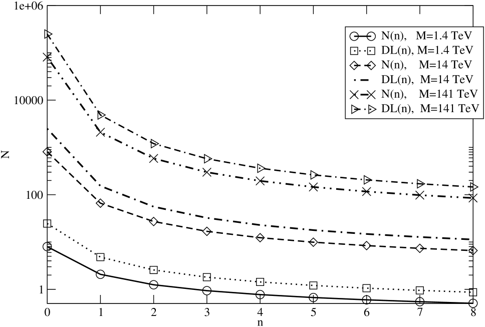
Figure 1: Multiplicities computed with Eq. (2) (N(n)) and Eq. (26) (DL(n)) for a varying number of extra dimensions $n$. DL(n) is the expression given in [15].

Since the number of elementary states becomes quite large as we raise the black hole mass compared to the (fixed) gravity scale, and given the (large) statistical fluctuations induced by the formation of the airshower, which reduce the dependence on the multiplicity formula used, we will adopt Eq. (26) in our simulations. Overall, in the massless approximation, the emission of the various species for a 3-brane is characterized by approximately $2\%$ into spin zero, $85\%$ into spin half and $13\%$ into spin one particles, with similar contributions also for the power emissivities. These numbers change as we vary the dimension of the brane (d) and so does the formula for the emissivities, since the number of brane degrees of freedom $(c_{i}(d))$ has to be recomputed, together with the integrals on the emission spectra $(f_{i}(d))$ [23].

The integration of the equation for the power spectrum, in the massless approximation, can be used to compute the total time of decay (assuming no mass evolution during the decay)

$$\tau\sim\frac{1}{M_{*}}\,\biggl{(}\frac{M_{BH}}{M_{*}}\biggr{)}^{(n+3)/(n+1)}\,$$ (28)

which implies that at an energy of approximately 1 TeV the decay time is of the order of $10^{-27}$ seconds. Therefore strong interaction effects and gravity effects appear to be widely separated and hadronization of the partons takes place after their crossing of the horizon. The black hole is assumed to decay isotropically (s-wave) to a set of $N$ elementary states, selected with equal probability from all the possible states available in the Standard Model. We mention that in most of the analysis presented so far [18, 17, 23] the (semiclassical) energy loss due to bulk emission has not been thoroughly analyzed. We will therefore correct our numerical studies by keeping into account some estimates of the bulk emission.

3 Modeling of the Black Hole Decay

The amount of radiation emitted by the black hole in the ED is viewed, by an observer living on the brane, as missing energy compared to the energy available at the time when the black hole forms. From the point of view of cosmic ray physics missing energy channels imply reduced multiplicities in the final air shower and modified lateral distributions, these two features being among the main observables of the cosmic ray event. However, since the initial energy of the original cosmic ray is reconstructed by a measurement of the multiplicities, an event of reduced multiplicity will simply be recorded as an event of lower energy. It is then obvious that an additional and independent reconstruction of the energy of the primary cosmic ray is needed in order to correctly identify the energy of these events.

In our study we will compute all the observables of the induced air shower using both the lab frame (LF) and the black hole frame (BHF) to describe the impact and the formation of the intermediate black hole resonance. Also, in the simulations that we will perform, the observation level at which we measure the properties of the air showers will be selected to take properly into account the actual position of a hypothetical experimental detector. The target of the first impact of mass $M$ is assumed to be a nucleon (or a quark) at rest in the atmosphere and the center of mass energy, corrected by emission loss in the bulk, is made promptly available for an instantaneous black hole formation and decay. We will also assume that the energy $E_{1}$ of the incoming primary varies over all the highest part of the cosmic ray spectrum, from $10^{15}$ eV up to $10^{20}$ eV.

We denote by $\beta$ the speed of the black hole in the lab frame. In our notations, $E^{*}$ is the typical energy of each elementary state in the decay products (parton, lepton) in the BH frame and $P^{*}$ is its corresponding momentum.

We will assume that a black hole decays “democratically” into all the possible partonic states, proportionally to the number of Standard Model states which are available to it at a given energy.

The energy per partonic channel will be appropriately weighted and we will assume that each parton $(f)$ will decay into a final state hadron $h$ (carrying a fraction $x$ of the original momentum), with a probability distribution given by the corresponding fragmentation function $D_{f}^{h}(x,Q^{2})$, which is evolved from some low energy input scale $Q_{0}$ up to the relevant scale characterizing the decay. This is given by the available energy per fundamental state, equally distributed among all the states.

The quantification of the injection spectrum involves a computation of the relevant probabilities for the formation of all the possible hadronic/leptonic states prior to the simulation of the air shower. Let’s briefly elaborate on this.

To move from the parton level to hadron level, we let $D_{q}^{h}(x,Q^{2})$, $D_{\overline{q}}^{h}(x,Q^{2})$, and $D_{g}^{h}(x,Q^{2})$ be the fragmentation functions of $N_{F}$ quarks $q$, antiquarks $\overline{q}$, and of the gluon $g$, respectively, into some hadron $h$ with momentum fraction $x$ at the scale $Q$. From the fragmentation functions we obtain, for each hadron $h$, the mean multiplicity of the corresponding s-wave and the corresponding average energy and momentum. Specifically we obtain

$$<D_{h}> = \sum_{f}\int_{z_{min}}^{1}dz\,D_{f}^{h}(z,Q^{2})$$ (29)

for the probability of producing a hadron $h$, and

$$E^{*}_{h} = \sum_{f}\int_{z_{min}}^{1}z\,dz\,D_{f}^{h}(z,Q^{2})$$ (30)

for the average energy of the same hadron. We recall that $z_{min}$ is the minimal fraction of energy a hadron $(h)$, of mass $m_{h}$, can take at a scale $Q$, and can be defined as $z_{min}=m_{h}/(Q/2)$. In practical applications one can take the nominal value $z_{min}=0.05$ for every hadron, without affecting much the mean multiplicities and the related probabilities. This implies that

$$<D_{r}^{h}>+\sum_{f}<D_{f}^{h}>+<D_{g}^{h}>+<D_{\gamma}^{h}>\equiv\textrm{Pr}_{h}\\$$

together with the condition $\sum_{h}\textrm{Pr}_{h}=1$, where the sum runs over all the types of hadrons allowed by the fragmentation. In all the equations above, the fragmentation takes place at the typical scale $Q=E/N$, scale at which the moments are computed numerically. For the identification of the probabilities it is convenient to organize the 123 fundamental states of the Standard Model into a set of flavour states $(q_{f})$, with $f$ running over all the flavours except for the top quark, where in $(q_{f})$ we lump antiquark states and color states, plus some additional states. The weight of the $(q_{f})$ set is $p_{f}=2\times 2\times 3/123$, where the factors 2 and 3 refer to spin, quark-antiquark degeneracy and color. It is worth to recall that quark and antiquark states of the same flavour have equal fragmentation functions in all the hadrons, and this justifies the $q/\bar{q}$ degeneracy of the set. The additional states are the gluon (g) with a weight $p_{g}=2\times 8/123$, the photon $(\gamma)$, with a weight $p_{\gamma}=2/123$ and the remaining states $(r)$ in which we lump all the states which have been unaccounted for, whose probabilities $p_{r}$ are computed by difference. These include the top and the antitop $(12/123)$, the W’s and Z $(9/123)$ and the leptons $(24/123)$. The fragmentation functions into hadrons, corresponding to these states, $<D_{r}^{h}>$ are computed by difference from the remaining ones $<D_{g}^{h}>$, $<D_{f}^{h}>$ and $<D_{\gamma}^{h}>$, which are known at any scale $Q$ from the literature. Beside the favour index $f=u,d,c,s,b$, introduced above, we introduce a second index $i$ running over the $(r)$ states, the photon and the gluons $(i=g,\gamma,r)$.

The probability of generating a specific sequence of $N$ states in the course of the evaporation of the black hole is then given by a multinomial distribution of the form

$$f(n_{f},n_{i},p_{f},p_{i})={N!\over\prod_{f}n_{f}!\prod_{i}n_{i}!}\prod_{f}p_{f}^{n_{f}}\prod_{i}{p_{i}}^{n_{i}}$$ (31)

which describes a typical multi-poissonian process with $N$ trials. Notice that, to ensure proper normalization, we need to require that

$$\prod_{i}n_{i}! = n_{g}!n_{\gamma}!n_{r}!$$ (32)

$$= n_{g}!n_{\gamma}!(N-\sum_{f}n_{f}-n_{g}-n_{\gamma})!$$

The computation of the cumulative probabilities to produce any number of hadrons of type $h$ by the decay of the black hole are obtained from the multinomial distribution multiplied by the fragmentation probabilities of each elementary state into $(h)$ and summing over all the possible sequences

$$\textrm{Pr}_{\textrm{cum h}}\equiv\sum_{n_{f},n_{i}}{N!\over\prod_{f}n_{f}!\prod_{i}n_{i}!}\prod_{f}\left(p_{f}<D_{f}^{h}>\right)^{n_{f}}\prod_{i}\left(p_{i}<D_{i}^{h}>\right)^{n_{i}}.$$ (33)

A possible way to compute $\textrm{Pr}_{\textrm{cum h}}$ when $N$ is large is to multiply the multinomial distribution by a suppression factor $\textrm{Exp}[{-\Lambda(\sum_{i}n_{i}+\sum_{f}n_{f}-N)}]$, with $\Lambda$ a very large number, and interpret this factor as a Boltzmann weight, as in standard Monte Carlo computations of the partition function for a statistical system. Simulations can be easily done by a Metropolis algorithm and the configurations of integers selected are those for which the normalization condition $N=\sum_{i}n_{i}+\sum_{f}n_{f}$ is satisfied. In our case, since we are interested only in the mean number of hadrons produced in the decay and in their thermal spectrum, the computation simplifies if we average over all the relevant configurations.

4 Fragmentation and the Photon Component

The evolution with $Q^{2}$ of the fragmentation functions is conveniently formulated in terms of the linear combinations

$$D_{\Sigma}^{h}(x,Q^{2}) = \sum_{i=1}^{N_{F}}\left(D_{q_{i}}^{h}(x,Q^{2})+D_{\overline{q}_{i}}^{h}(x,Q^{2})\right)\hskip 2.84544pt,$$ (34)

$$D_{(+),i}^{h}(x,Q^{2}) = D_{q_{i}}^{h}(x,Q^{2})+D_{{\overline{q}},i}^{h}(x,Q^{2})-\frac{1}{N_{F}}D_{\Sigma}^{h}(x,Q^{2})\hskip 2.84544pt,$$ (35)

$$D_{(-),i}^{h}(x,Q^{2}) = D_{q_{i}}^{h}(x,Q^{2})-D_{{\overline{q}},i}^{h}(x,Q^{2})\hskip 2.84544pt,$$ (36)

as for these the gluon decouples from the non–singlet $\scriptstyle(+)$ and the asymmetric $\scriptstyle(-)$ combinations, leaving only the singlet and the gluon fragmentation functions coupled;

$$Q^{2}\frac{d}{dQ^{2}}D_{(+),i}^{h}(x,Q^{2}) = \left[P_{(+)}\left(\alpha_{s}(Q^{2})\right)\otimes D_{(+),i}^{h}(Q^{2})\right](x)\hskip 2.84544pt,$$ (37)

$$Q^{2}\frac{d}{dQ^{2}}D_{(-),i}^{h}(x,Q^{2}) = \left[P_{(-)}\left(\alpha_{s}(Q^{2})\right)\otimes D_{(-),i}^{h}(Q^{2})\right](x)\hskip 2.84544pt,$$ (38)

$$Q^{2}\frac{d}{dQ^{2}}D_{\Sigma}^{h}(x,Q^{2}) = \left[P_{\Sigma}\left(\alpha_{s}(Q^{2})\right)\otimes D_{\Sigma}^{h}(Q^{2})\right](x)$$ (39)

$$\hskip 28.45274pt+2N_{F}\left[P_{q\to G}\left(\alpha_{s}(Q^{2})\right)\otimes D_{G}^{h}(Q^{2})\right](x)\hskip 2.84544pt,$$

$$Q^{2}\frac{d}{dQ^{2}}D_{G}^{h}(x,Q^{2}) = \frac{1}{2N_{F}}\left[P_{G\to q}\left(\alpha_{s}(Q^{2})\right)\otimes D_{\Sigma}^{h}(Q^{2})\right](x)$$ (40)

$$\hskip 28.45274pt+\left[P_{g\to g}\left(\alpha_{s}(Q^{2})\right)D_{g}^{h}(Q^{2})\right](x)\hskip 2.84544pt.$$

The kernels that appear in the equations above are defined by

$$P_{(+)}\left(x,\alpha_{s}(Q^{2})\right) = P_{q\to q}^{V}\left(x,\alpha_{s}(Q^{2})\right)+P_{q\to\overline{q}}^{V}\left(x,\alpha_{s}(Q^{2})\right)\hskip 2.84544pt,$$ (41)

$$P_{\Sigma}\left(x,\alpha_{s}(Q^{2})\right) = P_{(+)}\left(x,\alpha_{s}(Q^{2})\right)+2N_{F}P_{q\to q}^{S}\left(x,\alpha_{s}(Q^{2})\right)\hskip 2.84544pt,$$ (42)

$$P_{(-)}\left(x,\alpha_{s}(Q^{2})\right) = P_{q\to q}^{V}\left(x,\alpha_{s}(Q^{2})\right)-P_{q\to\overline{q}}^{V}\left(x,\alpha_{s}(Q^{2})\right),$$ (43)

with $\alpha_{s}(Q^{2})$ being the QCD coupling constant. In the perturbative expansion of the splitting functions,

$$P(x,\alpha_{s}(Q^{2}))=\frac{\alpha_{s}(Q^{2})}{2\pi}P^{(0)}(x)+\left(\frac{\alpha_{s}(Q^{2})}{2\pi}\right)^{2}P^{(1)}(x)+{\cal O}\left(\left(\frac{\alpha_{s}(Q^{2})}{2\pi}\right)^{3}\right).$$ (44)

The timelike kernels that we use are given by

$$P_{q\to q}^{V,(0)}(x) = C_{F}\left[\frac{3}{2}\delta(1-x)+2\left(\frac{1}{1-x}\right)_{+}-1-x\right]\hskip 2.84544pt,$$ (45)

$$P_{q\to\overline{q}}^{V,(0)}(x) = P_{q\to q}^{S,(0)}(x)=0\hskip 2.84544pt,$$ (46)

$$P_{q\to G}^{(0)}(x) = C_{F}\left[\frac{1+(1-x)^{2}}{x}\right]\hskip 2.84544pt,$$ (47)

$$P_{q\to q}^{(0)}(x) = 2N_{F}T_{R}\left[x^{2}+(1-x)^{2}\right]\hskip 2.84544pt,$$ (48)

$$P_{G\to G}^{(0)}(x) = \left(\frac{11}{6}N_{C}-\frac{2}{3}N_{F}T_{R}\right)\delta(1-x)$$ (49)

$$\hskip 28.45274pt+2N_{C}\left[\left(\frac{1}{1-x}\right)_{+}+\frac{1}{x}-2+x-x^{2}\right]\hskip 2.84544pt.$$

The formal solution of the equations is given by

$$D_{a}^{h}(x,Q^{2})=D_{a}^{h}(x,Q_{0}^{2})+\int_{0}^{\log(Q^{2}/Q_{0}^{2})}d\log(Q^{2}/Q_{0}^{2})\frac{\alpha_{s}(Q^{2})}{2\pi}\sum_{b}\left[P_{a\to b}(\alpha_{s}(Q^{2}))\otimes D_{b}^{h}(Q^{2})\right]$$ (50)

where $Q_{0}$ is the starting scale of the initial conditions, given by $D(x,Q_{0}^{2})$. At leadiong order in $\alpha_{s}$, we solve this equation using a special ansatz

$$D_{f}^{h}(x,Q^{2})=\sum_{n}{A_{n}(x)\over n!}\log\left({\alpha_{s}(Q^{2})\over\alpha_{s}(Q_{0}^{2})}\right)^{n}$$ (51)

and generating recurrence relations at the $n+1-th$ order for the $A_{n+1}$ coefficients in terms of the $A_{n}$ [36]. It is easy to see that this corresponds to the numerical implementation of the formal solution

$$D_{f}^{h}(x,Q^{2})={\it{Exp}}\left(tP\otimes\right)D_{f}^{h}(x,Q_{0}^{2})$$ (52)

with $t=\left(\alpha_{s}(Q^{2})/\alpha_{s}(Q_{0}^{2})\right)$, where the exponential is a formal expression for an infinite iteration of convolution products. We show in Figures 2-4 results for some of the fragmentation functions into pions, kaons and protons computed for a typical parton scale of 200 GeV.

Figure 2: Fragmentation functions into $\pi^{\pm}$ at $200\,\textrm{GeV}$.

Figure 3: Fragmentation functions into $K^{\pm}$ at $200\,\textrm{GeV}$.

Figure 4: Fragmentation functions into $p/\overline{p}$ at $200\,\textrm{GeV}$.

The photon contributions to the decay of the black hole is treated separately. The evolution equation for the fragmentation functions of photons and parton fragmentation into photon $D_{\gamma}^{\gamma}(x,Q^{2}),\,\,D_{q}^{\gamma}(x,Q^{2})$ satisy at leading order in $\alpha_{\rm{em}}$ (the QED fine structure constant) and $\alpha_{s}$ (the QCD coupling), the evolution equations [49]

$$\frac{\textrm{d}D_{\gamma}^{\gamma}(x,Q^{2})}{\textrm{d}\ln Q^{2}}=\frac{\alpha}{2\pi}P_{\gamma\rightarrow\gamma}(x)\otimes D_{\gamma}^{\gamma}(x,Q^{2})$$ (53)

which can be integrated with the initial conditions $D_{\gamma}^{\gamma}(x,Q^{2})=\delta(1-x)$, and

$$\frac{\textrm{d}D_{q}^{\gamma}(x,Q^{2})}{\textrm{d}\ln Q^{2}}=\frac{\alpha}{2\pi}P_{\gamma\rightarrow\gamma}(x)\otimes D_{\gamma}^{\gamma}(x,Q^{2})$$ (54)

which can also be integrated with the result [50]

$$D_{\gamma/q}(x,Q^{2})=\frac{\alpha}{2\pi}P_{q\rightarrow\gamma}(x)\ln\frac{Q^{2}}{Q_{0}^{2}}+D_{q}^{\gamma}(x,Q_{0}^{2}).$$ (55)

In Eq. (55) the second term is termed the hadronic boundary conditions, which come from an experimental fit, while the first term is the pointlike contributions, which can be obtained perturbatively. In [51] a leading order fit was given

$$D_{q}^{\gamma}(x,Q_{0}^{2})=\frac{\alpha}{2\pi}\left[-\,P_{q\rightarrow\gamma}(x)\ln(1-x)^{2}-13.26\right]$$ (56)

at the starting scale $Q_{0}=0.14$ GeV. The kernels in these cases are given by simple modifications of the ordinary QCD kernels, for instance $P_{q\rightarrow\gamma}(x)=e_{q}^{2}/C_{F}P_{q\rightarrow g}(x)$ [49].

For the fragmentation function of quarks to photons with virtuality $M_{\gamma}$, the perturbative result is given in [52]

$$D_{\gamma/q}(x,Q^{2},M_{\gamma}^{2})=e_{q}^{2}\frac{\alpha}{2\pi}\left[\frac{1+(1-x)^{2}}{x}\ln\frac{xQ^{2}}{M_{\gamma}^{2}}-x\left(1-\frac{P^{2}}{xQ^{2}}\right)\right],$$ (57)

where $P^{2}$ is the virtuality of the photon. The gluon to photon transitions are neglected, since $P_{g\rightarrow\gamma}$ vanishes in leading order.

We recall that each elementary state emitted is characterized by an average energy given by $\left\langle\varepsilon\right\rangle=M_{BH}/\left\langle N\right\rangle$.

The leptonic component $e^{\pm}$, $\mu^{\pm}$, produced by the decay is left unaltered and provides an input for the air shower simulator as soon as these particles cross the horizon. The $\tau^{\pm}$s are left to decay into their main channels, while the hadronization of the $u,\,d,\,s,\,c$ quarks and the gluons is treated with our code, that evolves the fragmentation functions to the energy scale $\left\langle\varepsilon\right\rangle$. The top ($t$) quark is treated consistently with all its fundamental decays included; hadronization of the $b$ quark is treated with suitable fragmentation functions and also involves a suitable evolution. As we vary $M_{BH}$ and we scan over the spectrum of the incoming cosmic rays the procedure is repeated and rendered automatic by combining in a single algorithm all the intermediate steps. Tables 1 and 2 contain the results of a renormalization group analysis of the fragmentation functions for all the partons (except the top quark), where we show both the intial conditions at the input scale, whose lowest value is $Q=1.414$ GeV, and the results of the evolution, at a final scale of $Q=200$ GeV, the initial set being taken from ref. [37].

	$\pi^{\pm}$	$\pi^{0}$	$K^{\pm}$	$K^{0}/\overline{K}^{0}$	$p/\overline{p}$	$n/\overline{n}$
u	$0.451$	$0.226$	$0.048$	$0.174$	$0.067$	$0.034$
	$0.463$	$0.231$	$0.084$	$0.252$	$0.070$	$0.035$
d	$0.451$	$0.226$	$0.174$	$0.048$	$0.034$	$0.067$
	$0.463$	$0.231$	$0.252$	$0.084$	$0.035$	$0.070$
s	$0.391$	$0.195$	$0.068$	$0.068$	$0.139$	$0.139$
	$0.295$	$0.147$	$0.084$	$0.084$	$0.108$	$0.108$
c	$0.329$	$0.165$	$0.167$	$0.167$	$0.085$	$0.085$
	$0.309$	$0.155$	$0.194$	$0.194$	$0.071$	$0.071$
b	$0.438$	$0.219$	$0.129$	$0.129$	$0.042$	$0.042$
	$0.324$	$0.162$	$0.115$	$0.115$	$0.041$	$0.041$
g	$0.303$	$0.152$	$0.253$	$0.253$	$0.020$	$0.020$
	$0.807$	$0.404$	$0.317$	$0.317$	$0.034$	$0.034$

Table 1: Initial conditions. For each couple of parton and hadron, the upper number in the box is the probability for the parton $f$ to hadronize into the hadron $h$, $\left(\int_{z_{min}}^{1}D_{f}^{h}(z,Q)dz\right)/\sum_{h^{\prime}}\left(\int_{z_{min}}^{1}D_{f}^{h^{\prime}}(z,Q)dz\right)$, while the lower number is the average energy fraction of $h$, $\int_{z_{min}}^{1}zD_{f}^{h}(z,Q)dz$. In this table the energy of the parton is $Q=1.414\,\textrm{GeV}$ for $u$, $d$, $s$ and $g$, $Q=2m_{c}=2.9968\,\textrm{GeV}$ for $c$ and $Q=2m_{b}=9.46036\,\textrm{GeV}$ for the $b$ quark, generated via the set of ref. [37]

$Q=200\,\textrm{GeV}$	$\pi^{\pm}$	$\pi^{0}$	$K^{\pm}$	$K^{0}/\overline{K}^{0}$	$p/\overline{p}$	$n/\overline{n}$
u	$0.446$	$0.223$	$0.079$	$0.166$	$0.053$	$0.033$
	$0.385$	$0.193$	$0.077$	$0.178$	$0.047$	$0.027$
d	$0.446$	$0.223$	$0.166$	$0.079$	$0.033$	$0.053$
	$0.385$	$0.193$	$0.178$	$0.077$	$0.027$	$0.047$
s	$0.425$	$0.213$	$0.093$	$0.093$	$0.088$	$0.088$
	$0.295$	$0.147$	$0.077$	$0.077$	$0.070$	$0.070$
c	$0.371$	$0.185$	$0.158$	$0.158$	$0.064$	$0.064$
	$0.295$	$0.147$	$0.150$	$0.150$	$0.051$	$0.051$
b	$0.431$	$0.216$	$0.132$	$0.132$	$0.045$	$0.045$
	$0.292$	$0.146$	$0.101$	$0.101$	$0.036$	$0.036$
g	$0.428$	$0.214$	$0.135$	$0.135$	$0.044$	$0.044$
	$0.577$	$0.289$	$0.175$	$0.175$	$0.057$	$0.057$

Table 2: For each couple of parton/hadron, the first number is the probability of fragmentation of the parton $f$ into the hadron $\left(\int_{z_{min}}^{1}D_{f}^{h}(z,Q)dz\right)/\sum_{h^{\prime}}\left(\int_{z_{min}}^{1}D_{f}^{h^{\prime}}(z,Q)dz\right)$, while the second is the average energy fraction of $h$, $\int_{z_{min}}^{1}zD_{f}^{h}(z,Q)dz$. The energy of the parton is $Q=200$ GeV.

This concludes the computation of the probabilities for each hadron/lepton present in the decay products of the mini black hole. It is reasonable to assume that these particles will be produced spherically, since higher angular momenta are suppressed by the corresponding centrifugal barrier. However, the analysis of the shower profile has to be performed in the lab frame. This requires the transformation of the initial configurations above to the laboratory frame, which is exactly what is discussed next.

5 Sphericity and Boost

The transformation from the black hole frame (BHF) to the laboratory frame (LF) is performed by a Lorentz boost with speed $\beta$, the speed of the black hole in the LF. Assuming that the black hole is produced in the collision of a primary of energy $E_{1}$ in the LF and negligible mass compared to $E_{1}$, with a parton of mass $M$ in the atmosphere, one obtains $\beta=E_{1}/(E_{1}+M)$. A spherical distribution of a particular particle of mass $m$ among the decay products in the BHF is transformed to an elliptical one, whose detailed form is conveniently parametrized by

$$g^{*}={\beta\over\beta^{*}}=\frac{1-\frac{M}{E_{1}+M}}{\left(1-{{m^{2}}\over{E^{*2}}}\right)^{1/2}}$$ (58)

where $\beta^{*}=P^{*}/E^{*}$ is the speed of this particle in the BHF, the ratio of its BHF momentum and energy. Figure 5 depicts the relevant kinematics. A particle emitted in the direction $\theta^{*}$ in the BHF, is seen in the direction $\theta$ in the LF, with

$$\tan\theta=\sqrt{1-\beta^{2}}\frac{\sin\theta^{*}}{g^{*}+\cos\theta^{*}}.$$ (59)

For values of $g^{*}\geq 1$ the shape of the 1-particle distribution in the LF is characterized by a maximum angle of emission

$$|\tan\theta_{max}|=\sqrt{\frac{1-\beta^{2}}{g^{*2}-1}}\,,$$ (60)

which for $g^{*}=1$ is equal to $90^{o}$. Only for $g^{*}<1$ there is backward emission in the LF.

Figure 5: An s-wave distribution in the BHF is transformed in the detector frame to an elliptical one, whose detailed shape depends on the value of $g^{*}$

As a relevant example, let us consider the case of a hadron of mass $m=1$ GeV and energy $E^{*}=100$ GeV emitted by a black hole, formed by an initial primary of energy $E_{1}=1000$ TeV, which hit a quark of mass $M\sim 10$MeV to form a black hole. The gives $g^{*}=1.00005$ and the corresponding maximum angle in the LF is $\theta_{max}\simeq\tan\theta_{max}=1.4\times 10^{-2}$, giving an angular opening of the decay products of about 2 degrees.

As shown in Figure 5, for $g^{*}>1$, which is relevant for our purposes, the mapping from $\theta^{*}$ to $\theta$ is not one to one. In a given direction $\theta$ in the LF, one receives particles emitted in two different directions $\theta^{*\pm}$ in the BHF. They satisfy [48]

$$\frac{d\cos\theta^{*\pm}}{d\cos\theta}=\left(\frac{P^{\pm}}{P^{*}}\right)^{2}\frac{1}{\left(\pm\cos\theta\sqrt{K}\right)}$$ (61)

where

$$K=1+\gamma^{2}(1-{g^{*}}^{2})\tan^{2}\theta,$$ (62)

and with the momenta $P^{\pm}$ and energies $E^{\pm}$ of the two branches given by

$$P^{\pm}={P^{*}\cos\theta(g^{*}\pm\sqrt{K})\over\gamma(1-v^{2}\cos^{2}\theta)}.$$ (63)

and

$$E^{\pm}=\frac{m\left(\gamma^{*}\pm v\cos\theta\left(v^{*2}\gamma^{*2}-v^{2}\gamma^{2}\sin^{2}\theta\right)^{1/2}\right)}{\gamma(1-v^{2}\cos^{2}\theta)}$$ (64)

respectively. In the above formulas $\gamma^{-1}=\sqrt{1-\beta^{2}}$, $v(v^{*})$ is the speed of the hadron in the LF (BHF), and $(\gamma^{*})^{-1}=m/E^{*}_{h}=\sqrt{1-v^{*2}}$. For massless final state particles, in particular, these relations become

$$P=E={P^{*}\over\gamma(1-\cos\theta)}$$ (65)

and reduce to the familiar Doppler formula when $\theta=0$.

The probability distribution $W_{h}^{*}(\cos\theta^{*},\phi)$ of a hadron (h) as a function of the direction $\Omega=(\cos\theta^{*},\phi)$ in the BHF, assumed spherically symmetric and normalized to the total probability $Pr_{h}$ of detecting this hadron among the decay products with $N$ elementary states, is

$$W_{h}^{*}(\cos\theta^{*})={\textrm{Pr}_{h}\over 2}.$$ (66)

The corresponding one in the LF is

$$W_{h}(\cos\theta)=\sum_{\pm}\frac{d\cos\theta^{*\pm}}{d\cos\theta}\,W^{*}_{h}(\cos\theta^{*\pm})\,.$$ (67)

In the special case $g^{*}=1$, the probability distribution simplifies to

$$W_{h}(\cos\theta)=2\textrm{Pr}_{h}{\cos\theta\over\gamma^{2}(1-\beta^{2}\cos\theta^{2})^{2}}\,,$$ (68)

peaked in the forward direction, symmetric around the maximum value, obtained for $\theta=0$ and equal to $2\gamma^{2}$, while the momentum distribution is

$$P(\theta)=m{\beta\gamma^{*}\cos\theta\over\gamma(1-\beta^{2}\cos\theta^{2})}\,.$$ (69)

As we have already mentioned, the structure of the partonic event (and, similarly, of the hadronic event after fragmentation) is characterized by the formation of an elliptical distribution of partons, strongly boosted toward the detector along the vertical direction. Each uniform (s-wave) distribution is strongly elongated along the arrival direction (due to the large speed of the black hole along this direction) and is characterized by two sub-components ($W^{\pm}$), identified by a $\pm$ superscript. Their sum is the total probability distribution given in (61). The “+” momentum component is largely dominant and strongly peaked around the vertical direction with rather small opening angles and this behaviour can be analyzed numerically with its $N$ dependence. In the explicit identification of the two independent distributions $\pm$ in terms of the opening angle $\theta$, as measured in the LF, we use the relations

$$W^{\pm}(\theta)=\frac{1}{2}W^{\pm}(\cos\theta^{*})\mid{d\cos(\theta^{*})\over d\cos\theta}^{\pm}\mid\sin\theta,$$ (70)

where we have introduced a factor of 1/2 for a correct normalization of the new distribution in the $\theta$ variable. In Figures 7 and 7 we show the structure of these distributions in the LF. Both are characterized by a very small opening angle ($\theta$) with respect to the azimuthal direction of the incoming cosmic ray, $W^{+}$ being the dominant one. Two similar plots (Figures 9 and 9) illustrate the two components $P^{\pm}$ as functions of the same angle.

Figure 6: Plot of the $W^{+}$ branch of the probability distribution for an incoming energy of the cosmic ray $E_{1}=10^{8}$ GeV and for various values of $N$ of the elementary partonic states emitted during the decay of the black hole

Figure 7: Same plot as above but for the $W^{-}$ branch of the distribution

Figure 8: Plot of the $P^{+}$ branch of the momentum distribution in eV for an incoming energy of the cosmic ray $E_{1}=10^{8}$ GeV and for various values of $N$ of the elementary partonic states emitted during the decay of the black hole

Figure 9: Same plot as above but for the $P^{-}$ branch of the momentum distribution

One can easily check that we can now integrate symmetrically on both distributions to obtain the correct normalization (to $\textrm{Pr}_{h}$) for a given hadron (or parton)

$$\int_{-\theta_{max}}^{\theta_{max}}W^{\pm}(\theta)d\theta=\int_{-{\theta_{1}}^{*}}^{{\theta_{1}}^{*}}W^{+}(\theta)d\theta+\int_{{\theta_{1}}^{*}}^{\pi}W^{-}(\theta)d\theta+\int_{-\pi}^{{-\theta_{1}}^{*}}W^{-}(\theta)d\theta={\textrm{Pr}_{h}}$$ (71)

or, equivalently, using $\cos\theta$ as a distribution variable

$$W^{\pm}(cos\theta)=W^{\pm}(\cos\theta^{*})\mid{d\cos\theta^{*}\over d\cos\theta}^{\pm}\mid\sin\theta$$ (72)

with

$$\int_{cos\theta_{max}}^{1}W^{\pm}(\cos\theta)d\cos\theta=\int_{\cos{\theta_{1}}^{*}}^{1}W^{+}(\cos\theta^{*})d\ cos\theta^{*}+\int_{-1}^{\pi}W^{-}(\cos\theta^{*})d\cos\theta^{*}={\textrm{Pr}_{h}}$$ (73)

and ${\theta^{*}}_{1}$ obtained from (60).

6 Air Shower Simulations

The simulation of the events is performed at the last stage, using an air shower simulator. We have used CORSIKA [29] with appropriate initial conditions on the spectrum of the incoming particles in order to generate the full event measured at detector level. In most of the simulations we have assumed that the first impact takes place in the lower part of the atmosphere, not far from the level of the detector, at a varying altitude. The reason is that one of our interests is the investigation of the possibility that the Centauro events may be related to evaporating mini black holes, formed by the collision of weakly interacting particles (e.g. neutrinos) which penetrate the atmosphere. Of course, we have simulated events happening at higher altitudes as well. We have performed two separate sets of simulations, the first set being benchmark events with an “equivalent” proton replacing the neutrino-nucleon event, colliding at the same height, the second being the signal event, i.e. the black hole resonance. The difference between the first and the second set is attributed to the different components of the final state prior to the development of the air shower.

We compute the average number of particles produced in the process of BH evaporation using the formula

$$M_{BH}=E_{CM}f_{n}$$ (74)

where $E_{CM}$ is the energy in the center of mass frame in the neutrino-nucleon collision and $f_{n}$ is the fraction of $E_{CM}$ that is bound into the black hole as a function of the number $n$ of extra-dimensions. Numerical values for $f_{n}$ in head-on collisions are taken from Ref. [53] and reported in Table 3.

$n$	$f_{n}$
0	$0.70711$
1	$0.66533$
2	$0.63894$
3	$0.62057$
4	$0.60696$

Table 3: Fraction $f_{n}$ of $E_{CM}$ that is bound into the black hole as a function of the number $n$ of extra-dimension in head-on collisions.

The overall shower, defined as the superposition of the various sub-components, develops according to an obvious cylindrical symmetry around the vertical z-axis near the center. We assume in all the studies that the incoming primary undergoes a collision with a nucleon in the atoms of the atmosphere at zero zenith with respect to the plane of the detector.

The model of the atmosphere that we have adopted consists of $N_{2}$, $O_{2}$ and $Ar$ with the volume fractions of $78.1\%$, $21.0\%$ and $0.9\%$ [54]. The density variation of the atmosphere with altitude is modeled by 5 layers. The pressure $p$ as a function of the altitude $h$ is given by

$$p(h)=a_{i}+b_{i}\exp(-h/c_{i}),\quad i=1,\ldots,4$$ (75)

in the lower four layers and by

$$p(h)=a_{5}-h\frac{b_{5}}{c_{5}}$$ (76)

in the fifth layer.

The $a_{i}$, $b_{i}$, $c_{i}$ parameters, that we report in Table 4, are those of the U.S. standard atmospheric model [29]. The boundary of the atmosphere in this model is defined at the height $112.8\,\textrm{km}$, where the pressure vanishes. In Figure 10 we show a plot of the pressure ($p=X_{v}$, also called vertical depth) as a function of the height.

Layer $i$	Altitude $h$ [km]	$a_{i}\,[\textrm{g}/\textrm{cm}^{2}]$	$b_{i}\,[\textrm{g}/\textrm{cm}^{2}]$	$c_{i}\,[\textrm{cm}]$
1	$0\ldots 4$	$-186.5562$	$1222.6562$	$994186.38$
2	$4\ldots 10$	$-94.919$	$1144.9069$	$878153.55$
3	1$0\ldots 40$	$0.61289$	$1305.5948$	$636143.04$
4	$40\ldots 100$	$0.0$	$540.1778$	$772170.16$
5	$>100$	$0.01128292$	$1$	$10^{9}$

Table 4: Parameters of the U.S. standard atmosphere.

Figure 10: Pressure versus altitude for the U.S. standard atmosphere model.

This is defined via the integral

$$X_{v}=\int_{h}^{\infty}\rho(h^{\prime})dh^{\prime}$$ (77)

of the atmospheric density $\rho(h)$ for zero zenith angle, while the corresponding slant depth is given by

$$X=\int_{l}^{\infty}\rho\left(l\cos\theta+\frac{1}{2}\frac{l^{2}}{R_{T}}\sin^{2}\theta\right)$$ (78)

for a zenith angle $\theta$ and $R_{T}$ is the radius of the earth.

To put into perspective our Monte Carlo study it is convenient to briefly summarize the basic features of the theory of cascades on an analytical ground. The theory consists of the system of transport equations [55, 56] for the numbers $N_{n}(E,X)$ of particles of type $n$ with energy $E$ at height $X$

$$\frac{dN_{n}(E,X)}{dX}=-\frac{N_{n}(E,X)}{\lambda_{n}(E)}-\frac{1}{c\tau_{n}\gamma\rho_{\mathrm{Air}}}N_{n}(E,X)~{},$$ (79)

where $\lambda_{n}(E)$ is their interaction length, $\tau_{n}$ is their lifetime and $\gamma$ the Lorentz-factor corresponding to their given energy. In the simple case of an isothermal atmosphere $\rho_{\mathrm{Air}}=\rho_{0}\exp(-h/h_{0})=X/h_{0}$, at a scale height $h_{0}$

$$\frac{dN_{n}(E,X)}{dX}=-\frac{N_{n}(E,X)}{\lambda_{n}(E)}-\frac{1}{d_{n}}N_{n}(E,X)$$ (80)

where $d_{n}$ is their decay length, defined by

$$\frac{1}{d_{n}}=\frac{mc^{2}h_{0}}{Ec\tau_{n}X}.$$ (81)

Particles produced at higher energies are also accounted for by an additional term in the cascade

$$\frac{\partial N_{n}(E,X)}{\partial X} = -N_{n}(E,X)\left[\frac{1}{\lambda_{n}(E)}+\frac{1}{d_{n}(E)}\right]$$

$$+\sum_{m}\int_{E}^{E^{max}}N_{m}(E^{\prime},X)\left[\frac{W_{mn}(E^{\prime},E)}{\lambda_{m}(E^{\prime})}\right.$$

$$\,\,\,\,\,\,\,\,\,\,\,\,\,\,\,\left.+\frac{1}{d_{n}(E^{\prime})}D_{mn}(E^{\prime},E)\right]dE^{\prime}~{}~{},$$

describing the change in the number of particles of type $n$ due to particles of type $m$ by interaction or decay, integrated over an allowed interval of energy. The functions $W_{mn}(E^{\prime},E)$ are the energy-spectra of secondary particles of type $n$ in a collision of particle $m$ with an air-molecule, while $D_{mn}(E^{\prime},E)$ are the corresponding decay-functions. The advantage of a transport equation compared to a Monte Carlo is, that it provides a rather simple analytical view of the development of the cascade across the atmosphere. Most common in the study of these equations is to use a factorized ansatz for the solution $N(E,X)=A(E)B(X)$, which assumes a scaling in energy of the transition functions [55]. In our case an analytical treatment of the cascade corresponds to the boundary condition

$$N_{n}(E,X_{0})=\textrm{Pr}_{n}(E)\,\delta(E-fM_{BH}/\langle N\rangle)$$ (83)

with $\textrm{Pr}_{n}(E)$ being the probability that the black hole decays into a specific state $n$. As we have already discussed above, these decays are uncorrelated and Eq. (83) is replicated for all the elementary states after hadronization. The emission probabilities $\textrm{Pr}_{n}(E)$ have been computed by us for a varying initial energy $E=fM_{BH}$ using renormalization group equations as described before, having corrected for energy loss in the bulk. The interactions in the injection spectrum of the original primaries at our $X_{0}$ ($X_{0}=517$ g/cm²) has been neglected since this is not implemented in CORSIKA. The showers have been performed independently and the results of the simulations have been statistically superimposed at the end with multiplicities computed at detector level ($X_{1}=553$ g/cm²). We have kept the gravity scale $M_{*}$ constant at 1 TeV and varied the mass of the black hole according to the available center of mass energy $E$. As we have already discussed in the previous sections, as a benchmark process we have selected a proton-air impact at the same $X_{0}$ with the boundary condition

$$N_{p}(E,X_{0})=\textrm{Pr}_{p}\delta(E-fM_{BH})$$ (84)

which occurs with probability 1 ($Pr_{p}=1$).

We are interested both in the behaviour of the multiplicities and in the lateral distributions of the cascades developed at detector level. For this purpose we have defined the opening of the conical shower after integration over the azimuthal angle, as in [27], and given the symmetry of the event, we plot only the distance from the center as a relevant parameter of the conical shower.

A varying number of extra dimensions $n=0,\,1,\ldots,4$ implies a different ratio for bulk-to-brane energy emission, a different average number of elementary decaying states and different energy distributions among these. We have varied the energy $E_{1}$ of the primary, thereby varying the mass of the black hole resonance, in the interval $10^{15}-10^{20}$  eV. The hadronization part of our code has been done by changing the $\textrm{Pr}_{h}(E)$ obtained from a numerical solution of the fragmentation functions separately for each value of the energy shared.

• Preliminary studies

  We start with the numerical study of the partial and total multiplicities of the various sub-components and of their lateral distributions in the benchmark event. The results for photons and leptons are shown in Figures 11 to 14 as functions of the altitude of the impact and for two different observation points at 4,500 m and 5,000 m, approximately the altitudes of the detectors at Pamir and Chacaltaya, respectively. These preliminary plots, based on actual simulations of a proton-to-air nucleus impact at $10^{15}$ eV, show a steady growth of the multiplicities of the secondaries as we raise the point of first impact above the detector.

  

  Figure 11: Benchmark event: Multiplicities of photons, $e^{\pm}$, $\mu^{\pm}$ at an observation level of 4500 m as a function of the altitude of the first impact.

  

  Figure 12: As in Figure 11, but at an observation level of 5000 m.

  

  Figure 13: Average radial opening of the shower of photons, $e^{\pm}$, $\mu^{\pm}$ at an observation level of 4500 m as a function of the altitude of proton’s first interaction.

  

  Figure 14: As in Fig. 13, but at an observation level of 5000m.

  The statistical errors in the simulations (80 uncorrelated events have been collected per point) are rather small, quite uniformly over all the altitudes of the impact, and indicate a satisfactory stability of the result. The positions of the detectors do not seem to have an appreciable impact on the characteristics of the secondaries. As for the lateral distributions we observe an increase in the opening of the showers with the event altitude, which is more enhanced for the muonic component and for the photons and less for the electrons and positrons. Also in this case the statistical fluctuations are rather small. On the basis of these results we have selected for the remaining simulations a first impact at 5,500 m and the observation (detector) level at 5,000 m. However, for comparison, we will also show later the results of a second set of simulations that have been performed with the first impact at 15,000 m.

• Choice of scales and corrections

  To compare standard and black holes events, we have selected a gravity scale of $M_{*}=1$TeV and varied the black hole mass, here taken to be equal to the available center of mass energy during the collision. Therefore, a varying $E_{1}$ is directly related to a varying $M_{\rm{BH}}$ and we have corrected, as explained above, for the energy loss into gravitational emission. Unfortunately, this can be estimated only heuristically, with bounds largely dependent on the impact parameter of the primary collision. A reasonable estimate may be of the order of $10-15\%$ [35]. Corrections related to emission in the bulk have also been included, in the way discussed in previous sections.

• Energy ratios: electromagnetic versus hadronic

  Not all observables are statistically insensitive to the natural fluctuations of the air showers. In the study of black hole versus standard (benchmark) events, the study of the ratios $N_{\rm{em}}/N_{\rm{hadron}}$ and $E_{\rm{em}}/E_{\rm{hadron}}$ have been proposed as a way to distinguish between ordinary showers and other extra-ordinary ones. Centauro events, for instance, have been claimed to be characterized by a rather small ratio of electromagnetic over hadronic energy deposited in the detectors, contrary to normal showers, in which this ratio is believed to be $E_{\rm{em}}/E_{\rm{hadron}}\sim 2$. Instead, as one can easily recognize from the results presented in Figures 15 and 16, the multiplicity ratio takes values in two different regimes. In the “band” of values $1-5$ for the case of the lower first impact and $100-160$ for the higher impact. The larger values of the band in this latter case are justified by the fact that the shower is far more developed, given the altitude of the impact, and therefore is characterized by an even more dominant electromagnetic component. The energy ratio, on the other hand can take small values, in agrement with the values observed in Centauros. However, notice that both the black hole and standard simulations show a complex pattern for these ratios and in addition they are characterized by large fluctuations for varying energy and number of extra dimensions.

  

  (a)

  

  (b)

  Figure 15: Ratio between $N_{em}$ (total multiplicity of photons and $e^{\pm}$) and $N_{had}$ (total multiplicity of everything else) as a function of $E_{1}$. The first interaction is kept fixed at $5500\,\textrm{m}$ (517 $g/cm^{2}$) (a), or at $15000\,\textrm{m}$ (124 $g/cm^{2}$) (b), and the observation level is $5000\,\textrm{m}$ (553 $g/cm^{2}$). We show in the same plot the benchmark (where the primary is a proton) and mini black holes with different numbers of extra-dimensions $n$.

  

  (a)

  

  (b)

  Figure 16: As in Figure 15, but this time we show the ratio between $E_{em}$ (total energy of photons and $e^{\pm}$) and $E_{had}$ (total energy of everything else) as a function of $E_{1}$.

  Furthermore, there does not seem to be a statistically significant difference in these observables between the benchmark event and the black hole mediated ones, at least for event heights greater than 500 m above the detector. We conclude that (a) either these observables may not be suitable, especially given the limited statistics of the existing and future experiments, to discriminate between black hole mediated events versus standard ones, or (b) that the differences in these ratios appear in events with initial impact in the range $0-500$ m from the detector. This latter issue, of relevance to the Centauro events, is currently under study [57].

• Multiplicities

  For the multiplicities themselves the situation is much cleaner. In Figures 17-22 we show the behaviour of the total as well as of some partial multiplicities in black hole mediated events and in standard events as a function of the energy and for a varying number of extra dimensions.

  

  (a)

  

  (b)

  Figure 17: Plot of the total particle multiplicity as a function of $E_{1}$. Case (a) is for an impact point of 5,500 m and case (b) for 15,000 m.

  

  (a)

  

  (b)

  Figure 18: Plot of the multiplicity of photons as a function of $E_{1}$, (a) 5,500 m, (b) 15,000 m

  

  (a)

  

  (b)

  Figure 19: Plot of the multiplicity of $e^{-}$ as a function of $E_{1}$, (a) 5,500 m, (b) 15,000 m

  

  (a)

  

  (b)

  Figure 20: Plot of the multiplicity of $\mu^{-}$ as a function of $E_{1}$, (a) 5,500 m, (b) 15,000 m

  

  (a)

  

  (b)

  Figure 21: Plot of the multiplicity of $\pi^{-}$ as a function of $E_{1}$, (a) 5,500 m, (b) 15,000 m.

  

  (a)

  

  (b)

  Figure 22: Plot of the multiplicity of protons as a function of $E_{1}$, (a) 5,500 m, (b) 15,000 m.

  The curves are very well fitted in a log-log plot by a linear relation of the form

  $$N=10^{q(n)}E_{1}^{\sigma(n)}$$ (85)

  with intercepts $q(n)$ and slopes $\sigma(n)$, that increase with the number of extra dimensions $n$. We present in Figures (a) results of the simulations performed with a first impact taken at 5,500 m, while Figures (b) refer to a first collision at 15,000 m. In Figures of type (a) the slopes of the benchmark events are smaller than those of the black hole events and show a larger intercept. This feature is common to all the sub-components of the air showers. A simple explanation of this fact is that at lower value of the impact energy, the number of states available for the decay of the black hole is smaller than the number of partonic degrees of freedom available in a proton-proton collision. We recall, as we have already discussed in the previous sections, that our benchmark results define in this case an upper bound for the total multiplicities expected in a neutrino-proton collision. Therefore, in a more realistic comparison, we would discover that the black hole and the standard results should differ more noticeably. The large multiplicity of the states available for the decay of the black hole dominates over that of a standard hadronic interaction, and this justifies the larger multiplicities produced at detector level. As we increase the altitude of the impact, in plots of type (b) we find a similar trend but the differences in the total and partial multiplicities are much harder to discern for black holes and benchmark events. In fact, for collisions starting at higher altitudes the showers are all fully developed and the differences between the two underlying events are less pronounced.

  Another feature of the black hole events is that the slopes and the intercepts of the various plots, for a given choice of altitude of the impact, are linearly correlated. To illustrate this point we refer to Figures 23-24 from which this behaviour is immediately evident. To generate each of these figures we have plotted the parameters $(\sigma,q)$ of a corresponding plot - for the total or for the partial multiplicities - independently of the specific number of extra dimensions. The results shown in these figures clearly indicate that the relation between the intercept q and the slope $\sigma$ appearing in Eqn. (85) is linear and independent of $n$

  $$q=\alpha\,\sigma+\beta$$ (86)

  with $\alpha$ and $\beta$ typical of a given setup (photons, total multiplicities, etc.) but insensitive to the parameter $n$. Therefore, black hole events are characterized by particle multiplicities on the ground of the form

  $$N_{ground}=10^{\alpha\,\sigma+\beta}E_{1}^{\sigma}.$$ (87)

  

  (a)

  

  (b)

  Figure 23: Parameter fit for the intercepts and the slopes of the curves in Fig. 17 for the total multiplicities. The numbers over each point in this plot indicate the value of the extra-dimensions. The $(\sigma,q)$ parameters are fitted to a straight line $q=\alpha\,\sigma+\beta$ independently of the numbers of extra dimensions. (a) is the fit for 5,500 m, (b) for 15,000 m. The benchmark is also shown in the plot, but has not been used in the fit.

  

  (a)

  

  (b)

  Figure 24: Paramater fit for the intercepts and the slopes for the curves in Fig. 18, now for the multiplicity of photons. (a) is the fit for 5,500 m, (b) for 15,000 m.

• Lateral distributions

  In Figures 25-29 we illustrate the results of our study of the lateral distributions for the total inclusive shower and the various sub-components as a function of the incoming energy $E_{1}$. The average opening of the shower as measured at detector level is plotted versus energy in a log-log scale. Notice a growing opening of the shower as we raise the energy of the black hole resonance, which is more remarked for a lower number of extra dimensions. In contrast, the benchmark simulation shows a small decrease (negative slope) with energy. The larger opening of the shower in black hole mediated events - compared to standard air showers - is due to the s-wave emission typical of a black hole decay, which is very different from an ordinary collision. Contrary to the case of multiplicities, here simulations of type (a) and (b) show a similar trend, with very distinct features between standard and black hole events. Notice that in this case the difference in the partonic content of the two different events (benchmark versus black hole mediated) is less relevant, since it is the geometrical fireball emission in the black hole case which is responsible for the generation of larger lateral distributions.

  

  (a)

  

  (b)

  Figure 25: Plot of the average radius $R$ of the core of the shower of photons as a function of $E_{1}$ for a black hole with a varying number of extra dimensions. The benchmark result is also shown for comparison. (a) 5,500 m, (b) 15,000 m.

  

  (a)

  

  (b)

  Figure 26: Plot of the average size of the core $R$ of the shower of $e^{-}$ as a function of $E_{1}$. (a) 5,500 m, (b) 15,000 m.

  

  (a)

  

  (b)

  Figure 27: Plot of the average size $R$ of the core of the shower of $\mu^{-}$ as a function of $E_{1}$, (a) 5,500 m, (b) 15,000 m.

  

  (a)

  

  (b)

  Figure 28: As above for $\pi^{-}$

  

  (a)

  

  (b)

  Figure 29: The proton core size as a function of $E_{1}$, (a) 5,500 m, (b) 15,000 m.

  Also in this case we discover a linear relation between average radius $R$ of the conical openings and energy, relation that can be fitted to a simple power law

  $$R=10^{q^{\prime}(n)}E_{1}^{\sigma^{\prime}(n)}.$$ (88)

  In analogy to Figures 23 and 24, we show in Figure 30 that for a given setup there is a linear relation between slopes and intercepts of Eq. (88)

  $$q^{\prime}=\alpha^{\prime}\,\sigma^{\prime}+\beta^{\prime}$$ (89)

  with $\alpha^{\prime}$ and $\beta^{\prime}$ typical for a given setup, but again independent of $n$.

(a)

(b)

Figure 30: Parameter fit for the curves in Fig. 25, describing the openings of the showers of photons. (a) is the fit for 5,500 m, (b) for 15,000 m.

7 Discussion

A rather detailed analysis was presented of some of the main observables which characterize the air showers formed, when a high energy collision in the atmosphere leads to the formation of a mini black hole. We have decided to focus our attention on the particle multiplicities of these events, on the geometrical opening of the showers produced, and on the ratio of their electromagnetic to hadronic components, as functions of the entire ultra high energy spectrum of the incoming primary source. We have shown that in a double logarithmic scale the energy vs multiplicity as well as the energy vs shower-size plots are linear, characterized by slopes which depend on the number of extra dimensions. We have compared these predictions with standard (benchmark) simulations and corrected for the energy which escaped in the bulk, or emitted by the black holes at stages prior to the Schwarzschild phase. Black hole events are characterized by faster growing multiplicities for impacts taking place close to the detector; impacts at higher altitudes share a similar trend, but less pronounced. The multiplicities from the black hole are larger in the lower part of the energy range, while they become bigger for higher energies. We should also mention that, given the choice made for our benchmark simulations, here we have been considering the worst scenario: in a simulation with an impacting neutrino it should be possible to discern between the two underlying events, whether they are standard or black hole mediated. The lateral distributions appear to be the most striking signature of a black hole event. Due to the higher $p_{T}$s involved, they are much larger than in the benchmark standard simulations.

Our analysis can be easily generalized to more complex geometrical situations, where a slanted entry of the original primary is considered and, in particular, to horizontal air showers, which are relevant for the detection of neutrino induced showers, on which we hope to return in a future work.

To address issues related to the Centauros, one has to concentrate on black holes produced closer to the detectors, since the main interaction in these events is believed to have taken place somewhere between 0 and 500 m above the detectors [57]. The multiplicities in the showers will of course decrease and are expected, based on the above graphs, to get very close to the values observed, while the ratio of $N_{{\rm em}}/N_{{\rm hadron}}$ will also approach the observed values, since the kaons produced by the black hole’s ”democratic” evaporation will not have enough time to decay and will be counted as hadrons. Another crucial question in connection with the mini black hole interpretation of the Centauro events is whether the partonic decay products of the black hole passed through a high temperature quark-gluon plasma phase and whether a Disoriented Chiral Condensate (DCC) was formed, before it finally turned into hadrons. In the present analysis it was implicitly assumed that no such phase was developed. However, if a DCC forms, the prediction for the ratio of the electromagnetic to hadronic component will be drastically different.

Needless to say, the subject of black hole production and evaporation touches upon several different subfields of theoretical and experimental high energy physics and astrophysics. The fields of Cosmic ray physics and of the air shower formation in the atmosphere; of quantum gravity/string theory, of non-perturbative low energy QCD and of the quark-gluon plasma phase, just to mention a few, and this may not even be a complete list. Given our incomplete understanding of all of these, it is clear that a lot more has to be done, before one can safely compare the theory to the observational data. The analysis of diffractive interactions at those energies, in particular, will require considerable attention. Nevertheless, in our view, the issues involved are very important and deserve every effort.

Acknowledgments

We thank Raf Guedens, Dominic Clancy, Andrei Mironov, Alexey Morozov and Greg Landsberg for helpful discussions. The work of T.N.T. is partially supported by the grant HRPN-CT-2000-00122 from the EU, as well by the Hellenic Ministry of Education grants “O.P.Education - Pythagoras” and “O.P.Education - Heraklitos”. The work of C.C. and A.C. is supported by INFN of Italy (BA21). The simulations have been performed at the INFN-Lecce computer cluster. C.C. thanks the Theory Group at the University of Crete and in particular E. Kiritsis for hospitality, and the Theory Division at the Max Planck Institute in Munich for hospitality while completing this work.

POSTSCRIPT

After completing these studies we have been informed by D. Heck that a new version of CORSIKA has been released, which is able to deal with neutrino primaries. As we have discussed in our work, the use of a more realistic benchmark based on neutrino primaries does not invalidate the results of our simulations, but should actually render the differences between mini black hole mediated and standard events even more pronounced.

References

-
[1]
For reviews and references, see e.g.:
L. Anchordoqui, T. Paul, S. Reucroft, J. Swain, Int. J. Mod. Phys. A18 (2003) 2229;
D. Torres and L. Anchordoqui, astro-ph/0402371;
M. Drees, hep-ph/0304030;
G. Sigl, astro-ph/0210049;
S. Sarkar, hep-ph/0202013;
V.A. Kuzmin and I.I. Tkachev, Phys. Rep. 320 (1999) 199. -
[2]
N. Hayashida et al. Phys. Rev. Lett. 73 (1994) 3491;
D.J. Bird et al. Astrophys. J. 424 (1994) 491;
T. Abbu–Zayyad et al. astro-ph/0208243. - [3] The AUGER collaboration, Nucl. Phys. Proc. Suppl. 110 (2002) 487.
- [4] The EUSO collaboration, Nucl. Instrum. Meth. A502 (2003) 155.
-
[5]
K. Greisen,
Phys. Rev. Lett. 16 (1966) 748;
G.T. Zatsepin and V.A. Kuzmin, Pisma Zh. Eksp. Theor. Fiz. 4 (1966) 114. -
[6]
T. Weiler, Astrop. Phys. 11, 303, (1999);
D. Fargion, B. Mele and A. Salis, Astrophys. J. 517, 725 (1999). -
[7]
V. Berezinsky, M. Kachelrieß and A. Vilenkin, Phys. Rev. Lett. 79 (1997) 4302;
V.A. Kuzmin and V.A. Rubakov, Phys. Atom. Nucl. 61 (1998) 1028. - [8] K. Benakli, J. Ellis, and D.V. Nanopoulos, Phys. Rev. D59 (1999) 047301.
- [9] M. Birkel and S. Sarkar, Astropart. Phys. 9 (1998) 297.
- [10] C. Corianò, A.E. Faraggi and M. Plümacher, Nucl. Phys. B614 (2001) 233.
- [11] J. N. Bahcall and E. Waxman Phys.Lett.B556:1, (2003).
- [12] C. Corianò and A.E. Faraggi, Phys. Rev. D65 (2002) 075001; AIP Conf. Proc. 602 (2001) 145;
- [13] N. Arkani-Hamed, S. Dimopoulos and G. Dvali, Phys. Lett. B429, 263 (1998), hep-ph/9803315; I. Antoniadis, N. Arkani-Hamed, S. Dimopoulos and G. Dvali, Phys. Lett. B436, 257 (1998), hep-ph/9804398; L. Randall and R. Sundrum, Phys. Rev. Lett. 83, 3370 (1999), hep-ph/9905221; L. Randall and R. Sundrum, Phys. Rev. Lett. 83, 4690 (1999), hep-th/9906064.
- [14] K.S. Thorne in Magic without Magic, ed. J. R. Klauder, San Francisco (1972).
- [15] S. Dimopoulos and G. Landsberg, Phys. Rev. Lett. 87, 161602 (2001).
-
[16]
A partial list on black hole formation at TeV energies includes
S. Giddings and S. Thomas, Phys. Rev D65, 056010 (2002)
J. Feng and A. Shapere, Phys. Rev. Lett. 88, 021303 (2002)
G. Landsberg, Phys. Rev. Lett. 88, 181801 (2002)
S. Dutta, M. Reno and I. Sarcevic, Phys. Rev. D 66,033002 (2002)
K. Cheung, Phys. Rev. D 66, 036007 (2002)
A. Chamblin and G. Nayak, Phys. Rev D 66, 091901 (2002)
A. Ringwald and H. Tu, Phys. Lett. B 525, 135 (2002)
M. Kowalski, A. Ringwald and H. Tu, Phys. Lett. B 529,1 (2002)
M. Bleicher, S. Hofmann, S. Hossenfelder and H. Stocker, Phys. Lett. B 548, 73 (2002)
L. Anchordoqui and H. Goldberg, Phys. Rev. D 65, 047502 (2002)
L. Anchordoqui, J. Feng, H. Goldberg and A. Shapere, Phys. Rev. D 65, 124027 (2002)
Y. Uehara, Prog. Theor. Phys. 107,621 (2002)
J. Alvarez-Muniz, J. Feng, F. Halzen, T. Han and D. Hooper, Phys. Rev. D 65, 124015 (2002)
K. Cheung, Phys. Rev. Lett. 88,221602 (2002)
P. Kanti and J. March-Russell, Phys. Rev. D 67, 104019 (2003)
I. Mocioiu, Y. Nara and I. Sarcevic, Phys. Lett. B 557, 87 (2003) - [17] L.Anchordoqui and H. Goldberg, Phys. Rev. D 67, 064010 (2003);Phys. Rev. D65 047502, (2002).
-
[18]
J. L. Feng and A. D. Shapere, hep-ph/0109106,
L.A. Anchordoqui, H. Goldberg, J.L. Feng and A. Shapere, Phys. Rev. D68:104025, (2003). - [19] See D. Clancy, R. Guedens and A.R. Liddle, Phys. Rev. D68, 023507, (2002): Phys. Rev. D66, 083509, (2002) and refs. therein.
- [20] A. Mironov, A. Morozov and T.N. Tomaras, hep-ph/0311318.
- [21] E. Gladysz-Dziadus and Z. Wlodarczyk, J. Phys. G: Nucl. Part. Phys. 23, 1997, 2057, HEP-PH/0405115.
-
[22]
A.R. White, hep-ph/0405190; Proceedings of the 8th International Symposium on Very High Energy Cosmic Ray Interactions, Tokio (1994).
- [23] E. Ahn, M. Ave, M. Cavaglià and A.V. Olinto, Phys. Rev D68, 043004, (2003).
- [24] M. Cavaglià Phys.Lett. B569, 7, (2003).
- [25] M. Cavaglià and S. Das, Class.Quant.Grav. 21, 4511, (2004); R. Casadio and B. Harms, Int. Jour. Mod. Phys. A17, 4635, (2002).
- [26] An extensive and updated list of references on specific simulation studies of cascades can be found at http://www.auger.cnrs.fr/.
- [27] A. Cafarella, C. Corianò and A.E. Faraggi, Int.J.Mod.Phys.A19, 3729, (2004). Ref. 19 in this work is incomplete and should include primarily [31].
- [28] L. Anchordoqui, M.T. Dova, A. Mariazzi, T. McCauley, T. Paul, S. Reucroft, J. Swain, hep-ph/0407020.
- [29] D. Heck, J. Knapp, J.N. Capdevielle, G. Schatz and T. Thouw, “CORSIKA: A Monte Carlo Code to Simulate Extensive Air Showers”, FZKA 6019 (1998).
- [30] R.S. Fletcher, T.K. Gaisser, P. Lipari and T. Stanev, Phys.Rev.D50, 5710, (1994).
- [31] N.N. Kalmykov, S.S. Ostapchenko, A.I. Pavlov, Nucl. Phys. B (Proc. Suppl.) 52B, 17, (1997).
- [32] K. Kutak and J. Kwieciǹski, Eur.Phys.J. C29, 521, (2003).
- [33] C.M. Harris, P. Richardson and B.R. Webber, JHEP 0308:033, (2003).
- [34] P. Kanti hep-ph/0402168
- [35] P. Kanti and J. March-Russell, Phys. Rev. D 67, 104019 (2003) and Phys.Rev.D66:024023,(2002).
- [36] A. Cafarella and C. Corianò, Comp. Phys. Comm. 160:213,(2004).
- [37] B. A. Kniehl, G. Kramer and B. Potter, Nucl. Phys. B 582, 514 (2000); Nucl. Phys. B 597, 337 (2001).
- [38] C.D. Hoyle, U. Schmidt, B.R. Heckel, E.G. Adelberger, J.H. Gundlach, D.J. Kapner and H.E. Swanson Phys. Rev. Lett. 86,1418, (2001).
- [39] M. B. Voloshin, Phys. Lett. B518, 137 (2001); M. B. Voloshin, Phys. Lett. B524, 376 (2001). (2003).
- [40] S. B. Giddings, Proc. of the APS/DPF/DPB Summer Study on the Future of Particle Physics (Snowmass 2001) ed. R. Davidson and C. Quigg, hep-ph/0110127.
- [41] S.W. Hawking, Comm. Math. Phys. 43, 199 (1975).
- [42] D.N. Page, Phys. Rev. D13,198 (1976); Phys. Rev. D14,3260 (1976).
- [43] J.H. MacGibbon and B.R. Webber, Phys. Rev. D41, 3052 (1990).
- [44] R.C. Myers and M.J. Perry, Annals of Physics 172,304 (1986)
- [45] N. Sanchez, Phys. Rev. D18, 1030, (1978).
- [46] R. Emparan, G. Horowitz and R.C. Myers, Phys. Rev. Lett 85, 499, (2000).
- [47] D. N. Page, Phys.Rev.D 13, 198 (1976).
- [48] E. Byckling and K. Kajantie, Particle Kinematics, Wiley, 1972.
- [49] See M. Klasen, Rev. Mod. Physics 74, 1221, (2002) and references therein.
- [50] Gehrmann-De Ridder, A., T. Gehrmann, and E. W. Glover, Phys. Lett. B 414, 354.(1997).
- [51] Buskulic, D., et al. [ALEPH Collaboration], Z. Phys. C 69, 365, (1996).
- [52] J. Qiu, , and X. Zhang, Phys. Rev. D 64, 074007, (2001); E. Braaten , and J. Lee, Phys. Rev. D 65, 034005, (2002).
- [53] D. M. Eardley and S. B. Giddings,Phys. Rev. D66, 044011 (2002).
- [54] R. C. West (editor), Handbook of Chemistry and Physics, The Chemical Rubber Co., Cleveland, 1986.
- [55] T.K. Gaisser, Cosmic Rays and Particle Physics, Cambridge Univ. Press (1990).
- [56] H.J. Drescher and G.R. Farrar, Phys.Rev.D67, 116001, (2003).
- [57] A. Cafarella, C. Corianò and T.N.Tomaras, work in progress.