Phenomenological aspects of CP violation

Abstract

We present a pedagogical review of the phenomenology of CP violation, with emphasis on $B$ decays. Main topics include the phenomenology of neutral meson systems, CP violation in the Standard Model of electroweak interactions, and $B$ decays. We stress the importance of the reciprocal basis, sign conventions, rephasing invariance, general definitions of the CP transformation and the spurious phases they bring about, CP violation as originating from the clash of two contributions, the $\rho-\eta$ plane, the four phases of a generalized CKM matrix, and the impact of discrete ambiguities. Specific $B$ decays are included in order to illustrate some general techniques used in extracting information from $B$ physics experiments. We include a series of simple exercises. The style is informal.

Lectures presented at the
Central European School in Particle Physics
Faculty of Mathematics and Physics, Charles University, Prague
September 14-24, 2004

1 Overview

This set of lectures is meant as a primer on CP violation, with special emphasis on $B$ decays. As a result, we include some “fine-details” usually glanced over in more extensive and/or advanced presentations. Some are mentioned in the text; some are relegated to the exercises (which are referred to in the text by Ex), collected in appendix C. The other appendices can be viewed as slightly longer exercises which have been worked out explicitly. It is hoped that, after going through this text and the corresponding exercises, the students will be able to read more advanced articles and books on the subject. Part of what is treated here is discussed in detail in the book “CP violation” by Gustavo Castelo Branco, Luís Lavoura, and João P. Silva [1], where a large number of other topics can be found. We will often refer to it.

Chapter 2 includes a brief summary of the landmark experiments and of typical difficulties faced by theoretical interpretations of CP violation experiments. Chapter 3 contains a complete description of neutral meson mixing, including the need for the reciprocal basis, the need for invariance under rephasing of the state vectors (covered in more detail in appendix B), and CPT violation (relegated to appendix A, whose simple formulation allows the trivial discussion of propagation in matter suggested in (Ex-37)). The production and decay of a neutral meson system is covered in chapter 4, where we point out that a fourth type of CP violation exists, has not been measured, and, before it is measured, it must be taken into account as a source of systematic uncertainty in the extraction of the CKM phase $\gamma$ from $B\rightarrow D$ decays, due to $D^{0}-\overline{D^{0}}$ mixing. Section 4.5 compiles a list of expressions whose sign convention should be checked when comparing different articles. We review the Standard Model (SM) of electroweak interactions in chapter 5, with emphasis on CP violating quantities which are invariant under rephasing of the quark fields. This is used to stress that CP violation lies not in the charged $W$ interactions, nor in the Yukawa couplings; but rather on the “clash” between the two. We stress that there are only two large phases in the CKM matrix – $\beta$ and $\gamma$ ($\alpha=\pi-\beta-\gamma$ by definition) – and that the interactions of the usual quarks with $W^{\pm}$ require only two further phases, regardless of the model in question – this is later used in section 7.1.2 in order to parametrize a class of new physics models with non-unitary CKM matrix and new phases in $B-\overline{B}$ mixing. We point out that the “unitarity triangle” provides a comparison between information involving mixing and information obtained exclusively from decay, but we stress that this is only one of many tests on the CKM matrix. On the contrary, the strategy of placing all CKM constraints on the $\rho-\eta$ plane, looking for inconsistencies, is a generic and effective method to search for new physics. In chapter 6, we concentrate on generic properties of $B$ decays. We describe weak phases, strong phases, and also the impact of the spurious phases brought about by CP transformations. We describe in detail the invariance of the observable $\lambda_{f}$ under the rephasing of both hadronic kets and quark field operators and, complemented in subsection 7.1.1, show how the spurious phases drop out of this physical observable. Chapter 7 contains a description of some important $B_{d}$ decays.

Throughout, the emphasis is not on the detailed numerical analysis of the latest experimental announcements (although some such information is included) but, rather, on generic lessons and strategies that may be learned from some classes of methods used in interpreting $B$ decays.

Finally, the usual warnings: given its size, only a few topics could be included in this text and their choice was mostly driven by personal taste; also, only those references used in preparing the lectures have been mentioned. A more complete list can be found, for example, in the following books [2, 3, 4, 5, 6] and reviews [7, 8, 9, 10, 11, 12, 13].

2 Introduction

These lectures concern the behavior of elementary particles and interactions under the following discrete symmetries: C–charge which transforms a particle into its antiparticle; P–parity which reverses the spatial axis; and T–time-reversal which inverts the time axis. As far as we know, all interactions except the weak interaction are invariant under these transformations. The fact that C and P are violated was included in 1958 into the V-A form of the weak Lagrangian [14]. The interest in CP violation grew out of a 1964 experiment by Christenson, Cronin, Fitch, and Turlay [15]. The basic idea behind this experiment is quite simple: if you find that a given particle can decay into two CP eigenstates which have opposite CP eigenvalues, you will have established the existence of CP violation.

There are two neutral kaon states which are eigenvectors of the strong Lagrangian: $K^{0}$, made out of $\bar{s}\,d$ quarks, and $\overline{K^{0}}$, composed of the $s\,\bar{d}$ quarks. A generic state with one neutral kaon will necessarily be a linear combination of these two states. Clearly, the charge transformation (C) exchanges $K^{0}$ with $\overline{K^{0}}$, while the parity transformation (P) inverts the 3-momentum. Therefore, the composed transformation CP acting on the state $K^{0}(\vec{p})$ yields the state $\overline{K^{0}}(-\vec{p})$. Given that the physical states correspond to kets which are defined up to a phase [16], we may write

$${\cal CP}|K^{0}(\vec{p})\rangle=e^{i\xi}|\overline{K^{0}}(-\vec{p})\rangle.$$ (1)

We name $\xi$ the “spurious phase brought about by the CP transformation”. From now on we will consider the kaon’s rest frame, suppressing the reference to the kaon momentum. The states

$$|K_{\pm}\rangle=\frac{1}{\sqrt{2}}\left(|K^{0}\rangle\pm e^{i\xi}|\overline{K^{0}}\rangle\right)$$ (2)

are eigenstates of CP, corresponding to the eigenvalues $\pm 1$, respectively. Let us start by assuming that CP is a good symmetry of the total Hamiltonian. Then, the eigenstates of the Hamiltonian are simultaneously eigenstates of CP, and they should only decay into final states with the same CP eigenvalue.

On the other hand, the states of two and three pions obtained from the decay of a neutral kaon obey (Ex-1)

$${\cal CP}|\pi\pi\rangle = |\pi\pi\rangle,$$

$${\cal CP}{|\pi\pi\pi\rangle}_{0} = -\,{|\pi\pi\pi\rangle}_{0}\ ,$$ (3)

where ${|\pi\pi\pi\rangle}_{0}$ denotes the ground state of the three pion system.

Therefore, if we continue to assume CP conservation, we are forced to conclude that $|K_{+}\rangle$ can only decay into two pions (or to some excited state of the three pion system). In contrast, $|K_{-}\rangle$ cannot decay into two pions, but it can decay into the ground state of the three pion system. Since the phase-space for the decay into two pions is larger than that for the decay into three pions (whose mass almost adds up to the kaon mass), we conclude that the lifetime of $|K_{+}\rangle$ should be smaller than that of $|K_{-}\rangle$. As a result, the hypothesis that CP is conserved by the total Hamiltonian, leads to the correspondence

$$|K_{+}\rangle \longrightarrow |K_{S}\rangle$$

$$|K_{-}\rangle \longrightarrow |K_{L}\rangle$$ (4)

where $K_{S}$ ($K_{L}$) denotes the short-lived (long-lived) kaon.

Experimentally, there are in fact two kaon states with widely different lifetimes: $\tau_{S}=(8.953\pm 0.006)\times 10^{-11}\,\mbox{s}$; $\tau_{L}=(5.18\pm 0.04)\times 10^{-8}\,\mbox{s}$ [17]. This has the following interesting consequence: given a kaon beam, it is possible to extract the long-lived component by waiting for the beam to “time-evolve” until times much larger than a few times $\tau_{S}$. For those times, the beam will contain only $K_{L}$, which could decay into three pions. What Christenson, Cronin, Fitch, and Turlay found was that these $K_{L}$, besides decaying into three pions, as expected, also decayed occasionally into two pions. This established CP violation.

Although this is a 1964 experiment, we had to wait until 1999 for a different type of CP violation to be agreed upon [18]; and this still in the neutral kaon system. Events soon accelerated with the announcement in July 2000 by BABAR (at SLAC, USA) and Belle (at KEK, Japan) of the first hints of CP violation in a completely different neutral meson system [19, 20]; the $B_{d}$ meson system, which is a heavier “cousin” of the kaon, involving the quarks $b$ and $d$. The results obtained by July 2001 [21, 22] already excluded CP conservation in the $B_{d}$ meson system at the 99.99% C.L.

Part of the current interest in this field stems from these two facts: we had to wait 37 years to detect CP violation outside the kaon system; and there are now a large number of results involving CP violation in the $B$ system – a number which is rapidly growing. This allows us to probe deeper and deeper into the exact nature of CP violation.

FIG. 1 shows a generic $B$ physics experiment.

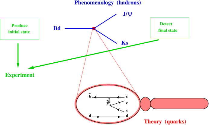
Figure 1: Generic $B$ physics experiment.

One produces the initial state; it time-evolves; eventually it decays; and the final state products are identified in the detector. The experimental details involved in the production of $B$ mesons and in the detection of the final state products have taken thousands of dedicated experimentalists years to perfect and cannot possibly be discussed in these lectures. However, one should be aware that therein lie a number of aspects that even theorists must cope with sooner or later: Which final state particles are easy/difficult to detect?; How do vertexing limitations affect our ability to follow the time-dependent evolution of the initial neutral $B_{d}$ or $B_{s}$ meson?; If we produce initially a $B_{d}-\overline{B_{d}}$ pair, how are these two neutral mesons correlated?; How can that correlation be used to tag the “initial” flavor of the $B_{d}$ meson under study?; and many, many others issues … Here, we will concentrate on the time-evolution and on the decay.

Unfortunately, FIG. 1 already indicates the most serious problem affecting our interpretation of these experiments: the theory is written in terms of the fundamental quark fields; while the experiment deals with hadrons. Indeed, we will need to calculate the matrix elements of the effective quark-field operators when placed in between initial and final states containing hadrons; the so-called hadronic matrix elements:

$$\langle\ \mbox{\small final state hadrons}\ |\ {\cal O}(\mbox{\small quark field operator})\ |\ \mbox{\small initial state hadrons}\ \rangle$$ (5)

Because knowing how the quarks combine into hadrons involves QCD at low energies, these quantities are plagued with uncertainties and are sometimes known as the hadronic “messy” elements.

This is not to say that all is hopeless. Fortunately, on the one hand, there are a number of techniques which allow us to have some control over these quantities in certain special cases and, on the other hand, there are certain decays which have particularly simple interpretations in terms of the parameters in the fundamental weak Lagrangian involving quarks. But this crucial difficulty means that not all experiments have clean theoretical interpretations and forces us to seek information in as many different decays as possible.

One final technical detail is worth mentioning. As emphasized before, the kets corresponding to physical states are defined up to an overall phase [16]; we are free to rephase those kets at will. Of course, any phenomenological parameter describing CP violation must be rephasing invariant and, thus, must arise from the clash of two phases. We will come back to this point in subsection 4.1.1. We are also free to rephase the quark field operators which appear in our theoretical Lagrangian. Again, this implies that all CP violating quantities must arise from the clash of two phases and that we must search for rephasing invariant combinations of the parameters in the weak Lagrangian. This is covered in section 5.3. These two types of rephasing invariance have one further consequence. Many authors write their expressions using specific phase conventions: sometimes these choices are made explicit; sometimes they are not. As a result, we must exercise great care when comparing expressions in different articles and books. Expressions where these questions become acutely critical will be pointed out throughout these lectures.

3 Phenomenology of neutral meson mixing

3.1 Neutral meson mixing: the flavor basis

We are interested in describing the mixing of a neutral meson $P^{0}$ with its antiparticle $\overline{P^{0}}$, where $P$ stands for $K$, $D$, $B_{d}$ or $B_{s}$. We will follow closely the presentation in [23]. In a given approximation [24], we may study the mixing in this particle–antiparticle system separately from its subsequent decay. The time evolution of the state $|\psi(t)\rangle$ describing the $P^{0}-\overline{P^{0}}$ mixed state is given by

$$i\frac{d}{dt}|\psi(t)\rangle=\mbox{\boldmath$H$}\,|\psi(t)\rangle,$$ (6)

where $H$ is a $2\times 2$ matrix written in the $P^{0}-\overline{P^{0}}$ rest frame, and $t$ is the proper time. It is common to break $H$ into its hermitian and anti-hermitian parts, $\mbox{\boldmath$H$}=\mbox{\boldmath$M$}-i/2\mbox{\boldmath$\Gamma$}$, where

$$M = \left(\mbox{\boldmath$H$}+\mbox{\boldmath$H$}^{\dagger}\right)/2,$$

$$-i\mbox{\boldmath$\Gamma$}/2 = \left(\mbox{\boldmath$H$}-\mbox{\boldmath$H$}^{\dagger}\right)/2,$$ (7)

respectively. Both $M$ and $\Gamma$ are hermitian.

The $\{|P^{0}\rangle,|\overline{P^{0}}\rangle\}$ flavor basis satisfies a number of common relations, among which: the orthonormality conditions

$$\langle P^{0}|\overline{P^{0}}\rangle=\langle\overline{P^{0}}|P^{0}\rangle = 0,$$

$$\langle P^{0}|P^{0}\rangle=\langle\overline{P^{0}}|\overline{P^{0}}\rangle = 1;$$ (8)

the fact that $|P^{0}\rangle\langle P^{0}|$ and $|\overline{P^{0}}\rangle\langle\overline{P^{0}}|$ are projection operators; the completeness relation

$$|P^{0}\rangle\langle P^{0}|+|\overline{P^{0}}\rangle\langle\overline{P^{0}}|=1;$$ (9)

and the decomposition of the effective Hamiltonian as

$${\cal H} = |P^{0}\rangle H_{11}\langle P^{0}|+|P^{0}\rangle H_{12}\langle\overline{P^{0}}|+|\overline{P^{0}}\rangle H_{21}\langle P^{0}|+|\overline{P^{0}}\rangle H_{22}\langle\overline{P^{0}}|$$ (13)

$$= \left(\begin{array}[]{cc}|P^{0}\rangle,&|\overline{P^{0}}\rangle\end{array}\right)\mbox{\boldmath$H$}\left(\begin{array}[]{c}\langle P^{0}|\\ \langle\overline{P^{0}}|\end{array}\right).$$

All these relations involve the basis of flavor eigenkets $\{|P^{0}\rangle,|\overline{P^{0}}\rangle\}$ and the basis of the corresponding bras $\{\langle P^{0}|,\langle\overline{P^{0}}|\}$.

Under a CP transformation

$$H_{12}\equiv\langle P^{0}|{\cal H}|\overline{P^{0}}\rangle \stackrel{{\scriptstyle{\cal CP}}}{{\longrightarrow}} \langle P^{0}|({\cal CP})^{\dagger}\ ({\cal CP})\,{\cal H}\,({\cal CP})^{\dagger}\ ({\cal CP})|\overline{P^{0}}\rangle$$ (14)

$$= \langle\overline{P^{0}}|e^{-i\xi}\,{\cal H}_{\rm cp}\,e^{-i\xi}|P^{0}\rangle$$

$$= e^{-2i\xi}\ \langle\overline{P^{0}}|{\cal H}_{\rm cp}|P^{0}\rangle$$

$$H_{11}\equiv\langle P^{0}|{\cal H}|P^{0}\rangle \stackrel{{\scriptstyle{\cal CP}}}{{\longrightarrow}} \langle P^{0}|({\cal CP})^{\dagger}\ ({\cal CP})\,{\cal H}\,({\cal CP})^{\dagger}\ ({\cal CP})|P^{0}\rangle$$ (15)

$$= \langle\overline{P^{0}}|{\cal H}_{\rm cp}|\overline{P^{0}}\rangle,$$

where

$${\cal H}_{\rm cp}\equiv({\cal CP})\,{\cal H}\,({\cal CP})^{\dagger}.$$ (16)

Therefore, if CP is conserved, ${\cal H}={\cal H}_{\rm cp}$,

$$H_{12}=e^{-2i\xi}H_{21}\ \ \ \mbox{and}\ \ \ H_{11}=H_{22}.$$ (17)

Because $\xi$ is a spurious phase without physical significance, we conclude that the phases of $H_{12}$ and $H_{21}$ also lack meaning. (This is clearly understood by noting that these matrix elements change their phase under independent rephasings of $|P^{0}\rangle$ and $|\overline{P^{0}}\rangle$.) As a result, the conclusion with physical significance contained in the first implication of CP conservation in Eq. (17) is $|H_{12}|=|H_{21}|$. A similar study can be made for the other discrete symmetries [1], leading to:

$${\cal CPT}\ \mbox{conservation} \Rightarrow H_{11}=H_{22},$$

$${\cal T}\ \mbox{conservation} \Rightarrow |H_{12}|=|H_{21}|,$$

$${\cal CP}\ \mbox{conservation} \Rightarrow H_{11}=H_{22}\ \mbox{and}\ |H_{12}|=|H_{21}|.$$ (18)

In the most general case, these symmetries are broken and the matrix $H$ is completely arbitrary.

In the rest of this main text we will assume that CPT is conserved and $H_{11}=H_{22}$. As a result, all CP violating observables occurring in $P^{0}-\overline{P^{0}}$ mixing must be proportional to

$$\delta\equiv\frac{|H_{12}|-|H_{21}|}{|H_{12}|+|H_{21}|}.$$ (19)

For completeness, the general case is discussed in appendix A.

3.2 Neutral meson mixing: the mass basis

The time evolution in Eq. (6) becomes trivial in the mass basis which diagonalizes the Hamiltonian $H$. We denote the (complex) eigenvalues of $H$ by

$$\mu_{H} = m_{H}-i/2\Gamma_{H},$$

$$\mu_{L} = m_{L}-i/2\Gamma_{L},$$ (20)

corresponding to the eigenvectors

$$\left(\begin{array}[]{c}|P_{H}\rangle\\ |P_{L}\rangle\end{array}\right)=\left(\begin{array}[]{cc}p&-q\\ p&q\end{array}\right)\ \left(\begin{array}[]{c}|P^{0}\rangle\\ |\overline{P^{0}}\rangle\end{array}\right)=\mbox{\boldmath$X$}^{T}\ \left(\begin{array}[]{c}|P^{0}\rangle\\ |\overline{P^{0}}\rangle\end{array}\right).$$ (29)

Although not strictly necessary, the labels $H$ and $L$ used here stand for the “heavy” and “light” eigenstates respectively. This means that we are using a convention in which $\Delta m=m_{H}-m_{L}>0$. We should also be careful with the explicit choice of $-q$ ($+q$) in the first (second) line of Eq. (29); the opposite choice has been made in references [1, 23]. Remember: in the end, minus signs do matter!!

It is convenient to define

$$m-i\Gamma/2\equiv\mu \equiv \frac{\mu_{H}+\mu_{L}}{2}$$ (30)

$$\Delta m-i\Delta\Gamma/2\equiv\Delta\mu \equiv \mu_{H}-\mu_{L}$$ (31)

The relation between these parameters and the matrix elements of $H$ written in the flavor basis is obtained through the diagonalization

$$\mbox{\boldmath$X$}^{-1}\mbox{\boldmath$H$}\mbox{\boldmath$X$}=\left(\begin{array}[]{cc}\mu_{H}&0\\ 0&\mu_{L}\end{array}\right),$$ (32)

where (Ex-2)

$$\mbox{\boldmath$X$}^{-1}=\frac{1}{2pq}\left(\begin{array}[]{cc}q&-p\\ q&p\end{array}\right).$$ (33)

We find

$$\mu = H_{11}=H_{22},$$ (34)

$$\Delta\mu = 2\sqrt{H_{12}H_{21}},$$ (35)

$$\frac{q}{p} = -\sqrt{\frac{H_{21}}{H_{12}}}=-\frac{2\,H_{21}}{\Delta\mu}.$$ (36)

It is easier to obtain these equations by inverting Eq. (32) (Ex-3):

$$\mbox{\boldmath$H$}=\mbox{\boldmath$X$}\left(\begin{array}[]{cc}\mu_{H}&0\\[5.69054pt] 0&\mu_{L}\end{array}\right)\mbox{\boldmath$X$}^{-1}=\left(\begin{array}[]{cc}\mu&-\frac{\Delta\mu}{2}\frac{p}{q}\\[5.69054pt] -\frac{\Delta\mu}{2}\frac{q}{p}&\mu\end{array}\right).$$ (37)

Eq. (37) is interesting because it expresses the quantities which are calculated in a given theory, $H_{ij}$, in terms of the physical observables. Recall that the phase of $H_{12}$ and, thus, of $q/p$, is unphysical, because it can be changed through independent rephasings of $|P^{0}\rangle$ and $|\overline{P^{0}}\rangle$.

Eq. (35) can be cast in a more familiar form by squaring it and separating the real and imaginary parts, to obtain

$$(\Delta m)^{2}-\frac{1}{4}(\Delta\Gamma)^{2} = 4|M_{12}|^{2}-|\Gamma_{12}|^{2},$$

$$(\Delta m)(\Delta\Gamma) = 4\mbox{Re}(M_{12}^{\ast}\Gamma_{12}).$$ (38)

On the other hand, it is easy to show that

$$\delta=\frac{\left|\frac{p}{q}\right|-\left|\frac{q}{p}\right|}{\left|\frac{p}{q}\right|+\left|\frac{q}{p}\right|}=\frac{2\mbox{Im}(M_{12}^{\ast}\Gamma_{12})}{(\Delta m)^{2}+|\Gamma_{12}|^{2}}.$$ (39)

Eqs. (3.2)–(39) can be rearranged as in (Ex-4).

3.2.1 Mixing in the neutral kaon sector

By accident, the neutral kaon sector satisfies $\Delta m_{K}\approx-\frac{1}{2}\Delta\Gamma_{K}$. On the other hand, $\delta_{K}$ is of order $10^{-3}$. Combining these informations leads to

$$\Delta m\approx 2|M_{12}|\approx-\frac{1}{2}\Delta\Gamma\approx|\Gamma_{12}|,$$ (40)

and, thus,

$$\delta_{K}\approx\frac{\mbox{Im}(M_{12}^{\ast}\ \Gamma_{12}/|\Gamma_{12}|)}{\Delta m}\approx\frac{1}{4}\mbox{Im}\left(\frac{\Gamma_{12}}{M_{12}}\right).$$ (41)

Some authors describe this as the imaginary part of $M_{12}$ because they use a specific phase convention under which $\Gamma_{12}$ is real.

3.2.2 Mixing in the neutral $B_{d}$ and $B_{s}$ systems

In both the $B_{d}$ and $B_{s}$ systems, it can be argued (as we will see below) that $|\Gamma_{12}|\ll|M_{12}|$. As a result,

$$\Delta m_{B} = 2|M_{12}|,$$

$$\Delta\Gamma_{B} = 2\mbox{Re}(M_{12}^{\ast}\Gamma_{12})/|M_{12}|,$$

$$\frac{q}{p} = -\frac{M_{12}^{\ast}}{|M_{12}|}\left[1-\frac{1}{2}\mbox{Im}\left(\frac{\Gamma_{12}}{M_{12}}\right)\right],$$ (42)

where the last expression has been expanded to next-to-leading order in $|\Gamma_{12}/M_{12}|$ [11], so that both the first and last equality in Eq. (39) lead consistently to

$$\delta_{B}\approx\frac{1}{2}\mbox{Im}\left(\frac{\Gamma_{12}}{M_{12}}\right).$$ (43)

We now turn to an intuitive explanation of why $|\Gamma_{12}|$ should be much smaller than $|M_{12}|$ [9, 11]. The idea is the following: one starts from

$$\left|\frac{\Gamma_{12}}{M_{12}}\right|=2\frac{|\Gamma_{12}|/\Gamma}{\Delta m/\Gamma};$$ (44)

one argues that

$$\Gamma_{12}=\sum_{f}\langle f|T|P^{0}\rangle^{\ast}\langle f|T|\overline{P^{0}}\rangle$$ (45)

should be dominated by the Standard Model tree-level diagrams; one estimates what this contribution might be; and, finally, one uses a measurement of $x_{d}=(\Delta m/\Gamma)_{B_{d}}=0.771\pm 0.012$ and an upper bound on $x_{s}=(\Delta m/\Gamma)_{B_{s}}>20.6$ with C.L.$=95\%$ from experiment [17].

Clearly, Eq. (45) only involves channels common to $P^{0}$ and $\overline{P^{0}}$. In the $B_{d}$ system, such channels are CKM-suppressed and their branching ratios are at or below the level of $10^{-3}$. Moreover, they come into Eq. (45) with opposite signs. Therefore, one expects that the sum does not exceed the individual level, leading to $|\Gamma_{12}|/\Gamma<10^{-2}$ as a rather safe bound. Combined with $x_{d}$, we obtain $|\delta_{B_{d}}|<{\cal O}\left(10^{-2}\right)$ for the $B_{d}$ system.

The situation in the $B_{s}$ system is rather different because the dominant decays common to $B^{0}_{s}$ and $\overline{B^{0}_{s}}$ are due to the tree-level transitions $b\rightarrow c\bar{c}s$. Therefore, $\Gamma_{12}/\Gamma$ is expected to be large. One estimate by Beneke, Buchalla and Dunietz yields [26],

$$\left|\frac{\Gamma_{12}}{\Gamma}\right|=\frac{1}{2}\left(0.16^{+0.11}_{-0.09}\right).$$ (46)

Fortunately, this large value is offset by the strong lower bound on $x_{s}$, leading, again, to $|\delta_{B_{s}}|<{\cal O}\left(10^{-2}\right)$.

These arguments are rather general and should hold in a variety of new physics models. Precise calculations within the SM lead to $\delta_{B_{d}}\sim-2.5\times 10^{-4}$ and $\delta_{B_{s}}\sim 0.1\times 10^{-4}$ [25].

Incidentally, the analysis discussed here means that $\Delta\Gamma$ can be set to zero in the $B_{d}$ system but that it must be taken into account in the time evolution of the $B_{s}$ system [27].

3.3 The need for the reciprocal basis

We now come to a problem frequently overlooked. Is the matrix $X$ in Eq. (32) a unitary matrix or not? The answer comes from introductory algebra: matrices satisfying $[\mbox{\boldmath$H$},\mbox{\boldmath$H$}^{\dagger}]=0$ are called “normal” matrices. Equivalent definitions are (that is to say that $H$ is normal if and only if): i) $X$ is a unitary matrix; ii) the left-eingenvectors and the right-eigenvectors of $H$ coincide; iii) $[\mbox{\boldmath$M$},\mbox{\boldmath$\Gamma$}]=0$; among many other possible equivalent statements.

Now, the 1964 experiment mentioned above implies that $|H_{12}|\neq|H_{21}|$ holds in the neutral kaon system, thus establishing CP and T violation in the $K^{0}-\overline{K^{0}}$ mixing. But, this also has an important implication for the matrix $X$. Indeed, the $(1,1)$ entry in the matrix $[\mbox{\boldmath$H$},\mbox{\boldmath$H$}^{\dagger}]$ is given by $|H_{12}|^{2}-|H_{21}|^{2}$. Therefore, that experimental result also implies that the matrix $H$ is not normal and, thus, that we are forced to deal with non-unitary matrices in the neutral kaon system (Ex-5). As for the other neutral meson systems, $|H_{12}|\neq|H_{21}|$ has not yet been established experimentally. Nevertheless, the Standard Model predicts that, albeit the difference is small, $|H_{12}|\neq|H_{21}|$ does indeed hold. As before, this implies CP violation in the mixing and forces the use of a non-unitary mixing matrix $X$ [23].

So, why do (most) people worry about performing non-unitary transformations? The reason is that one would like the mass basis $\{|P_{H}\rangle,|P_{L}\rangle\}$ to retain a number of the nice (orthonormality) features of the $\{|P^{0}\rangle,|\overline{P^{0}}\rangle\}$ flavor basis; Eqs. (8)–(13). The problem is that, when $H$ is not normal, we cannot find similar relations involving the basis of mass eigenkets $\left\{|P_{H}\rangle,|P_{L}\rangle\right\}$ and the basis of the corresponding bras, $\left\{\langle P_{H}|,\langle P_{L}|\right\}$. Indeed, substituting Eq. (37) into Eq. (13) we find

$${\cal H} = \left(\begin{array}[]{cc}|P^{0}\rangle,&|\overline{P^{0}}\rangle\end{array}\right)\,\mbox{\boldmath$X$}\left(\begin{array}[]{cc}\mu_{H}&0\\[5.69054pt] 0&\mu_{L}\end{array}\right)\mbox{\boldmath$X$}^{-1}\,\left(\begin{array}[]{c}\langle P^{0}|\\ \langle\overline{P^{0}}|\end{array}\right)$$ (52)

$$= \left(\begin{array}[]{cc}|P_{H}\rangle,&|P_{L}\rangle\end{array}\right)\left(\begin{array}[]{cc}\mu_{H}&0\\ 0&\mu_{L}\end{array}\right)\left(\begin{array}[]{c}\langle\tilde{P}_{H}|\\ \langle\tilde{P}_{L}|\end{array}\right)$$ (58)

$$= |P_{H}\rangle\mu_{H}\langle\tilde{P}_{H}|+|P_{L}\rangle\mu_{L}\langle\tilde{P}_{L}|$$ (59)

This does not involve the bras $\langle P_{H}|$ and $\langle P_{L}|$,

$$\left(\begin{array}[]{c}\langle P_{H}|\\ \langle P_{L}|\end{array}\right)=\mbox{\boldmath$X$}^{\dagger}\left(\begin{array}[]{c}\langle P^{0}|\\ \langle\overline{P^{0}}|\end{array}\right),$$ (60)

but rather the so called ‘reciprocal basis’

$$\left(\begin{array}[]{c}\langle\tilde{P}_{H}|\\ \langle\tilde{P}_{L}|\end{array}\right)=\mbox{\boldmath$X$}^{-1}\left(\begin{array}[]{c}\langle P^{0}|\\ \langle\overline{P^{0}}|\end{array}\right).$$ (61)

The reciprocal basis may also be defined by the orthonormality conditions

$$\langle\tilde{P}_{H}|P_{L}\rangle=\langle\tilde{P}_{L}|P_{H}\rangle = 0,$$

$$\langle\tilde{P}_{H}|P_{H}\rangle=\langle\tilde{P}_{L}|P_{L}\rangle = 1.$$ (62)

Moreover, $|P_{H}\rangle\langle\tilde{P}_{H}|$ and $|P_{L}\rangle\langle\tilde{P}_{L}|$ are projection operators, and the partition of unity becomes

$$|P_{H}\rangle\langle\tilde{P}_{H}|+|P_{L}\rangle\langle\tilde{P}_{L}|=1.$$ (63)

If $H$ is not normal, then $X$ is not unitary, and $\left\{\langle P_{H}|,\langle P_{L}|\right\}$ in Eq. (60) do not coincide with $\left\{\langle\tilde{P}_{H}|,\langle\tilde{P}_{L}|\right\}$ in Eq. (61). Another way to state this fact is to note that $H$ is normal ($X$ is unitary) if and only if its right-eigenvectors coincide with its left-eigenvectors.

That these features have an impact on the $K^{0}-\overline{K^{0}}$ system, was pointed out long ago by Sachs [28, 29], by Enz and Lewis [30], and by Wolfenstein [31]. More recently, they have been stressed by Beuthe, López-Castro and Pestieu [32], by Alvarez-Gaumé et al. [33], by Branco, Lavoura and Silva in their book “CP violation” [1], and expanded by Silva in [23].

We stress that this is not a side issue. For example, if we wish to describe a final state containing a $K_{S}$, as we will do when discussing the extremely important $B_{d}\rightarrow J/\psi K_{S}$ decay, we will need to know that the correct “bra” to describe a $K_{S}$ in the final state is $\langle\tilde{K}_{S}|$, and not $\langle K_{S}|$.

3.4 Time evolution

As mentioned, the time evolution is trivial in the mass basis:

$$|P_{H}(t)\rangle = e^{-i\mu_{H}\,t}|P_{H}\rangle\ ,$$

$$|P_{L}(t)\rangle = e^{-i\mu_{L}\,t}|P_{L}\rangle\ .$$ (64)

This can be used to study the time evolution in the flavor basis. Let us suppose that we have identified a state as $P^{0}$ at time $t=0$. Inverting Eq. (29), we may write the initial state as

$$|P^{0}\rangle=\frac{1}{2\,p}\left(|P_{H}\rangle+|P_{L}\rangle\right).$$ (65)

From Eq. (64) we know that, at a later time $t$, this state will have evolved into

$$|P^{0}(t)\rangle=\frac{1}{2\,p}\left(e^{-i\mu_{H}\,t}|P_{H}\rangle+e^{-i\mu_{L}\,t}|P_{L}\rangle\right),$$ (66)

which, using again Eq. (29), may be rewritten in the flavor basis as

$$|P^{0}(t)\rangle=\frac{1}{2}\left(e^{-i\mu_{H}\,t}+e^{-i\mu_{L}\,t}\right)|P^{0}\rangle-\frac{q}{p}\,\frac{1}{2}\left(e^{-i\mu_{H}\,t}-e^{-i\mu_{L}\,t}\right)|\overline{P^{0}}\rangle.$$ (67)

It is easy to repeat this exercise in order to describe the time evolution $|\overline{P^{0}}(t)\rangle$ of a state identified as $\overline{P^{0}}$ at time $t=0$. Introducing the auxiliary functions

$$g_{\pm}(t)\equiv\pm\frac{1}{2}\left(e^{-i\mu_{H}\,t}\pm e^{-i\mu_{L}\,t}\right)=e^{-im\,t}\ e^{-\Gamma\,t/2}\left\{\begin{array}[]{l}\cos{\left(\frac{\Delta\mu t}{2}\right)}\\ i\sin{\left(\frac{\Delta\mu t}{2}\right)}\end{array}\right..$$ (68)

we can combine both results into

$$|P^{0}(t)\rangle = g_{+}(t)|P^{0}\rangle+\frac{q}{p}g_{-}(t)|\overline{P^{0}}\rangle\ ,$$

$$|\overline{P^{0}}(t)\rangle = \frac{p}{q}g_{-}(t)|P^{0}\rangle+g_{+}(t)|\overline{P^{0}}\rangle\ ,$$ (69)

These results may also be obtained making full use of the matrix notation introduced in the preceding sections (Ex-6).

Eq. (68) contains another expression for which there are many choices in the literature. The explicit $-$ sign we have chosen here for the definition of $g_{-}(t)$ is not universal. For instances, the $+$ sign has been chosen for the definition of $g_{-}(t)$ in references [1, 23]. This goes unnoticed in all expressions involving the product of $q$ and $g_{-}(t)$, because the minus signs introduced in both definitions cancel. This is also the notation used in the recent PDG review by Schneider on $B^{0}-\overline{B^{0}}$ mixing. Another notation is used in the recent PDG review of CP violation by Kirby and Nir [17]; they use the sign of $q$ in Eq. (29), but define $g_{-}(t)$ without the explicit minus sign in Eq. (68). I cannot stress this enough: when comparing different articles you should check all definitions first.

4 Phenomenology of the production and decay of neutral mesons

4.1 Identifying the relevant parameters

Let us consider the chain $i\rightarrow P+X\rightarrow f+X$ shown in FIG. 2,

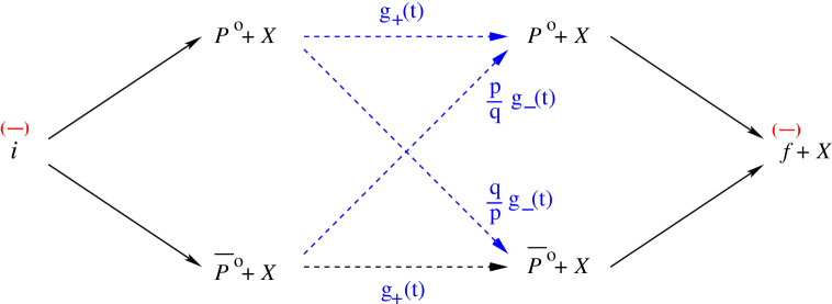
Figure 2: Schematic description of the decay chain $i\rightarrow P+X\rightarrow f+X$.

in which the initial state $i$ originates the production of a neutral meson $P$, which evolves in time, decaying later into a final state $f$. In what follows we will skip the explicit reference to the set of particles $X$ which is produced in association with the neutral meson $P$, except in appendix B, where the explicit reference to $X$ will become necessary.

The amplitude for this decay chain (and its CP conjugated) depends on the amplitudes for the initial process

$$A_{i\rightarrow P^{0}}\equiv\langle P^{0}|T|i\rangle\ , A_{\bar{i}\rightarrow P^{0}}\equiv\langle P^{0}|T|\bar{i}\rangle\ ,$$

$$A_{i\rightarrow\overline{P^{0}}}\equiv\langle\overline{P^{0}}|T|i\rangle\ , A_{\bar{i}\rightarrow\overline{P^{0}}}\equiv\langle\overline{P^{0}}|T|\bar{i}\rangle\ ;$$ (70)

it depends on the parameters describing the time-evolution of the neutral $P$ system, including $q/p$; and it also depends on the amplitudes for the decay into the final state,

$$A_{f}\equiv\langle f|T|P^{0}\rangle\ , A_{\bar{f}}\equiv\langle\bar{f}|T|P^{0}\rangle\ ,$$

$$\bar{A}_{f}\equiv\langle f|T|\overline{P^{0}}\rangle\ , \bar{A}_{\bar{f}}\equiv\langle\bar{f}|T|\overline{P^{0}}\rangle\ .$$ (71)

As mentioned, all states may be redefined by an arbitrary phase transformation [16]. Such transformations change the mixing parameters and the transition amplitudes. Clearly, the magnitudes of the transition amplitudes and the magnitude $|q/p|$ are all invariant under those transformations. Besides these magnitudes, there are quantities which are invariant under those arbitrary phase redefinitions and which arise from the “interference” between the parameters describing the mixing and the parameters describing the transitions:

$$\lambda_{f}\equiv\frac{q}{p}\frac{\bar{A}_{f}}{A_{f}}\ , \lambda_{\bar{f}}\equiv\frac{q}{p}\frac{\bar{A}_{\bar{f}}}{A_{\bar{f}}}\ ,$$ (72)

$$\xi_{i\rightarrow P}\equiv\frac{A_{i\rightarrow\overline{P^{0}}}}{A_{i\rightarrow P^{0}}}\frac{p}{q}\ , \xi_{\bar{i}\rightarrow P}\equiv\frac{A_{\bar{i}\rightarrow\overline{P^{0}}}}{A_{\bar{i}\rightarrow P^{0}}}\frac{p}{q}\ .$$ (73)

The parameters in Eq. (72) describe the interference between the mixing in the $P^{0}-\overline{P^{0}}$ system and the subsequent decay from that system into the final states $f$ and $\bar{f}$, respectively. In contrast, the parameters in Eq. (73) describe the interference between the production of the system $P^{0}-\overline{P^{0}}$ and the mixture in that system.

4.1.1 The usual three types of CP violation

With a simple analysis described in appendix B, we can identify those observables which signal CP violation:

1. $|q/p|-1$ describes CP violation in the mixing of the neutral meson system;

2. $|A_{i\rightarrow P^{0}}|-|A_{\bar{i}\rightarrow\overline{P^{0}}}|$ and $|A_{i\rightarrow\overline{P^{0}}}|-|A_{\bar{i}\rightarrow P^{0}}|$, on the one hand, and $|A_{f}|-|\bar{A}_{\bar{f}}|$ and $|A_{\bar{f}}|-|\bar{A}_{f}|$, on the other hand, describe the CP violation present directly in the production of the neutral meson system and in its decay, respectively;

3. $\arg\lambda_{f}+\arg\lambda_{\bar{f}}$ measures the CP violation arising from the interference between mixing in the neutral meson system and its subsequent decay into the final states $f$ and $\bar{f}$. We call this the “interference CP violation: first mix, then decay”. When $f=f_{cp}$ is an CP eigenstate, this CP violating observable $\arg\lambda_{f}+\arg\lambda_{\bar{f}}$, becomes proportional to $\mbox{Im}\lambda_{f}$.

These are the types of CP violation discussed in the usual presentations of CP violation, since they are the ones involved in the evolution and decay of the neutral meson system (cf. section 4.2).

These three types of CP violation have been measured. And, due to the rephasing freedom $|P^{0}\rangle\rightarrow e^{i\gamma}|P^{0}\rangle$, these must arise from the clash between two phases. More information about these types of CP violation will be discussed in later sections. The combination of all this information may be summarized schematically as:

1. Clash mixing $M_{12}$ with $\Gamma_{12}$: $|q/p|-1$

   • CPV in mixing

   • measured in kaon system through $\epsilon_{K}$

   

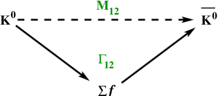
   Figure 3: Schematic mixing CP violation in neutral kaon mixing.

2. Clash two direct decay paths: $|\bar{A}/A|-1$

   • CPV in decay

   • measured in kaon system through $\epsilon^{\prime}_{K}$

   

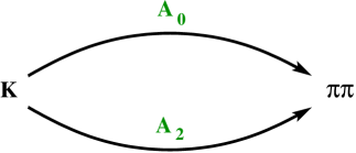
   Figure 4: Schematic direct CP violation in neutral kaon decays into two pions.

3. Clash direct path with mixing path; first mix–then decay: $\lambda_{f}=q_{B}/p_{B}\ \bar{A}_{f}/A_{f}$

   • CPV in interference; first mix–then decay

   • measured in $B_{d}$ system through $\sin{2\beta}$

   

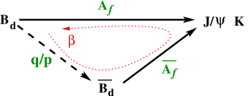
   Figure 5: Schematic interference CP violation in the decay $B_{d}\rightarrow J/\psi K_{S}$.

4.1.2 A fourth type of CP violation

However, in considering the production mechanism of the neutral meson system we are lead to consider a novel observable, which also signals CP violation,

$$\arg\xi_{i\rightarrow P}+\arg\xi_{\bar{i}\rightarrow P}.$$ (74)

This observable measures the CP violation arising from the interference between the production of the neutral meson system and the mixing in that system. We call this the “interference CP violation: first produce, then mix”. This was first identified in 1998 by Meca and Silva [36], when studying the effect of $D^{0}-\overline{D^{0}}$ mixing on the decay chain

$$B^{\pm}\rightarrow\{D^{0},\overline{D^{0}}\}K^{\pm}\rightarrow[f]_{D}K^{\pm}.$$ (75)

Later, Amorim, Santos and Silva showed that adding these new parameters $\xi_{i\rightarrow P}$ and $\xi_{\bar{i}\rightarrow P}$ is enough to describe fully any decay chain involving a neutral meson system as an intermediate step [34].

This information may be summarized schematically as:

• Clash direct path with mixing path; first produce–then decay: $\xi_{i}=A_{i\rightarrow D}/A_{i\rightarrow\bar{D}}\ p_{D}/q_{D}$

  • CPV in interference; first mix–then decay

  • Never measured

  • It can affect the determination of $\gamma$ from $B\rightarrow D$ decays

  

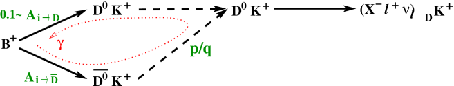
  Figure 6: Schematic interference CP violation in the decay chain $B^{+}\rightarrow DK^{+}\rightarrow D^{0}K^{+}$.

It is easy to see from the decay chain in FIG. 6 that none of the types of CP violation described in the previous subsection is involved here: because we are using a charged $B$ meson, we are not sensitive to the mixing or interference CP violation involved in the decays of neutral $B$ mesons; there is also no direct CP violation in $B\rightarrow D$ decays. Furthermore, this effect is present already within the Standard Model, and it involves the weak phase $\gamma$ to be discussed later.

Of course, a non-zero mixing in the $D^{0}-\overline{D^{0}}$ system is required. A mixing of order $10^{-2}$ is still allowed by experiment, which competes against $A_{i\rightarrow D}/A_{i\rightarrow\bar{D}}\sim 10^{-1}$. Therefore, the lower decay path may give a correction of order $10\%$ to the upper decay path. It would be very interesting to measure this new type of CP violation, specially because it flies in the face of popular wisdom. In any case, this effect has to be taken into account as a source of systematic uncertainty in the extraction of $\gamma$ from $B\rightarrow D$ decays, such as $B^{\pm}\rightarrow DK^{\pm}$ [37].

4.2 Decays from a neutral meson system

Henceforth, we will ignore the production mechanism and concentrate on the time-dependent decay rates from a neutral meson system into a final state $f$. These formulae are used in the description of the CP violating asymmetries in section 4.4.

Let us consider the decay of a state $P^{0}$ or $\overline{P^{0}}$ into the final state $f$. These decays depend on two decay amplitudes

$$A_{f} \equiv \langle f|T|P^{0}\rangle,$$

$$\bar{A}_{f} \equiv \langle f|T|\overline{P^{0}}\rangle.$$ (76)

A state identified as the eigenvector of the strong interaction (flavor eigenstate) $P^{0}$ at time $t=0$, will evolve in time according to Eq. (69) and, thus, decay into the final state $f$ at time $t$ with an amplitude

$$A\left[P^{0}(t)\rightarrow f\right]=\langle f|T|P^{0}(t)\rangle=g_{+}(t)A_{f}+\frac{q}{p}g_{-}(t)\bar{A}_{f}.$$ (77)

Similarly, the decay amplitude for a state identified at time $t=0$ as $\overline{P^{0}}$ is given by

$$A\left[\overline{P^{0}}(t)\rightarrow f\right]=\langle f|T|\overline{P^{0}}(t)\rangle=\frac{p}{q}g_{-}(t)A_{f}+g_{+}(t)\bar{A}_{f}.$$ (78)

The corresponding decay probabilities into the CP conjugated states $f$ and $\bar{f}$ are given by

$$\Gamma[P^{0}(t)\rightarrow f] = \left|A_{f}\right|^{2}\left\{\left|g_{+}(t)\right|^{2}+\left|\lambda_{f}\right|^{2}\left|g_{-}(t)\right|^{2}+2\mbox{Re}\left[\lambda_{f}g_{+}^{\ast}(t)g_{-}(t)\right]\right\}$$

$$\Gamma[P^{0}(t)\rightarrow\bar{f}] = \left|\bar{A}_{\bar{f}}\right|^{2}\left|\frac{q}{p}\right|^{2}\left\{\left|g_{-}(t)\right|^{2}+\left|\bar{\lambda}_{\bar{f}}\right|^{2}\left|g_{+}(t)\right|^{2}+2\mbox{Re}\left[\bar{\lambda}_{\bar{f}}\,g_{+}(t)g_{-}^{\ast}(t)\right]\right\},$$

$$\Gamma[\overline{P^{0}}(t)\rightarrow f] = \left|A_{f}\right|^{2}\left|\frac{p}{q}\right|^{2}\left\{\left|g_{-}(t)\right|^{2}+\left|\lambda_{f}\right|^{2}\left|g_{+}(t)\right|^{2}+2\mbox{Re}\left[\lambda_{f}g_{+}(t)g_{-}^{\ast}(t)\right]\right\},$$

$$\Gamma[\overline{P^{0}}(t)\rightarrow\bar{f}] = \left|\bar{A}_{\bar{f}}\right|^{2}\left\{\left|g_{+}(t)\right|^{2}+\left|\bar{\lambda}_{\bar{f}}\right|^{2}\left|g_{-}(t)\right|^{2}+2\mbox{Re}\left[\bar{\lambda}_{\bar{f}}g_{+}^{\ast}(t)g_{-}(t)\right]\right\},$$ (79)

where we have used the definitions of $\lambda_{f}$ in Eq. (72) and $\bar{\lambda}_{\bar{f}}\equiv 1/\lambda_{\bar{f}}$, while the functions governing the time evolution are given by (Ex-7)

$$|g_{\pm}(t)|^{2} = \frac{1}{4}\left[e^{-\Gamma_{H}t}+e^{-\Gamma_{L}t}\pm 2e^{-\Gamma t}\cos(\Delta m\,t)\right]$$

$$= \frac{e^{-\Gamma t}}{2}\left[\cosh\frac{\Delta\Gamma t}{2}\pm\cos\left(\Delta mt\right)\right],$$

$$g_{+}^{\ast}(t)g_{-}(t) = \frac{1}{4}\left[-e^{-\Gamma_{H}t}+e^{-\Gamma_{L}t}+2ie^{-\Gamma t}\sin(\Delta m\,t)\right]$$ (80)

$$= \frac{e^{-\Gamma t}}{2}\left[\sinh\frac{\Delta\Gamma t}{2}+i\sin\left(\Delta mt\right)\right].$$

Eqs. (79) give us the probability, divided by $dt$, that the state identified as $P^{0}$ (or $\overline{P^{0}}$) decays into the final state $f$ (or $\bar{f}$) during the time-interval $[t,t+dt]$. The time-integrated expressions are identical to these, with the substitution of $|g_{+}(t)|^{2}$, $|g_{-}(t)|^{2}$, and $g_{+}^{\ast}(t)g_{-}(t)$ by (Ex-8)

$$G_{\pm} \equiv \displaystyle\int_{0}^{+\infty}\!|g_{\pm}(t)|^{2}dt=\frac{1}{2\Gamma}\left(\frac{1}{1-y^{2}}\pm\frac{1}{1+x^{2}}\right),$$

$$G_{+-} \equiv \int_{0}^{+\infty}\!g_{+}^{\ast}(t)g_{-}(t)dt=\frac{1}{2\Gamma}\left(\frac{y}{1-y^{2}}+\frac{ix}{1+x^{2}}\right),$$ (81)

where,

$$x\equiv\frac{\Delta m}{\Gamma}\ \ \ \mbox{and}\ \ \ y\equiv\frac{\Delta\Gamma}{2\Gamma}.$$ (82)

4.3 Flavor-specific decays and CP violation in mixing

Let us denote by $o$ a final state to which only $P^{0}$ may decay, and by $\bar{o}$ its CP conjugated state, to which only $\overline{P^{0}}$ can decay. For example, $o$ could be a semileptonic final state such as in

$$K^{0}\rightarrow\pi^{-}l^{+}\nu_{l}\ \ \ \ \ \mbox{or}\ \ \ \ \ B^{0}_{d}\rightarrow h^{-}l^{+}\nu_{l},$$ (83)

where $h^{-}$ is a negatively charged hadron, $l^{+}$ a charged anti-lepton ($e^{+}$, $\mu^{+}$, or $\tau^{+}$), and $\nu_{l}$ the corresponding neutrino. Thus, $A_{\bar{o}}=\langle\bar{o}|T|P^{0}\rangle=0$, $\bar{A}_{o}=\langle o|T|\overline{P^{0}}\rangle=0$, and Eqs. (79) become

$$\Gamma[P^{0}(t)\rightarrow o] = \left|A_{o}\right|^{2}\left|g_{+}(t)\right|^{2}$$

$$\Gamma[P^{0}(t)\rightarrow\bar{o}] = \left|\bar{A}_{\bar{o}}\right|^{2}\left|\frac{q}{p}\right|^{2}\left|g_{-}(t)\right|^{2}$$

$$\Gamma[\overline{P^{0}}(t)\rightarrow o] = \left|A_{o}\right|^{2}\left|\frac{p}{q}\right|^{2}\left|g_{-}(t)\right|^{2}$$

$$\Gamma[\overline{P^{0}}(t)\rightarrow\bar{o}] = \left|\bar{A}_{\bar{o}}\right|^{2}\left|g_{+}(t)\right|^{2}$$ (84)

Clearly, $\Gamma[P^{0}(t)\rightarrow\bar{o}]$ and $\Gamma[\overline{P^{0}}(t)\rightarrow o]$ vanish at $t=0$, but they are non-zero at $t\neq 0$ due to the mixing of the neutral mesons.

We may test for CP violation through the asymmetry (Ex-9)

$$A_{M} = \frac{\Gamma[\overline{P^{0}}(t)\rightarrow o]-\Gamma[P^{0}(t)\rightarrow\bar{o}]}{\Gamma[\overline{P^{0}}(t)\rightarrow o]+\Gamma[P^{0}(t)\rightarrow\bar{o}]}$$ (85)

$$= \frac{\left|p/q\right|^{2}-\left|q/p\right|^{2}}{\left|p/q\right|^{2}+\left|q/p\right|^{2}}=\frac{2\delta}{1+\delta^{2}}$$

$$= \frac{\left|H_{12}\right|^{2}-\left|H_{21}\right|^{2}}{\left|H_{12}\right|^{2}+\left|H_{21}\right|^{2}}=\frac{4\mbox{Im}\left(M_{12}^{\ast}\Gamma_{12}\right)}{4\left|M_{12}\right|^{2}+\left|\Gamma_{12}\right|^{2}},$$

where we have used $|A_{o}|=|\bar{A}_{\bar{o}}|$. Notice that this asymmetry does not depend on $t$. This measures $\delta$, i.e., it probes CP violation in mixing. Because it is usually performed with the semileptonic decays in Eq. (83), this is also known as the semileptonic decay asymmetry $a_{SL}$.

In the kaon system, we can use the approximate experimental equalities in Eq. (40) in order to find

$$A_{M}\approx\frac{1}{2}\mbox{Im}\left(\Gamma_{12}/M_{12}\right),$$ (86)

which, of course, agrees with Eq. (41). In fact CP violation in mixing has been measured in the kaon system both through the $K_{L}\rightarrow\pi\pi$ decays and through the semileptonic decays.

As discussed in subsection 3.2.2, $\delta$ is expected to be very small for the $B_{d}$ and $B_{s}$ systems. Because we will be looking for other CP violating effects of order one, we will neglect mixing CP violation in our ensuing discussion of the $B$ meson systems.

4.4 Approximations and notation for $B$ decays

In the next few years we will gain further information about CP violation from the BABAR and Belle experiments, concerning mainly $B^{\pm}$ and $B_{d}$ decays, conjugated from results from CDF and DØ(and, later, BTeV and LHCb), which also detect $B_{s}$.

We will use the following approximations discussed in subsection 3.2.2:

$$\mbox{both}\ \ B_{d}\ \ \mbox{and}\ \ B_{s}\ \ \mbox{systems} \Longrightarrow \left|\frac{q}{p}\right|=1\ \ \Longrightarrow\ \ |\lambda_{f}|=\left|\frac{\bar{A}_{f}}{A_{f}}\right|,$$ (87)

$$\mbox{only}\ \ B_{d}\ \ \mbox{system} \Longrightarrow \Delta\Gamma=0$$ (88)

The first approximation leads to

$$\frac{q}{p}=-\frac{2\,M_{21}}{\Delta m}=-\frac{M_{12}^{\ast}}{|M_{12}|},$$ (89)

which will later be used to calculate $q/p$ in the Standard Model. However, we know from Eqs. (17) and (36) that CP conservation in the mixing implies that

$$\frac{q}{p}=-\eta_{P}e^{i\xi},$$ (90)

where $\xi$ is the arbitrary CP transformation phase in Eq. (1). The sign $\eta_{P}=\pm 1$ arises from the square root in Eq. (36) and, according to Eq. (29), it leads to ${\cal CP}|P_{H}\rangle=\eta_{P}|P_{H}\rangle$. That is, $\eta_{P}$, defined in the limit of CP conservation in the mixing, is measurable and it determines whether the heavier eigenstate is CP even ($\eta_{P}=1$) or CP odd ($\eta_{P}=-1$), in that limit. (See also appendix B.) Expressions (89) and (90) are often mishandled, a fact we will come back to in section 6.1.

For the $B_{s}$ system, we use the first approximation to transform the time-dependent decay probabilities of Eq. (79) into (Ex-10)

$$\Gamma[B^{0}_{s}(t)\rightarrow f] = \frac{\left|A_{f}\right|^{2}+\left|\bar{A}_{f}\right|^{2}}{2}\ e^{-\Gamma\,t}\,\left\{\cosh{\left(\frac{\Delta\Gamma\,t}{2}\right)}+D_{f}\sinh{\left(\frac{\Delta\Gamma\,t}{2}\right)}\right.$$

$$\hskip 99.58464pt\left.+\;C_{f}\cos{(\Delta m\,t)}-S_{f}\sin{(\Delta m\,t)}\right\},$$

$$\Gamma[\overline{B^{0}_{s}}(t)\rightarrow f] = \frac{\left|A_{f}\right|^{2}+\left|\bar{A}_{f}\right|^{2}}{2}\ e^{-\Gamma\,t}\,\left\{\cosh{\left(\frac{\Delta\Gamma\,t}{2}\right)}+D_{f}\sinh{\left(\frac{\Delta\Gamma\,t}{2}\right)}\right.$$ (91)

$$\hskip 99.58464pt\left.-\;C_{f}\cos{(\Delta m\,t)}+S_{f}\sin{(\Delta m\,t)}\right\},$$

where

$$D_{f} \equiv \frac{2\mbox{Re}(\lambda_{f})}{1+|\lambda_{f}|^{2}}$$ (92)

$$C_{f} \equiv \frac{1-|\lambda_{f}|^{2}}{1+|\lambda_{f}|^{2}}$$ (93)

$$S_{f} \equiv \frac{2\mbox{Im}(\lambda_{f})}{1+|\lambda_{f}|^{2}}.$$ (94)

Clearly (Ex-11),

$$\lambda_{f}=\frac{1}{1+C_{f}}\left(D_{f}+iS_{f}\right)$$ (95)

is a physical observable, and

$$D_{f}^{2}+C_{f}^{2}+S_{f}^{2}=1.$$ (96)

Therefore, $C_{f}^{2}+S_{f}^{2}\leq 1$, with the equality holding if and only if $\lambda_{f}$ is purely imaginary. The importance of $\Delta\Gamma$ on the $B_{s}$ system in order to provide a separate handle on $D_{f}$, and in order to enable the use of untagged decays was first pointed out by Dunietz [27].

The expressions for the $B_{d}$ system are simplified by setting $\Delta\Gamma=0$, to obtain

$$\Gamma[B^{0}_{d}(t)\rightarrow f] = \frac{\left|A_{f}\right|^{2}+\left|\bar{A}_{f}\right|^{2}}{2}\ e^{-\Gamma\,t}\,\left\{1+C_{f}\cos{(\Delta m\,t)}-S_{f}\sin{(\Delta m\,t)}\right\},$$

$$\Gamma[\overline{B^{0}_{d}}(t)\rightarrow f] = \frac{\left|A_{f}\right|^{2}+\left|\bar{A}_{f}\right|^{2}}{2}\ e^{-\Gamma\,t}\,\left\{1-C_{f}\cos{(\Delta m\,t)}+S_{f}\sin{(\Delta m\,t)}\right\}.$$ (97)

Notice that, in this approximation of $\Delta\Gamma=0$, $D_{f}$ is not measured. It can be inferred from Eq. (96) with a twofold ambiguity, meaning that $\lambda_{f}$ is determined from Eq. (95) with that twofold ambiguity. In Eq. (93) we used $C_{f}$ as defined by BABAR. When comparing results, you should note that Belle uses a different notation

$${\cal A}_{f}\left(\mbox{Belle}\right)=-C_{f}\left(\mbox{BABAR}\right).$$ (98)

Here is another place where competing definitions abound in the literature. For example, reference [1] uses $a^{\rm dir}=C_{f}$ and, because of the sign change in the definition of $q$, $a^{\rm int}=-S_{f}$.

In order to test CP, we must compare $B^{0}(t)\rightarrow f$ with $\overline{B^{0}}(t)\rightarrow\bar{f}$, or $B^{0}(t)\rightarrow\bar{f}$ with $\overline{B^{0}}(t)\rightarrow f$. To simplify the discussion we will henceforth concentrate on decays into final states $f_{\rm cp}$ which are CP eigenstates:

$${\cal CP}|f_{\rm cp}\rangle=\eta_{f}|f_{\rm cp}\rangle,$$ (99)

where $\eta_{f}=\pm 1$. For these, we define the CP asymmetry

$$A_{\rm CP}(t) \equiv \frac{\Gamma[\overline{B^{0}}(t)\rightarrow f_{\rm cp}]-\Gamma[B^{0}(t)\rightarrow f_{\rm cp}]}{\Gamma[\overline{B^{0}}(t)\rightarrow f_{\rm cp}]+\Gamma[B^{0}(t)\rightarrow f_{\rm cp}]}$$ (100)

$$= -C_{f}\cos{\Delta mt}+S_{f}\sin{\Delta mt}.$$ (101)

This is another place where two possibilities exist in the literature. Although this seems to be the most common choice nowadays, some authors define $A_{\rm CP}(t)$ to have the opposite sign, specially in their older articles.

Since we have assumed that $|q/p|=1$, $1-|\lambda_{f}|^{2}\propto|A_{f}|^{2}-|\bar{A}_{f}|^{2}$, and $C_{f}$ measures CP violation in the decay amplitudes. On the other had, $S_{f}\propto\mbox{Im}\lambda_{f}$ measures CP violation in the interference between the mixing in the $B^{0}_{d}-\overline{B^{0}_{d}}$ system and its decay into the final state $f_{\rm cp}$.

There is a similar CP violating asymmetry defined for charged $B$ decays. However, since there is no mixing (of course), it only detects direct CP violation

$$A_{D}\equiv\frac{\Gamma[B^{+}\rightarrow f^{+}]-\Gamma[B^{-}\rightarrow f^{-}]}{\Gamma[B^{+}\rightarrow f^{+}]+\Gamma[B^{-}\rightarrow f^{-}]}=\frac{|A_{+}|^{2}-|A_{-}|^{2}}{|A_{+}|^{2}+|A_{-}|^{2}},$$ (102)

where the notation is self-explanatory.

4.5 Checklist of crucial notational signs

There are countless reviews and articles on CP violation, each with its own notational hazards. When reading any given article, there are a few signs whose definition is crucial. We have mentioned them when they arose, and we collect them here for ease of reference. One should check:

1. the sign of $q$ in the definition of $|P_{H}\rangle$ in terms of the flavor eigenstates – c.f. Eq. (29);

2. the sign choice, if any, for $\Delta m$;

3. the definitions of the functions $g_{\pm}(t)$, in particular the sign of $g_{-}(t)$ – c.f. Eq. (68);

4. the definitions of the coefficients of the various time-dependent functions in the decay rates; $D_{f}$, $C_{f}$ and $S_{f}$, or any others defined in their place – c.f. Eqs. (91)–(97);

5. the order in which the decay rates of $B^{0}_{d}$ and $\overline{B^{0}_{d}}$ appear in the definition of $A_{\rm CP}(t)$, and its relation with the time-dependent functions – c.f. Eqs. (100) and (101).

To be extra careful, check also the definition of $\lambda_{f}$.

In addition, one should also check whether specific conventions for the CP transformation phases are used.

This completes our discussion of the phenomenology of CP violation at the hadronic (experimental) level, which was concentrated on the “bras” and “kets” in Eq. (5). We will now turn to a specific theory of the electroweak interactions, which will enable us to discuss CP violation at the level of the quark-field operators in Eq. (5). These two analysis will later be combined into specific predictions for observable quantities.

5 CP violation in the Standard Model

5.1 Some general features of the SM

Since the Standard Model (SM) of electroweak interactions [38], and its parametrization of CP violation through the Cabibbo-Kobayashi-Maskawa (CKM) mechanism [39], are well discussed in virtually every book of particle physics, we will only review here some of its main features.

The SM can be characterized by its gauge group,

$$SU(3)_{C}\otimes SU(2)_{L}\otimes U(1)_{Y},$$ (103)

with the associated gauge fields,

• gluons:    $G_{\mu\nu}^{k}\ \ \ \ k=1\dots 8$,

• $SU(2)_{L}$ gauge bosons:    $W_{\mu}^{a}\ \ \ \ a=1,2,3$,

• $U(1)_{Y}$ gauge boson:    $B_{\mu}$;

by its non-gauge field content,

• quarks:     $q_{L}=\left(\begin{array}[]{c}p_{L}\\ n_{L}\end{array}\right)\ \ [1/2,1/6]$,     $p_{R}\ \ [0,2/3]$,     $n_{R}\ \ [0,-1/3]$,

• leptons:   $L_{L}=\left(\begin{array}[]{c}\nu_{L}\\ C_{L}\end{array}\right)\ \ [1/2,-1/2]$,                            $C_{R}\ \ [0,-1]$,

• Higgs Boson:    $\Phi=\left(\begin{array}[]{c}\phi^{+}\\ \phi^{0}\end{array}\right)\ \ [1/2,1/2]$,

where the square parenthesis show the electroweak quantum numbers $[T,Y]$, with $Q=T_{3}+Y$; and by the symmetry breaking scheme

$$SU(3)_{C}\otimes SU(2)_{L}\otimes U(1)_{Y}\longrightarrow SU(3)_{C}\otimes U(1)_{\rm elmg}\ ,$$ (104)

induced by the potential

$$V(\Phi^{\dagger}\Phi)=-\mu^{2}(\Phi^{\dagger}\Phi)+\lambda(\Phi^{\dagger}\Phi)^{2}=-{\cal L}_{\rm Higgs},$$ (105)

with minimum at

$$\langle\Phi^{\dagger}\Phi\rangle=\frac{v^{2}}{2}=\frac{\mu^{2}}{2\lambda}.$$ (106)

The electroweak part of the Standard Model lagrangian may be written as

$${\cal L}_{EW}={\cal L}_{\rm pure\ gauge}+{\cal L}_{\rm Higgs}+{\cal L}_{\rm kinetic}+{\cal L}_{\rm Yukawa},$$ (107)

where the first term involves only the gauge bosons, and

$${\cal L}_{\rm kinetic} = i\bar{q}_{L}\,\gamma^{\mu}\,D_{\mu}^{q_{L}}\,q_{L}+i\bar{p}_{R}\,\gamma^{\mu}\,D_{\mu}^{p_{R}}\,p_{R}+i\bar{n}_{R}\,\gamma^{\mu}\,D_{\mu}^{n_{R}}\,n_{R}$$ (108)

$$+i\bar{L}_{L}\,\gamma^{\mu}\,D_{\mu}^{L_{L}}\,L_{L}+i\bar{C}_{R}\,\gamma^{\mu}\,D_{\mu}^{C_{R}}\,C_{R}+\left|\left(i\partial_{\mu}-\frac{g}{2}\vec{\tau}.\vec{W}_{\mu}-\frac{g^{\prime}}{2}B_{\mu}\right)\Phi\right|^{2},$$

with

$$iD_{\mu} = i\partial_{\mu}-\frac{g}{2}\vec{\tau}.\vec{W}_{\mu}-g^{\prime}YB_{\mu},$$

$$iD_{\mu} = i\partial_{\mu}-g^{\prime}YB_{\mu},$$ (109)

for the $SU(2)_{L}$ doublets and singlets, respectively. The vector $\vec{\tau}$ is made out of the three Pauli matrices.

The Yukawa interactions are given by

$${\cal L}_{\rm Yukawa}=-\bar{q}_{L}Y_{d}n_{R}\Phi-\bar{q}_{L}Y_{u}p_{R}(i\tau_{2}\Phi^{\ast})-\bar{L}_{L}Y_{l}C_{R}\Phi+h.c.,$$ (110)

where $Y_{u}$, $Y_{d}$, and $Y_{l}$ are complex $3\times 3$ Yukawa coupling matrices. We are using a very compact (and, at first, confusing) matrix convention in which the fields $q_{L}$, $n_{R}$, etc. are $3\times 1$ vectors in generation (family) space. Expanding things out would read

$$q_{L}=\left[\begin{array}[]{c}\left(\begin{array}[]{c}{p_{L}}_{1}\\ {n_{L}}_{1}\end{array}\right)\\[17.07164pt] \left(\begin{array}[]{c}{p_{L}}_{2}\\ {n_{L}}_{2}\end{array}\right)\\[17.07164pt] \left(\begin{array}[]{c}{p_{L}}_{3}\\ {n_{L}}_{3}\end{array}\right)\end{array}\right],\ \ \ \ \ \ \ \ n_{R}=\left[\begin{array}[]{c}{n_{R}}_{1}\\ {n_{R}}_{2}\\ {n_{R}}_{3}\end{array}\right]$$ (111)

and

$$Y_{u}=\left[\begin{array}[]{ccc}{Y_{u}}_{11}&{Y_{u}}_{12}&{Y_{u}}_{13}\\ {Y_{u}}_{21}&{Y_{u}}_{22}&{Y_{u}}_{23}\\ {Y_{u}}_{31}&{Y_{u}}_{32}&{Y_{u}}_{33}\end{array}\right],\ \ \ \ \ \ \ \ i\tau_{2}\Phi^{\ast}=\left(\begin{array}[]{c}{\phi^{0}}^{\ast}\\ -\phi^{-}\end{array}\right),$$ (112)

where we have used regular parenthesis for the $SU(2)_{L}$ space and square brackets for the family space. These spaces appear in addition to the usual spinor space (Ex-12).

The fact that no right-handed neutrino field was introduced above leads to the nonexistence of neutrino masses and to the conservation of individual lepton flavors. Those who viewed this as the “amputated SM”, were not surprised to learn from experiment that neutrino masses do exist and, thus, that a more complex neutrino sector is called for. We will not comment further on neutrinos in these lectures, and the reader is referred to one of the many excellent reviews on that subject [40].

After spontaneous symmetry breaking, the Higgs field may be parametrized conveniently by

$$\Phi=\left(\begin{array}[]{c}\phi^{+}\\ \phi^{0}\end{array}\right)\longrightarrow\left(\begin{array}[]{c}G^{+}\\ \frac{1}{\sqrt{2}}(v+H^{0}+iG^{0})\end{array}\right),$$ (113)

where $H^{0}$ is the Higgs particle and $G^{+}$ and $G^{0}$ are the Goldstone bosons that, in the unitary gauge, become the longitudinal components of the $W^{+}$ and $Z$ bosons, respectively. The charged gauge bosons acquire a tree-level mass $M_{W}=gv/2$. The $U(1)_{Y}$ gauge boson and the neutral $SU(2)_{L}$ gauge boson are mixed into the massless $U(1)_{\rm elmg}$ gauge boson and another neutral gauge boson $Z$, with tree-level mass $M_{Z}=\sqrt{g^{2}+g^{\prime 2}}v/2$. This rotation is characterized by the weak mixing angle $\tan{\theta_{W}}=g^{\prime}/g$:

$$\left(\begin{array}[]{c}B_{\mu}\\ {W_{3}}_{\mu}\end{array}\right)=\left(\begin{array}[]{cc}\cos{\theta_{W}}&-\sin{\theta_{W}}\\ \sin{\theta_{W}}&\cos{\theta_{W}}\end{array}\right)\left(\begin{array}[]{c}A_{\mu}\\ Z_{\mu}\end{array}\right).$$ (114)

The gauge bosons have interactions with the quarks given, in a weak basis, by (Ex-13)

$$-{\cal L}_{W} = \frac{g}{\sqrt{2}}\,\bar{p}_{L}\,\gamma^{\mu}\,n_{L}\,W_{\mu}^{+}+h.c.,$$ (115)

$$-{\cal L}_{Z} = \frac{g}{\cos{\theta_{W}}}Z_{\mu}\left\{c_{L}^{\rm up}\,\bar{p}_{L}\,\gamma^{\mu}\,p_{L}+c_{L}^{\rm down}\,\bar{n}_{L}\,\gamma^{\mu}\,n_{L}+\left(L\leftrightarrow R\right)\right\},$$ (116)

where $c=T_{3}-Q\sin^{2}{\theta_{W}}$. We have designated by a “weak basis” any basis choice for $q_{L}$, $p_{R}$, and $n_{R}$ which leaves ${\cal L}_{EW}-{\cal L}_{\rm Yukawa}$ invariant. Two such basis are related by a “Weak Basis Transformation” (WBT)

$$\left(\begin{array}[]{c}p_{L}^{\prime}\\ n_{L}^{\prime}\end{array}\right)=q_{L}^{\prime}=W_{L}\,q_{L}=W_{L}\,\left(\begin{array}[]{c}p_{L}\\ n_{L}\end{array}\right),$$ (121)

$$p_{R}^{\prime}=W_{pR}\;p_{R},\ \ \ \ \ \ n_{R}^{\prime}=W_{nR}\;n_{R}.$$ (122)

This corresponds to a global flavor symmetry

$$F=U(3)_{qL}\otimes U(3)_{pR}\otimes U(3)_{nR}$$ (123)

of ${\cal L}_{EW}-{\cal L}_{\rm Yukawa}$, which is broken by ${\cal L}_{\rm Yukawa}$ down to

$$F^{\prime}=U(1)_{\rm B},$$ (124)

corresponding to baryon number conservation.

Unfortunately, for any weak basis, the interactions with the Higgs are not diagonal. We may solve this problem by taking the quarks to the mass basis $u_{L}$, $u_{R}$, $d_{L}$, $d_{R}$, through

$$\bar{p}_{L}=\bar{u}_{L}\,U_{u_{L}}^{\dagger}, \bar{n}_{L}=\bar{d}_{L}\,U_{d_{L}}^{\dagger},$$

$$p_{R}=U_{u_{R}}\,u_{R}, n_{R}=U_{d_{R}}\,d_{R},$$ (125)

where the unitary matrices $U$ have been chosen in order to diagonalize the Yukawa couplings,

$$M_{U} \equiv diag(m_{u},m_{c},m_{t})=\frac{v}{\sqrt{2}}\,U_{u_{L}}^{\dagger}\,Y_{u}\,U_{u_{R}},$$

$$M_{D} \equiv diag(m_{d},m_{s},m_{b})=\frac{v}{\sqrt{2}}\,U_{d_{L}}^{\dagger}\,Y_{d}\,U_{d_{R}}.$$ (126)

In this new basis (Ex-14, Ex-15)

$$-{\cal L}_{H} = \left(1+\frac{H^{0}}{v}\right)\left\{\bar{u}\,M_{U}\,u+\bar{d}\,M_{D}\,d\right\},$$ (127)

$$-{\cal L}_{W} = \frac{g}{\sqrt{2}}\bar{u}_{L}\;\left(U_{u_{L}}^{\dagger}U_{d_{L}}\right)\;\gamma^{\mu}d_{L}\,W_{\mu}^{+}+h.c.,$$ (128)

$$-{\cal L}_{Z} = \frac{g}{\cos{\theta_{W}}}Z_{\mu}\left\{c_{L}^{\rm up}\bar{u}_{L}\;(VV^{\dagger})\;\gamma^{\mu}u_{L}+c_{L}^{\rm down}\bar{d}_{L}\ (V^{\dagger}V)\ \gamma^{\mu}u_{L}+\left(L\leftrightarrow R\right)\right\},$$ (129)

where

$$V\equiv U_{u_{L}}^{\dagger}U_{d_{L}},$$ (130)

is the Cabibbo-Kobayashi-Maskawa matrix [39]. Notice that the charged $W$ interactions are purely left-handed. Also the lack of flavor changing neutral $Z$ interactions is due to the unitarity of the CKM matrix. Indeed, since $U_{u_{L}}$ and $U_{d_{L}}$ are unitary, so is $V$, implying that

$$VV^{\dagger}=1=V^{\dagger}V,$$ (131)

which renders the interactions in Eq. (129) flavor diagonal. This is no longer the case for theories containing extra quarks in exotic representations of the $SU(2)_{L}$ group [41].

A further complication arises from the fact that the matrices $U$ are not uniquely determined by Eqs. (126). And, thus, the mass basis definition in Eqs. (125) is not well defined. Indeed, introducing the diagonal matrices

$$\Theta_{u}=diag(e^{i\theta_{u1}},e^{i\theta_{u2}},e^{i\theta_{u3}})\ \ \ \mbox{and}\ \ \ \Theta_{d}=diag(e^{i\theta_{d1}},e^{i\theta_{d2}},e^{i\theta_{d3}})$$ (132)

and redefining the mass eigenstates by

$$\bar{u}_{L}^{\prime}=\bar{u}_{L}\,\Theta_{u}^{\dagger}, \bar{d}_{L}^{\prime}=\bar{d}_{L}\,\Theta_{d}^{\dagger},$$

$$u_{R}^{\prime}=\Theta_{u}\,u_{R}, d_{R}^{\prime}=\Theta_{d}\,d_{R},$$ (133)

leaves Eqs. (127) and (129) unchanged. This is just the standard rephasing of the quark field operators.

We are now ready to compute the number of parameters in the CKM matrix $V$ in two different ways. In the first procedure, we note that any $3\times 3$ unitary matrix $V$ has 3 angles and 6 phases. However, the quark rephasings in Eq. (133) leave ${\cal L}_{W}$ in Eq. (128) invariant as long as we change $V$ simultaneously, according to

$$V^{\prime}=\Theta_{u}V\Theta_{d}^{\dagger}.$$ (134)

This allows us to remove 5 relative phases from $V$. Notice that a global rephasing, redefining all quarks by the same phase, leaves $V$ unchanged. As a result, such a (sixth) transformation cannot be used to remove a (sixth) phase from $V$. Thus, we are left with three real parameters (angles) and one (CP violating) phase in the CKM matrix. In the second procedure, we note that there are $N_{\rm Yuk}=18$ magnitudes plus $N_{\rm Yuk}=18$ phases for a total of 36 parameters in the two Yukawa matrices $Y_{u}$ and $Y_{d}$. When these are turned on, they reduce the global flavor symmetry $F$ of ${\cal L}_{EW}-{\cal L}_{\rm Yukawa}$ into $F^{\prime}$. Therefore, we are left with [42]

$$N=N_{\rm Yuk}-N_{F}+N_{F^{\prime}}$$ (135)

parameters, where $N_{F}$ and $N_{F^{\prime}}$ are the number of parameters in $F$ and $F^{\prime}$, respectively. This equation holds in a very general class of models, and is valid separately for the magnitudes and for the phases [42]. Applying it to the SM model we find that the Yukawa couplings lead to $9=2\times 9-3\times 3$ real parameters (which are the 6 masses and the three mixing angles in $V$), and to only $1=2\times 9-3\times 6+1$ phase (which is the CP violating phase in the CKM matrix $V$). It is easy to understand, using either method, that there would be no CP violating phase if we had only one or two generations of quarks.

The fact that there is only one CP violating phase in the CKM matrix $V$ has an immensely important implication: within the SM, any two CP violating observables are proportional to each other. In general, the proportionality will involve CP conserving quantities, such as mixing angles and hadronic matrix elements. If it involves only mixing angles, it can be used for a clean test of the SM; if it also involves hadronic matrix elements, the test is less precise. We will come back to this when we discuss the $\rho-\eta$ plane in section 5.6.

A few points are worth emphasizing:

• the existence of CP violation is connected with the Yukawa couplings which appear in the interaction with the scalar and, thus, it is intimately related with the sector which provides the spontaneous symmetry breaking;

• because the masses have the same origin, it is also related to the flavor problem;

• the existence of (no less than) three generations is crucial for CP violation, which relates this with the problem of the number of generations;

• although in the SM CP is violated explicitly by the Lagrangian, it is also possible to construct theories which break CP spontaneously;

• at tree-level, CP violation arises in the SM only through flavor changing transitions involving the charged currents. Hence, flavour diagonal CP violation is, at best, loop suppressed;

• the fact that the SM exhibits a single CP violating phase makes it a very predictive theory and, thus, testable/falsifiable;

• CP violation is a crucial ingredient for bariogenesis and, thus to our presence here to discuss it.

These are some of the theoretical reasons behind the excitement over CP violation, which should be added to the experimental reasons discussed in the introduction.

5.2 Defining the CP transformation

Here we come to two other of those (perhaps best to be ignored in a first reading) fine points which plague the study of CP violation. Both were stressed as early as 1966 by Lee and Wick [43].

The first point concerns the consistency of describing P, CP or T in theories in which these symmetries are violated. For example, the geometrical transformation $\vec{r}\rightarrow-\vec{r},\ \ t\rightarrow+t$, corresponding to parity P (or CP), should commute with a time translation. In terms of the infinitesimal generators ${\cal P}$ and ${\cal H}$, this translates into $[{\cal P},{\cal H}]=0$, which one recognizes as the correct commutation relation for the corresponding generators of the Poincaré group. Thus, for a theory in which parity is violated, one cannot define parity in a way consistent with this basic geometrical requirements. A similar reasoning applies to the other discrete symmetries discussed here. The correct procedure is to define the discrete symmetries in some limit of the Lagrangian in which they hold. This is particularly useful if one wishes to understand which (clashes of) terms of the Lagrangian are generating the violation of these symmetries.

The second point concerns the ambiguity in this procedure. First, because we can break the Lagrangian in a variety of ways. Second, and most importantly, because there is great ambiguity in defining the discrete symmetries when the theory possesses extra internal symmetries. To be specific, suppose that the Lagrangian is invariant under some group of unitary internal symmetry operators $\{F\}$. Then, if ${\cal P}$ is a space inversion operator, then $F{\cal P}$ is an equally good space inversion operator. A particularly useful case arises when we take this group to correspond to basis transformations, since then one can build easily basis independent quantities violating the discrete symmetry in question.

These observations provide us with a way to construct basis-invariant quantities that signal CP violation, which is applicable to any theory with an arbitrary gauge group, arbitrary fermion and scalar content, renormalizable or not [44]. The basic idea is the following:

1. Divide the Lagrangian into two pieces, ${\cal L}={\cal L}_{\rm invariant}+{\cal L}_{\rm break}$, such that the first piece is invariant under a CP transformation.

2. Find the most general set of basis transformations $\{F\}$ which leaves ${\cal L}_{\rm invariant}$ invariant.

3. Define the generalized CP transformations at the level of ${\cal L}_{\rm invariant}$, including the basis transformations $\{F\}$ in that definition. These are called the “spurious matrices” (“spurious phases” if only rephasings of the fields are included) brought about by the CP transformations.

4. Inspired by perturbation theory, search for expressions involving the couplings in ${\cal L}_{\rm break}$, which are invariant under the generalized CP transformations. Such expressions are a sign of CP conservation; their violation is a sign of CP violation.

And, because the basis transformations $\{F\}$ have already been included in the definition of the generalized CP transformations, the signs of CP violation constructed in this way do not depend on the basis transformations; essentially, those basis transformations have been traced over. This is the method which we will follow below to get $J_{\rm CKM}$. After seeing it in action a few times, one realizes that steps 3 and 4 may be substituted by [44]:

• Inspired by perturbation theory, build products of the coupling matrices in ${\cal L}_{\rm break}$, of increasing complexity, taking traces over all the (scalar or fermion) internal flavor spaces. Since traces have been taken, these expressions are invariant under the transformations $\{F\}$.

• Those traces with an imaginary part signal CP violation.

Below, we will use this second route, in order to get $J$. This method can be extended to provide invariant quantities which signal the breaking of other discrete symmetries, such as $R$-parity breaking in supersymmetric theories [45]. Next, we will apply these ideas to the SM.

5.3 Defining the CP violating quantity in the SM

In studying a particular experiment, we are faced with hadronic matrix elements like those in Eq. (5). We have stressed that any observable has to be invariant under a rephasing of the “kets” and “bras”, and we have used this property in chapter 4 and in appendix B in order to identify CP violating observables, invariant under such rephasings. But a CP violating observable must also be invariant under the rephasings of the quark field operators in Eq. (5). This ties into the previous sections.

We start with the CP conserving Lagrangian ${\cal L}_{EW}-{\cal L}_{W}$, written in the mass basis. This is invariant under the quark rephasings in Eq. (133), which may be included as spurious phases $\xi$ in the general definition of CP violation:

$$\left({\cal CP}\right)W_{\mu}^{+}\left({\cal CP}\right)^{\dagger} = -e^{i\xi_{W}}W^{\mu-},$$ (136)

$$\left({\cal CP}\right)\overline{u_{\alpha}}\left({\cal CP}\right)^{\dagger} = -e^{-i\xi_{\alpha}}u_{\alpha}^{T}C^{-1}\gamma^{0},$$

$$\left({\cal CP}\right)d_{k}\left({\cal CP}\right)^{\dagger} = e^{i\xi_{k}}\gamma^{0}C\overline{d_{k}}^{T}.$$ (137)

It is easy to check (Ex-16, Ex-17) that the Lagrangian describing the interactions of the charged current

$$\frac{g}{2\sqrt{2}}\sum_{\alpha=u,c,t}\sum_{k=d,s,b}\left[W_{\mu}^{+}V_{\alpha k}\overline{u_{\alpha}}\gamma^{\mu}\left(1-\gamma_{5}\right)d_{k}+W_{\mu}^{-}V_{\alpha k}^{\ast}\overline{d_{k}}\gamma^{\mu}\left(1-\gamma_{5}\right)u_{\alpha}\right]$$ (138)

is invariant under CP if and only if

$$V_{\alpha k}=e^{i\left(-\xi_{W}+\xi_{\alpha}-\xi_{k}\right)}V_{\alpha k}^{\ast}.$$ (139)

For any given matrix element $V_{\alpha k}$, it is always possible to choose the spurious phases $\xi_{W}+\xi_{\alpha}-\xi_{k}$ in such a way that Eq. (139) holds. However, the same reasoning tells us that CP conservation implies

$$V_{\alpha i}V_{\beta j}V_{\alpha j}^{\ast}V_{\beta i}^{\ast}=\left(V_{\alpha i}V_{\beta j}V_{\alpha j}^{\ast}V_{\beta i}^{\ast}\right)^{\ast},$$ (140)

where $\alpha\neq\beta$, $i\neq j$. And, this equality no longer involves the spurious phases brought about by the CP transformations, i.e., it is invariant under a rephasing of the quarks in Eq. (133). Therefore, a nonzero

$$J_{\rm CKM}=\left|\mbox{Im}\left(V_{\alpha i}V_{\beta j}V_{\alpha j}^{\ast}V_{\beta i}^{\ast}\right)\right|$$ (141)

constitutes an unequivocal sign of CP violation. We can build more complex combinations of $V_{\alpha i}$ which signal CP violation but they are all proportional to $J_{\rm CKM}$ [1]. This is a simple consequence of the fact that there is only one CP violating phase in the SM. We learn that CP violation requires all the CKM matrix elements to be non-zero.

But, we might equally well have performed all calculations before changing into the mass basis, and start with the CP conserving Lagrangian ${\cal L}_{EW}-{\cal L}_{\rm Yukawa}$. This is invariant under the matrix redefinitions in Eq. (122), which can be included in a more general definition of the CP transformations [46, 44]:

$$\left({\cal CP}\right)\Phi\left({\cal CP}\right)^{\dagger} = \Phi^{\ast}\equiv\left(\Phi^{\dagger}\right)^{T}$$ (142)

$$\left({\cal CP}\right)\bar{q}_{L}\left({\cal CP}\right)^{\dagger} = -q_{L}^{T}\,C^{-1}\,\gamma^{0}\,K_{L}^{\dagger},$$

$$\left({\cal CP}\right)n_{R}\left({\cal CP}\right)^{\dagger} = K_{nR}\,\gamma^{0}\,C\,{\bar{n}}_{R}^{T},$$

$$\left({\cal CP}\right)p_{R}\left({\cal CP}\right)^{\dagger} = K_{pR}\,\gamma^{0}\,C\,{\bar{p}}_{R}^{T},$$ (143)

where $K$ are unitary matrices acting in the respective flavor spaces. It is easy to check (Ex-20) that ${\cal L}_{\rm Yukawa}$ in Eq. (110) would be invariant under CP if and only if matrices $K$ were to exist such that

$$K_{L}^{\dagger}Y_{u}K_{pR} = Y_{u}^{\ast},$$

$$K_{L}^{\dagger}Y_{d}K_{pR} = Y_{d}^{\ast}.$$ (144)

The crucial point is the presence of $K_{L}$ in both conditions, which is a consequence of the fact that the left-handed up and down quarks belong to the same $SU(2)_{L}$ doublet. As for $J_{\rm CKM}$, we could now use these generalized CP transformations to identify signs of CP violation.

Instead, we will follow the second route presented at the end of the previous section, because it is easier to apply to any model [44]. As mentioned, we can build CP violating quantities by tracing over the basis transformations in the family spaces, and looking for imaginary parts which remain. To start, we “trace over” the right-handed spaces with

$$H_{u} \equiv \frac{v^{2}}{2}Y_{u}Y_{u}^{\dagger}=U_{u_{L}}M_{U}^{2}U_{u_{L}}^{\dagger},$$

$$H_{d} \equiv \frac{v^{2}}{2}Y_{d}Y_{d}^{\dagger}=U_{d_{L}}M_{D}^{2}U_{d_{L}}^{\dagger},$$ (145)

where the second equalities express the matrices in terms of the parameters written in the mass basis, as in Eq. (126). Working with $H_{u}$ and $H_{d}$, and inspired by perturbation theory, we seek combinations of these couplings of increasing complexity (which appear at higher order in perturbation theory), such as

$$H_{u}H_{d} = U_{u_{L}}M_{U}^{2}VM_{D}^{2}U_{d_{L}}^{\dagger},$$

$$H_{u}^{2}H_{d}^{2} = U_{u_{L}}M_{U}^{4}VM_{D}^{4}U_{d_{L}}^{\dagger},$$

$$H_{u}H_{d}H_{u}^{2}H_{d}^{2} = U_{u_{L}}M_{U}^{2}VM_{D}^{2}V^{\dagger}M_{U}^{4}VM_{D}^{4}U_{d_{L}}^{\dagger},$$ (146)

and so on…We can now ‘trace over” the left-handed space. Taking traces over the first two combinations, it is easy to see that they are real (Ex-21). However (Ex-22),

$$J = \mbox{Im}\left\{\mbox{Tr}\left(H_{u}H_{d}H_{u}^{2}H_{d}^{2}\right)\right\}$$ (147)

$$= \mbox{Im}\left\{\mbox{Tr}\left(V^{\dagger}M_{U}^{2}VM_{D}^{2}V^{\dagger}M_{U}^{4}VM_{D}^{4}\right)\right\}$$

$$= (m_{t}^{2}-m_{c}^{2})(m_{t}^{2}-m_{u}^{2})(m_{c}^{2}-m_{t}^{2})(m_{b}^{2}-m_{s}^{2})(m_{b}^{2}-m_{d}^{2})(m_{s}^{2}-m_{d}^{2})J_{\rm CKM},$$

is not zero and, since we have already traced over basis transformations, this imaginary part is a signal of CP violation [47, 44, 1].

Historically, many alternatives for this quantity have been derived, with different motivations [46, 48, 49]:

$$\mbox{Tr}\left[H_{u},H_{d}\right]^{3}=3\,\mbox{det}\left[H_{u},H_{d}\right]=6i\,\mbox{Im}\left\{\mbox{Tr}\left(H_{u}H_{d}H_{u}^{2}H_{d}^{2}\right)\right\},$$ (148)

but the technique used here to arrive at Eq. (147) has the advantage that it can be generalized to an arbitrary theory [44].

As expected $J$ is proportional to $J_{\rm CKM}$, with the proportionality coefficient involving only CP conserving quantities. But we learn more from Eq. (147) than we do from Eq. (141); we learn that CP violation can only occur because all the up quarks are non-degenerate and all the down quarks are non-degenerate.

You may now be confused. In order to reach $J_{\rm CKM}$ we defined the CP transformations at the ${\cal L}_{EW}-{\cal L}_{W}$ level. CP violation seems to arise from ${\cal L}_{W}$, which seems to arise from a term in ${\cal L}_{\rm kinetic}$. In contrast, we have reached $J$ by defining the CP transformations at the ${\cal L}_{EW}-{\cal L}_{\rm Yukawa}$ level. CP violation seems to arise from ${\cal L}_{\rm Yukawa}$ (with the implicit utilization of CP conservation in ${\cal L}_{\rm kinetic}$). Now, which is it? Is CP violation in ${\cal L}_{W}$, or in ${\cal L}_{\rm Yukawa}$? The answer is…: the question does not make sense!!! CP violation has to do with a phase. But phases can be brought in an out of the various terms in the Lagrangian through rephasings or more general basis transformations. Thus, asking about the specific origin of a phase makes no sense. CP violation must always arise from a clash of two different terms in the Lagrangian. One way to state what happens in the SM, is to say that CP violation arises from a clash between the Yukawa terms and the charged current interactions, as seen clearly on the second line of Eq. (147).

Having developed $J$ as a basis invariant quantity signaling CP violation, we might expect it to appear in every calculation of a CP violating observable. This is not the case because $J$ may appear multiplied or divided by some combination of CP conserving quantities, such as hadronic matrix elements, functions of masses, or even mixing angles. In addition, some of the information encapsulated into $J$ may even be contained in the setup of the experiment. For example, if we try do describe a decay such as $B_{d}\rightarrow K\pi$, we use implicitly the fact that the experiment can distinguish between a $B_{d}$, a $K$, and a $\pi$. That is, the fact that $d$, $s$, and $b$ are non-degenerate is already included in the experimental setup itself; thus, the non-degeneracy constraint contained in the term $(m_{b}^{2}-m_{s}^{2})(m_{b}^{2}-m_{d}^{2})(m_{s}^{2}-m_{d}^{2})$ has been taken into account from the start. In fact, even $J_{\rm CKM}$ may appear truncated in a given observable. Questions such as these may be dealt with through appropriately defined projection operators [50].

5.4 Parametrizations of the CKM matrix and beyond

5.4.1 The standard parametrizations of the CKM matrix

The CKM matrix has four quantities with physical significance: three mixing angles and one CP violating phase. These may be parametrized in a variety of ways. The particle data group [17] uses the Chau–Keung parametrization [51]

$$V=\left(\begin{array}[]{ccc}c_{12}c_{13}&s_{12}c_{13}&s_{13}e^{-i\delta_{13}}\\ -s_{12}c_{23}-c_{12}s_{23}s_{13}e^{i\delta_{13}}&c_{12}c_{23}-s_{12}s_{23}s_{13}e^{i\delta_{13}}&s_{23}c_{13}\\ s_{12}s_{23}-c_{12}c_{23}s_{13}e^{i\delta_{13}}&-c_{12}s_{23}-s_{12}c_{23}s_{13}e^{i\delta_{13}}&c_{23}c_{13}\end{array}\right),$$ (149)

where $c_{ij}=\cos{\theta_{ij}}$ and $s_{ij}=\sin{\theta_{ij}}$ control the mixing between the $ij$ families (Ex-23), while $\delta_{13}$ is the CP violating phase.

Perhaps the most useful parametrization is the one developed by Wolfenstein [52], based on the experimental result

$$|V_{us}|^{3}\approx|V_{cb}|^{3/2}\approx|V_{ub}|,$$ (150)

and on unitarity, to obtain the matrix elements as series expansions in $\lambda\equiv|V_{us}|\approx 0.22$. Choosing a phase convention in which $V_{ud}$, $V_{us}$, $V_{cd}$, $V_{ts}$, and $V_{tb}$ are real, Wolfenstein found

$$V=\left(\begin{array}[]{ccc}1-\frac{1}{2}\lambda^{2}&\lambda&A\lambda^{3}(\rho-i\eta)\\[5.69054pt] -\lambda&1-\frac{1}{2}\lambda^{2}&A\lambda^{2}\\[5.69054pt] A\lambda^{3}(1-\rho-i\eta)&-A\lambda^{2}&1\end{array}\right)\ \ +\ \ {\cal O}\left(\lambda^{4}\right),$$ (151)

where the series expansions are truncated at order $\lambda^{3}$. Here, $\eta$ is CP violating, while the other three parameters are CP conserving. The experimental result on $|V_{cb}|$ corresponds to $A\approx 0.8$. So, it remains to discuss the experimental bounds on $\rho$ and $\eta$ in section 5.6.

In terms of these parametrizations,

$$J_{\rm CKM}=c_{12}c_{23}c_{13}^{2}s_{12}s_{23}s_{13}\;|\sin{\delta_{13}}|\sim A^{2}\lambda^{6}\;|\eta|.$$ (152)

We recognize immediately that $J_{\rm CKM}$ is necessarily small, even if $\delta_{13}$ and $\eta$ turn out to be of order one (as will be the case), because of the smallness of mixing angles. As a result, large CP violating asymmetries should only be found in channels with small branching ratios; conversely, channels with large branching ratios are likely to display small CP violating asymmetries. This fact drives the need for large statistics and, thus, for experiments producing large numbers of $B$ mesons.

5.4.2 Bounds on the magnitudes of CKM matrix elements

This is a whole area of research in itself. It involves a precise control of many advanced topics, such as radiative corrections, Heavy Quark Effective Theory, estimates of the theoretical errors involved in quantities used to parameterize certain hadronic matrix elements, the precise way used to combine the various experimental and theoretical errors, etc… For recent reviews see [13, 53].

Schematically,

• This is obtained from three independent methods: i) superallowed Fermi transitions, which are beta decays connecting two $J^{P}=0^{+}$ nuclides in the same isospin multiplet; ii) neutron $\beta$-decay; and iii) the pion $\beta$-decay $\pi^{+}\rightarrow\pi^{0}e^{+}\nu_{e}$.

• This is obtained from kaon semileptonic decays, $K^{+}\rightarrow\pi^{0}e^{+}\nu_{e}$ and $K_{L}\rightarrow\pi^{-}e^{+}\nu_{e}$. Less precise are the values obtained from semileptonic decays of hyperons, such as $\Lambda\rightarrow pe^{-}\bar{\nu}_{e}$. This matrix element determines the Wolfenstein expansion parameter $\lambda$.

• The direct determination of these matrix elements is plagued with theoretical uncertainties. They are obtained from deep inelastic neutrino excitation of charm, in reactions such as $\nu_{\mu}d\rightarrow\mu^{-}c$ for $|V_{cd}|$, and $\nu_{\mu}s\rightarrow\mu^{-}c$ for $|V_{cs}|$. They may also be obtained from semileptonic $D$ decays; $D^{0}\rightarrow\pi^{-}e^{+}\nu_{e}$, for $|V_{cd}|$, or $D^{0}\rightarrow K^{-}e^{+}\nu_{e}$ and $D^{+}\rightarrow\overline{K^{0}}e^{+}\nu_{e}$, for $|V_{cs}|$. Better bounds are obtained through CKM unitarity.

• This is obtained from exclusive decays $B\rightarrow D^{(\ast)}l\bar{\nu}_{l}$, and from inclusive decays $B\rightarrow X_{c}l^{-}\bar{\nu}_{l}$. This matrix element determines the Wolfenstein parameter $A$.

• This is obtained from exclusive decays such as $B\rightarrow\left\{\pi,\rho,\dots\right\}l\bar{\nu}_{l}$, and from inclusive decays $B\rightarrow X_{u}l^{-}\bar{\nu}_{l}$. For a compilation of results for $|V_{ub}|$ and $|V_{cb}|$ containing recent developments, see, for example, references [54, 55, 56].

Using these and other constraints together with CKM unitarity, the Particle Data Group obtains the following $90\%\mbox{C.L.}$ limits on the magnitudes of the CKM matrix elements [17]

$$\left(\begin{array}[]{ccc}0.9739-0.9751&0.221-0.227&0.0029-0.0045\\ 0.221-0.227&0.9730-0.9744&0.039-0.044\\ 0.0048-0.014&0.037-0.043&0.9990-0.9992\end{array}\right).$$ (153)

We should be aware that all the techniques mentioned here are subject to many (sometimes hot) debates. Not surprisingly, the major points of contention involve the assessment of the theoretical errors and the precise procedure to include those in overall constraints on the CKM mechanism. Nevertheless, everyone agrees that $\lambda$ and $A$ are rather well determined. For example, the CKMfitter Group finds [13]

$$\lambda = 0.2265^{\;+0.0025}_{\;-0.0023}\ ,$$ (154)

$$A = 0.801^{\;+0.029}_{\;-0.020}\ ,$$ (155)

through a fit to the currently available data.

5.4.3 Further comments on parametrizations of the CKM matrix

Sometimes it is useful to parametrize the CKM matrix with a variety of rephasing invariant combinations [57], including the magnitudes

$$R_{b} = \left|\frac{V_{ud}V_{ub}}{V_{cd}V_{cb}}\right|,$$ (156)

$$R_{t} = \left|\frac{V_{td}V_{tb}}{V_{cd}V_{cb}}\right|;$$ (157)

the large CP violating phases

$$\alpha\equiv\phi_{2} \equiv \arg{\left(-\frac{V_{td}V_{tb}^{\ast}}{V_{ud}V_{ub}^{\ast}}\right)},$$ (158)

$$\beta\equiv\phi_{1} \equiv \arg{\left(-\frac{V_{cd}V_{cb}^{\ast}}{V_{td}V_{tb}^{\ast}}\right)},$$ (159)

$$\gamma\equiv\phi_{3} \equiv \arg{\left(-\frac{V_{ud}V_{ub}^{\ast}}{V_{cd}V_{cb}^{\ast}}\right)};$$ (160)

or the small CP violating phases

$$\chi \equiv \arg{\left(-\frac{V_{cb}V_{cs}^{\ast}}{V_{tb}V_{ts}^{\ast}}\right)}\ ,$$

$$\chi^{\prime} \equiv \arg{\left(-\frac{V_{us}V_{ud}^{\ast}}{V_{cs}V_{cd}^{\ast}}\right)}\ .$$ (161)

Notice that, by definition,

$$\alpha+\beta+\gamma=\pi\ \ \ (\mbox{mod }2\pi)\ .$$ (162)

This arises directly from the definition of the angles, regardless of whether $V$ is unitary or not (Ex-24). One interesting feature of such parametrizations, is the observation that the unitarity of the CKM matrix relates magnitudes with CP violating phases. For example, one can show that [1] (Ex-25)

$$R_{b} = \frac{\sin{\beta}}{\sin{(\beta+\gamma)}},$$

$$R_{t} = \frac{\sin{\gamma}}{\sin{(\beta+\gamma)}}.$$ (163)

Thus, there is nothing forcing us to parametrize the CKM matrix with three angles and one phase, as done in the two parametrizations discussed above. One could equally well parametrize the CKM matrix exclusively with the four magnitudes $|V_{us}|$, $|V_{ub}|$, $|V_{cb}|$, and $|V_{td}|$ [58]; or with the four CP violating phases $\beta$, $\gamma$, $\chi$, and $\chi^{\prime}$ [59].

Within the SM, these CP violating phases are all related to the single CP violating parameter $\eta$ through

$$R_{t}e^{-i\beta} \approx 1-\rho-i\eta,$$ (164)

$$R_{b}e^{-i\gamma} \approx \rho-i\eta,$$ (165)

$$\chi \approx \lambda^{2}\eta,$$ (166)

$$\chi^{\prime} \approx A^{2}\lambda^{4}\eta.$$ (167)

What is interesting is that these four phases are also useful in models beyond the SM [1]. Indeed, even if there are extra generations of quarks, and even if they have exotic $SU(2)_{L}$ quantum numbers, the charged current interactions involving exclusively the three first families may still be parametrized by some $3\times 3$ matrix $V$. In general, this matrix will cease to be unitary, but one may still use the rephasing freedom of the first three families in order to remove five phases. Thus, this generalized matrix depends on 9 independent magnitudes and 4 phases. Therefore, any experiment testing exclusively (or almost exclusively) CP violation in the interactions of the quarks $u$, $c$, $t$, $d$, $s$ and $b$ with $W^{\pm}$, should depend on only four phases. Branco, Lavoura, and Silva have put forth this argument and shown that we may parametrize the CP violating phase structure of such a generalized CKM matrix with [1]

$$\arg V=\left(\begin{array}[]{ccc}0&\chi^{\prime}&-\gamma\\ \pi&0&0\\ -\beta&\pi+\chi&0\end{array}\right),$$ (168)

where a convenient phase convention has been chosen. Of course, since such a generalized matrix is no longer unitary, Eqs. (163) cease to be valid. The fact that CP violation in the neutral kaon system is small implies that $\chi^{\prime}$ is small in a very wide class of models [1]. In contrast, $\chi$ might be larger than in the SM [60], a fact which may eventually be probed by experiment [61]. The impact of $\chi$ may be accessed straightforwardly through back of the envelope calculations, with

$$V\approx\left(\begin{array}[]{ccc}1-\frac{1}{2}\lambda^{2}&\lambda e^{i\chi^{\prime}}&A\lambda^{3}R_{b}e^{-i\gamma}\\[5.69054pt] -\lambda&1-\frac{1}{2}\lambda^{2}&A\lambda^{2}\\[5.69054pt] A\lambda^{3}R_{t}e^{-i\beta}&-A\lambda^{2}e^{i\chi}&1\end{array}\right).$$ (169)

5.5 The unitarity triangle

The fact that the SM CKM matrix is unitary, $VV^{\dagger}=1=V^{\dagger}V$, leads to six relations among the magnitudes. They express the normalization to unity of the three columns and of the three rows of the CKM matrix. It also leads to six relations involving both magnitudes and phases,

$$V_{ud}V_{us}^{\ast}+V_{cd}V_{cs}^{\ast}+V_{td}V_{ts}^{\ast} = 0,$$ (170)

$$V_{us}V_{ub}^{\ast}+V_{cs}V_{cb}^{\ast}+V_{ts}V_{tb}^{\ast} = 0,$$ (171)

$$V_{ud}V_{ub}^{\ast}+V_{cd}V_{cb}^{\ast}+V_{td}V_{tb}^{\ast} = 0,$$ (172)

$$V_{ud}V_{cd}^{\ast}+V_{us}V_{cs}^{\ast}+V_{ub}V_{cb}^{\ast} = 0,$$ (173)

$$V_{cd}V_{td}^{\ast}+V_{cs}V_{ts}^{\ast}+V_{cb}V_{tb}^{\ast} = 0,$$ (174)

$$V_{ud}V_{td}^{\ast}+V_{us}V_{ts}^{\ast}+V_{ub}V_{tb}^{\ast} = 0,$$ (175)

where the first three relations express the orthogonality of two different columns, and the last three express the orthogonality of two different rows. These relations may be represented as triangles in the complex plane, with rather different shapes. Indeed, using the Wolfenstein expansion, we see that the sides of the triangles in Eqs. (172) and (175) are all of order $\lambda^{3}$. The triangles in Eqs. (171) and (174) have two sides of order $\lambda^{2}$ and one side of order $\lambda^{4}$; while those in Eqs. (170) and (173) have two sides of order $\lambda$ and one side of order $\lambda^{5}$. Remarkably, all have the same area $J_{\rm CKM}/2$ which is, thus, a sign of CP violation (Ex-26).

The name “unitarity triangle” is usually reserved for the orthogonality between the first ($d$) and third ($b$) column, shown in Eq. (172). Aligning $V_{cd}V_{cb}^{\ast}$ with the real axis; dividing all sides by its magnitude $|V_{cd}V_{cb}|$; and using the definitions in Eqs. (156)–(160), leads to

$$R_{b}e^{i\gamma}+R_{t}e^{-i\beta}=1.$$ (176)

This is shown in FIG. 7.

Figure 7: The unitarity triangle.

In terms of the Wolfenstein parameters, this triangle has an apex at coordinates $(\rho,\eta)$ and area $|\eta|/2$ (Ex-27).

In the SM, $R_{t}$ and $\beta$ are determined in processes which involve $B-\overline{B}$ mixing, while $R_{b}$ and $\gamma$ are determined from processes which do not and, thus, come purely from decay. As a result, the unitarity triangle checks for the consistency of the information obtained from mixing with the information obtained from decay [62].

There is one further feature of the CKM picture of CP violation which is graphically seen in the unitarity triangle. Imagine that we measure the magnitudes of two sides of the triangle (say, $R_{b}$ and $R_{t}$), and that they add up to more than the third one ($R_{b}+R_{t}>1$). Then, the triangle cannot be completely flat and it will have a nonzero area. But, since this area is proportional to $J_{\rm CKM}$, we would have identified CP violation by measuring only three CP conserving magnitudes of sides. We can now understand how the full CKM matrix, including CP violation, may be parametrized exclusively with the (CP conserving) magnitudes of four matrix elements [58].

Sometimes it is claimed that the unitarity triangle tests the relation $\alpha+\beta+\gamma=\pi$. This is poor wording. We have seen that a generalized CKM matrix has only four independent phases, which we may choose to be $\beta$, $\gamma$, $\chi$, and $\chi^{\prime}$. It follows directly from the definitions of $\alpha$, $\beta$, and $\gamma$ that these phases satisfy Eq. (162), regardless of whether $V$ is unitary or not. In the SM, $\beta$ and $\gamma$ are large, while $\chi$ and $\chi^{\prime}$ are small and smaller. This is easily seen to leading order in the Wolfenstein approximation, c.f. Eqs. (164)–(167). So, there are only two large independent phases in the CKM matrix. To put it bluntly: “there is no such thing as $\alpha$”. So what is meant by a “test the relation $\alpha+\beta+\gamma=\pi$”? Imagine that one has measured $\beta$ and $\gamma$ with two separate experiments. Now imagine that a third experiment allows the determination of the combination $\beta+\gamma$ (which, because $\alpha=\pi-\beta-\gamma$, is sometimes referred to as a measurement of $\alpha$). Clearly, one may now probe whether the value of $\beta+\gamma$ obtained from the third experiment is consistent with the results obtained previously for $\beta$ and $\gamma$. This is what is meant by a “test of the relation $\alpha+\beta+\gamma=\pi$”. But rewording it as we do here, highlights the fact that there is nothing really fundamental about the unitarity triangle; we may equally well “test the relation $\beta=\beta$” by measuring the angle $\beta$ with two independent processes; or we may probe $\chi$, or …

5.6 The $\rho-\eta$ plane

What is true is that, within the SM, and given that $\lambda$ and $A$ are known rather well, all other experiments which probe the CKM matrix will depend only on $\rho$ and $\eta$. This means that any experimental constraint of this type may be plotted as some allowed region on the $\rho-\eta$ plane. Therefore, a very expeditious way to search for new physics consists in plotting the constraints from those experiments in the $\rho-\eta$ plane, looking for inconsistencies. If any two regions fail to overlap, we will have uncovered physics beyond the SM.

There are three classic experiments which constrain the SM parameters $\rho$ and $\eta$. The SM formulae for these observables are well described elsewhere [63], and we will only summarize some of the resulting features:

• The experimental determination of $|V_{ub}/(\lambda V_{cb})|$ from $b\rightarrow u$ and $b\rightarrow c$ decays constrains

  $$R_{b}=\sqrt{\rho^{2}+\eta^{2}}.$$ (177)

  These bounds correspond to circles centered at $(\rho,\eta)=(0,0)$.

• The mass difference in the $B^{0}_{d}-\overline{B^{0}_{d}}$ system is dominated by the box diagram with intermediate top quarks, being proportional to $|V_{tb}V_{td}|^{2}$. This leads to a constraint on

  $$R_{t}=\sqrt{(1-\rho)^{2}+\eta^{2}},$$ (178)

  whose upper bound is improved by using also the lower bound on the mass difference in the $B^{0}_{s}-\overline{B^{0}_{s}}$ system. These bounds correspond to circles centered at $(\rho,\eta)=(1,0)$.

• The parameter $\delta_{K}$ measuring CP violation in $K^{0}-\overline{K^{0}}$ mixing arises from a box diagram involving all up quarks as intermediate lines. Using CKM unitarity, the result may be written as a function of the imaginary parts of $(V_{cs}^{\ast}V_{cd})^{2}$, $(V_{ts}^{\ast}V_{td})^{2}$ and $V_{cs}^{\ast}V_{cd}V_{ts}^{\ast}V_{td}$. This leads to a constraint of the type

  $$\eta(a-\rho)=b\ ,$$ (179)

  with suitable constants $a$ and $b$. These bounds correspond to an hyperbola in the $\rho-\eta$ plane.

The combination of these results, with the limits available at the time of the conference LP2003, is shown in FIG. 8 taken from the CKMfitter group [64].

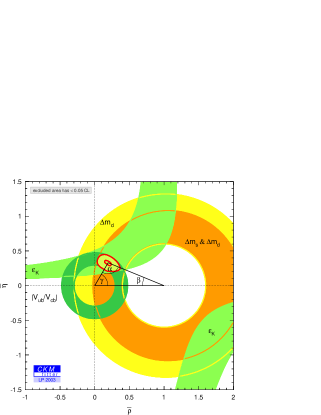
Figure 8: “Classic” experimental constraints on the $\rho-\eta$ plane. The circles centered at $(0,0)$ come from Eq. (177). The circles centered at $(1,0)$ come from Eq. (178): yellow for $\Delta m_{d}$, brown for the improvement due to $\Delta m_{s}$. The hyperbolic curves in green arise from Eq. (179). The intersection of all constraints (red curves) determines the region in the $\rho-\eta$ plane consistent with these experiments.

A few points should be noticed:

• the tests implicit in the rescaled unitarity triangle of Eq. (176) are also illustrated in FIG. 8;

• the sizable improvement provided when we utilize the lower bound on $\Delta m_{s}$;

• the agreement of all the allowed regions into a single overlap region means that these experiments by themselves are not enough to uncover new physics;

• the rather large allowed regions provided by each experiment individually, which are mainly due to theoretical uncertainties. As mentioned in the introduction, hadronic messy effects are our main enemy in the search for signals of new physics.

The improvement provided by $\Delta m_{s}$ is mostly due to the fact that the theoretical errors involved in extracting $|V_{tb}V_{tq}|$ from $\Delta m_{q}$ ($q$ = $d$, $s$) cancel partly in the ratio [65]

$$\frac{\Delta m_{s}}{\Delta m_{d}}=\frac{m_{B_{s}}}{m_{B_{d}}}\xi^{2}\left|\frac{V_{ts}}{V_{td}}\right|^{2}.$$ (180)

Here, $\xi=1.15\pm 0.05^{+0.12}_{-0.00}$ is an SU(3) breaking parameter obtained from lattice QCD calculations [66]. Thus, a measurement of $\Delta m_{s}$, when it becomes available from experiments at hadronic machines, will be very important in reducing the (mostly theoretical) uncertainties in the extraction of $R_{t}$.

The bounds discussed in this section carry somewhat large theoretical errors. As we will see shortly, the CP violating asymmetry in $B_{d}\rightarrow J/\psi K_{S}$ provides us with a very clean measurement of the CKM phase $\beta$. This was the first real test of the SM to come out of the $B$ factories.

6 On the road to $\lambda_{f}$

In chapter 4 we saw that CP violation in the decays of neutral $B$ mesons may be described by a phenomenological parameter $\lambda_{f}$. In chapter 5 we reviewed the SM; a specific theory of electroweak interactions. This theory will now be tested by calculating $\lambda_{f}$ for a variety of final states and confronting its parameters (most notably $\rho$ and $\eta$) with those experiments. A few of the following sections were designed to avoid the common potholes on that road.

6.1 Can we calculate $q/p$?

As we have seen in subsection 3.2.2 and in section 4.4, when studying large CP violating effects in $B$ meson decays, we may assume $|\Gamma_{12}|\ll|M_{12}|$ and CP conservation in $B-\overline{B}$ mixing. As a result,

$$\frac{q_{B}}{p_{B}} = -\eta_{B}e^{i\xi},$$ (181)

$$= -\sqrt{\frac{M_{12}^{\ast}}{M_{12}}},$$ (182)

where $\xi$ is the arbitrary CP transformation phase in

$${\cal CP}|B^{0}_{q}\rangle = e^{i\xi}|\overline{B^{0}_{q}}\rangle,$$ (183)

$${\cal CP}|\overline{B^{0}_{q}}\rangle = e^{-i\xi}|B^{0}_{q}\rangle.$$ (184)

The parameter $\eta_{B}=\pm 1$ appears in ${\cal CP}|B_{H}\rangle=\eta_{B}|B_{H}\rangle$, consistently with the fact that, if there is CP conservation in the mixing, then the eigenstates of the Hamiltonian must also be CP eigenstates. In the SM, and when neglecting CP violation, one obtains $\eta_{B}=-1$, meaning that the heavier state is CP odd in that limit.

Having reached this point, it is tempting to “parametrize” the phase of $M_{12}$ within a given model and with “suitable phase choices” to be $e^{-2i\phi_{M}}$. One then concludes from Eq. (182) that

$$\frac{q_{B}}{p_{B}}=-\eta_{B}e^{2i\phi_{M}},$$ (185)

where $\phi_{M}$ would be some measurable phase. For instances, in the SM one would obtain $\frac{q_{B}}{p_{B}}=e^{-2i\beta}$. Strictly speaking, this is wrong, because it is at odds with Eq. (181); i.e., it contradicts the quantum mechanical rule that, when CP is conserved in mixing, the eigenstates of the Hamiltonian should coincide with the eigenstates of CP.

Let us use Eq. (182) to perform a correct calculation of $q_{B}/p_{B}$ [67]. The quantity $M_{12}$ is calculated from an effective Hamiltonian having a weak (CP odd) phase $-2\phi_{M}$, and a $\Delta B=2$ operator ${\cal O}$:

$$M_{12} = e^{-2i\phi_{M}}\langle B^{0}_{q}|{\cal O}|\overline{B^{0}_{q}}\rangle,$$

$$M_{12}^{\ast} = e^{2i\phi_{M}}\langle\overline{B^{0}_{d}}|{\cal O}^{\dagger}|B^{0}_{q}\rangle.$$ (186)

The operator ${\cal O}$ and its Hermitian conjugate are related by the CP transformation

$$\left({\cal CP}\right){\cal O}^{\dagger}\left({\cal CP}\right)^{\dagger}=e^{2i\xi_{M}}{\cal O}.$$ (187)

We may use two insertions of $\left({\cal CP}\right)^{\dagger}\left({\cal CP}\right)=1$ in the second Eq. (186) to derive

$$M_{12}^{\ast} = e^{2i\phi_{M}}\langle\overline{B^{0}_{q}}|\left({\cal CP}\right)^{\dagger}\left({\cal CP}\right){\cal O}^{\dagger}\left({\cal CP}\right)^{\dagger}\left({\cal CP}\right)|B^{0}_{q}\rangle$$ (188)

$$= e^{2i\left(\phi_{M}+\xi+\xi_{M}\right)}\langle B^{0}_{q}|{\cal O}|\overline{B^{0}_{q}}\rangle$$

$$= e^{2i\left(2\phi_{M}+\xi+\xi_{M}\right)}M_{12}.$$

Then, from Eq. (182),

$$\frac{q_{B}}{p_{B}}=-\eta_{B}e^{i\left(2\phi_{M}+\xi+\xi_{M}\right)}.$$ (189)

This should be equal to $-\eta_{B}e^{i\xi}$, as in Eq. (181). The CP transformation phase $\xi_{M}$ must therefore be chosen such that $2\phi_{M}+\xi_{M}=0$.

How does that come about? Let us illustrate this point with the calculation of $q_{B}/p_{B}$ within the SM. There,

$${\cal O}\propto\left[\overline{q}\gamma^{\mu}\left(1-\gamma_{5}\right)b\right]\left[\overline{q}\gamma_{\mu}\left(1-\gamma_{5}\right)b\right],$$ (190)

and

$$e^{-2i\phi_{M}}=\frac{V_{tb}V_{tq}^{\ast}}{V_{tb}^{\ast}V_{tq}}=\left\{\begin{array}[]{llr}e^{-2i\beta}&\ \ \mbox{for}&B_{d},\\ e^{2i\chi}&\ \ \mbox{for}&B_{s}.\end{array}\right.$$ (191)

Now, in the mass basis, the most general CP transformation of the quark fields $b$ and $q$ is, according to Eqs. (137),

$$\left({\cal CP}\right)b\left({\cal CP}\right)^{\dagger} = e^{i\xi_{b}}\gamma^{0}C\overline{b}^{T},$$

$$\left({\cal CP}\right)\overline{q}\left({\cal CP}\right)^{\dagger} = -e^{-i\xi_{q}}q^{T}C^{-1}\gamma^{0}.$$ (192)

Then, from Eqs. (190) and (187), $\xi_{M}=\xi_{q}-\xi_{b}$ and

$$\frac{q_{B}}{p_{B}}=-\eta_{B}e^{i(\xi+\xi_{q}-\xi_{b})}\frac{V_{tb}^{\ast}V_{tq}}{V_{tb}V_{tq}^{\ast}}.$$ (193)

The requirement that $2\phi_{M}+\xi_{M}=0$ is equivalent to

$$V_{tb}V_{tq}^{\ast}=e^{i\left(\xi_{q}-\xi_{b}\right)}V_{tb}^{\ast}V_{tq}.$$ (194)

It is clear that we may always choose $\xi_{q}$ and $\xi_{b}$ such that Eq. (194) be verified, thus obtaining CP invariance. We recognize Eq. (194) as resulting from Eq. (139), which expresses CP conservation in the SM. We conclude from this particular example that, when one discards the free phases in the CP transformation of the quark fields, one may occasionally run into contradictions.

But now we have another problem. If Eq. (181) holds in any model leading to CP conservation in mixing, and since $\xi$ is an arbitrary phase, what does it mean to calculate $\lambda_{f}$?

6.2 Cancellation of the CP transformation phases in $\lambda_{f}$

Let us consider the decays of $B^{0}_{q}$ and $\overline{B^{0}_{q}}$ into a CP eigenstate $f_{\rm cp}$:

$${\cal CP}|f_{\rm cp}\rangle=\eta_{f}|f_{\rm cp}\rangle,$$ (195)

with $\eta_{f}=\pm 1$. We assume that the decay amplitudes have only one weak phase $\phi_{A}$, with an operator ${\cal O}^{\prime}$ controlling the decay,

$$A_{f} = e^{i\phi_{A}}\langle f_{\rm cp}|{\cal O}^{\prime}|B^{0}_{q}\rangle,$$

$$\bar{A}_{f} = e^{-i\phi_{A}}\langle f_{\rm cp}|{{\cal O}^{\prime}}^{\dagger}|\overline{B^{0}_{q}}\rangle.$$ (196)

The CP transformation rule for ${\cal O}^{\prime}$ is

$$\left({\cal CP}\right){{\cal O}^{\prime}}^{\dagger}\left({\cal CP}\right)^{\dagger}=e^{-i\xi_{D}}{\cal O}^{\prime}.$$ (197)

Then,

$$\bar{A}_{f} = e^{-i\phi_{A}}\langle f_{\rm cp}|\left({\cal CP}\right)^{\dagger}\left({\cal CP}\right){{\cal O}^{\prime}}^{\dagger}\left({\cal CP}\right)^{\dagger}\left({\cal CP}\right)|\overline{B^{0}_{q}}\rangle$$ (198)

$$= \eta_{f}e^{-i\left(\phi_{A}+\xi+\xi_{D}\right)}\langle f_{\rm cp}|{\cal O}^{\prime}|B^{0}_{q}\rangle$$

$$= \eta_{f}e^{-i\left(2\phi_{A}+\xi+\xi_{D}\right)}A_{f}.$$

Combining Eq. (189) and (198), we obtain

$$\lambda_{f}\equiv\frac{q_{B}}{p_{B}}\frac{\bar{A}_{f}}{A_{f}}=-\eta_{B}\eta_{f}e^{2i(\phi_{M}-\phi_{A})}e^{i(\xi_{M}-\xi_{D})}.$$ (199)

We now state the following: if the calculation has been done correctly, then the phases $\xi_{M}$ and $\xi_{D}$, which arise in the CP transformation of the mixing and decay operators, are equal and cancel out. This cancellation is due to the fact that, because they involve the same quark fields, the CP transformation properties of the $\Delta B=2$ operators describing the mixing are related to those of the $\Delta B=1$ operators describing the decay. Thus,

$$\lambda_{f}=-\eta_{B}\eta_{f}e^{2i(\phi_{M}-\phi_{A})}.$$ (200)

An explicit example of the cancellation of the CP transformation phases occurs in the SM computation of the parameter $\lambda_{f}$, as shown in chapter 33 of reference [1] for a variety of final states. Below we will check this cancellation explicitly for the decay $B_{d}\rightarrow J/\psi K_{S}$.

There are two important points to note in connection with Eq. (200):

• If we had set $\xi_{M}=\xi_{D}=0$ from the very beginning we would have obtained the correct result for $\lambda_{f}$. This is what most authors do. The price to pay is, as pointed out above, an inconsistency between Eqs. (185) and (181).

• The $-\eta_{B}=\mp 1$ sign in Eq. (200) is important. That sign comes from $q_{B}/p_{B}$ in Eq. (181). And, to be precise, the sign of $q_{B}/p_{B}$ is significant only when compared with the sign of either $\Delta m$ or $\Delta\Gamma$. Therefore, it is not surprising to find that $\lambda_{f}$ always appears multiplied by an odd function of either $\Delta m$ or $\Delta\Gamma$ in any experimental observable, c.f. Eqs. (91) and (97).

6.3 A common parametrization for mixing and decay within a given model

Having realized where contradictions might (and do) arise and that the calculations of $\lambda_{f}$ are safe, we will now brutally simplify the discussion by ignoring the “spurious” phases brought about by CP transformations,

Let us consider the decay $B^{0}_{d}\rightarrow f_{\rm cp}$, mediated by two diagrams with magnitudes $A_{1}$ and $A_{2}$, CP odd phases (weak-phases) $\phi_{A1}$ and $\phi_{A2}$, and CP even phases (strong phases) $\delta_{1}$ and $\delta_{2}$. Let us take $\phi_{M}$ as the CP odd phase in $B^{0}_{d}-\overline{B^{0}_{d}}$ mixing. Then,

$$\frac{q_{B}}{p_{B}} = -\eta_{B}e^{2i\phi_{M}}\ ,$$ (201)

$$A_{f} = A_{1}e^{i\phi_{A1}}e^{i\delta_{1}}+A_{2}e^{i\phi_{A2}}e^{i\delta_{2}}\ ,$$ (202)

$$\bar{A}_{f} = \eta_{f}\left(A_{1}e^{-i\phi_{A1}}e^{i\delta_{1}}+A_{2}e^{-i\phi_{A2}}e^{i\delta_{2}}\right)\ ,$$ (203)

from which

$$\lambda_{f}=-\eta_{B}\eta_{f}e^{-2i\phi_{1}}\frac{1+re^{i(\phi_{1}-\phi_{2})}e^{i\delta}}{1+re^{-i(\phi_{1}-\phi_{2})}e^{i\delta}}\ ,$$ (204)

where $\eta_{B}=\pm 1$, $\eta_{f}=\pm 1$, $\phi_{1}\equiv\phi_{A1}-\phi_{M}$, $\phi_{2}\equiv\phi_{A2}-\phi_{M}$, $\delta=\delta_{2}-\delta_{1}$ and $r=A_{2}/A_{1}$.

In a model, such as the Standard Model, the CP odd phases are determined by the weak interaction and are easily read off from the fundamental Lagrangian. In contrast, the CP even phases are determined by the strong interactions (and, on occasion, the electromagnetic interactions) and involve the calculation of hadronic matrix elements, including the final state interactions. These are usually calculated within a model of the hadronic interactions. Naturally, such calculations depend on the model used and, therefore, these quantities and the studies associated with them suffer from the corresponding “hadronic uncertainties”. Therefore, we are most interested in decays for which these hadronic uncertainties are small, or, in the limit, nonexistent.

6.3.1 Decays mediated by a single weak phase

This case includes those situations in which the decay is mediated by a single diagram ($r=A_{2}/A_{1}=0$) as well as those situations in which there are several diagrams mediating the decay, but all share the same weak phase ($\phi_{1}-\phi_{2}=\phi_{A1}-\phi_{A2}=0$). Then

$$\lambda_{f}=-\eta_{B}\eta_{f}e^{-2i\phi_{1}},$$ (205)

from which $|\lambda_{f}|=1$, and Eqs. (93) and (94) yield

$$C_{f} = 0\ ,$$ (206)

$$S_{f} = \eta_{B}\eta_{f}\sin{2\phi_{1}}\ .$$ (207)

These are clearly ideal decays, because the corresponding CP asymmetry depends on a single weak phase (which may be calculated in the Standard Model as well as other models); it does not depend on the strong phases, nor on the magnitudes of the decay amplitudes (meaning that these asymmetries do not depend on the hadronic uncertainties.) Therefore, the search for CP violating asymmetries in decays into final states which are eigenstates of CP and whose decay involves only one weak phase constitutes the Holy Grail of CP violation in the $B$ system.

6.3.2 Decays dominated by one weak phase

Unfortunately, most decays involve several diagrams, with distinct weak phases. To understand the devious effect that a second weak phase has, it is interesting to consider the case in which, although there are two diagrams with different weak phases, the magnitudes of the corresponding decay amplitudes obey a steep hierarchy $r<<1$. In that case, Eqs. (93) and (94) yield (Ex-28)

$$C_{f} \approx 2r\sin{(\phi_{1}-\phi_{2})}\sin{\delta}\ ,$$ (208)

$$S_{f} \approx \eta_{B}\eta_{f}\left[\sin{2\phi_{1}}-2r\cos{2\phi_{1}}\sin{(\phi_{1}-\phi_{2})}\cos{\delta}\right]\ .$$ (209)

These equations allow us to learn a few important lessons.

First, the CP violation present in the decays (direct CP violation) is only non-zero if

• there are at least two diagrams mediating the decay;

• these two diagrams have different weak phases;

• and these two diagrams also have different strong phases.

On the other hand, since it depends on $r$ and $\delta$, the calculation of the direct CP violation parameter $C_{f}$ depends always on the hadronic uncertainties. These features do not depend on the $r$ expansion which we have used; they are valid in all generality and hold also for the direct CP violation probed with $B^{\pm}$ decays.

Second, when we have two diagrams involving two distinct weak phases, the interference CP violation also becomes dependent on $r$ and $\delta$. As a result, the calculation of $S_{f}$ is also subject to hadronic uncertainties. Notice that, for $S_{f}$, this problem is worse than it seems. Indeed, even if the final state interactions are very small (in which case $\delta\sim 0$, and $C_{f}\sim 0$ does not warn us about the presence of a second weak phase.), $S_{f}$ will still depend on $r$ [68]. That is, the presence of a second amplitude with a different weak phase can destroy the measurement of $\sin 2\phi_{1}$, even when the strong phase difference vanishes. This problem occurs even for moderate values of $r$.

To simplify the discussion, we could say that some $B$ decays we are interested in have both a tree level diagram and a gluonic penguin diagram, which is higher order in perturbation theory. As such, we could expect that $r=A_{2}/A_{1}<1$. However, this might not be the case, both because the tree level diagram might be suppressed by CKM mixing angles, and because the decay amplitudes involve hadronic matrix elements which, in some cases, are difficult to estimate. For this purpose, it is convenient to write $r=r_{\rm ckm}r_{h}$, where $r_{\rm ckm}$ is the ratio of the magnitudes of the CKM matrix elements in the two diagrams. We can now separate two possibilities, according to the size of $r_{\rm ckm}\sin{(\phi_{1}-\phi_{2})}$ [69]:

1. if $r_{\rm ckm}\sin{(\phi_{1}-\phi_{2})}\ll 1$, then combining this with some rough argument that $r_{h}$ is small will allow us to conclude that $r\sin{(\phi_{1}-\phi_{2})}\ll 1$, and $S_{f}\approx\eta_{B}\eta_{f}\sin{2\phi_{1}}$;

2. if $r_{\rm ckm}\sin{(\phi_{1}-\phi_{2})}\sim 1$, then we must really take the second weak phase into account, because any rough argument about the “smallness” of $r_{h}$, by itself, will not guarantee that the error introduced by $r\sin{(\phi_{1}-\phi_{2})}$ will indeed be small.

An exhaustive search shows that the best case occurs for $B_{d}\rightarrow J/\psi K_{S}$.

7 $B$ decays as a test of the Standard Model

The interest in $B$ decays had its origin in the seminal articles by Carter and Sanda [70] and by Bigi and Sanda [71]. They identified early on the decay $B_{d}\rightarrow J/\psi K_{S}$ as a prime candidate in the search for CP violation outside the kaon system.

7.1 The decay $B_{d}\rightarrow J/\psi K_{S}$

7.1.1 Rephasing invariance, reciprocal basis, and other details

Although this is the most famous $B$ decay, its calculation is fraught with hazardous details:

1. $J/\psi K_{S}$ is not a CP eigenstate, given that $K_{S}$ itself is not a CP eigenstate. However, ignoring this detail does not affect our conclusions, because $\delta_{K}\sim 10^{-3}$ may be neglected with respect to the CP violating asymmetry of order unity present in $B_{d}\rightarrow J/\psi K_{S}$.

2. In some sense, $K_{S}$ is not even a good final state, since what we detect are its decay products $\pi^{+}\pi^{-}$. Now, it is clear that by selecting those events in which the kaon lives for proper times much greater than $\tau_{S}$, the $K_{S}$ component will have decayed away, and what one really measures is $K_{L}$. Therefore, the correct calculation must consider both paths of the cascade decay: $B_{d}\rightarrow J/\psi K_{S}\rightarrow J/\psi(\pi^{+}\pi^{-})$ and $B_{d}\rightarrow J/\psi K_{L}\rightarrow J/\psi(\pi^{+}\pi^{-})$ [72]. Of course, this effect is negligible for the small kaon decay times used in extracting $B_{d}\rightarrow J/\psi K_{S}$ data.

3. In the spectator quark approximation, the SM only allows the decays $B^{0}_{d}\rightarrow J/\psi K^{0}$ and $\overline{B^{0}_{d}}\rightarrow J/\psi\overline{K^{0}}$. The decay $B_{d}\rightarrow J/\psi K_{S}$ is only possible due to $K^{0}-\overline{K^{0}}$ mixing, which must be taken into account through [1]

   $$\frac{q_{K}}{p_{K}}=-\eta_{K}e^{i(\xi_{K}+\xi_{d}-\xi_{s})}\frac{V_{us}^{\ast}V_{ud}}{V_{us}V_{ud}^{\ast}}.$$ (210)

4. Although we will neglect CP violation in $K^{0}-\overline{K^{0}}$ mixing, we must use the reciprocal basis, or some expressions will be wrong.

5. Because the vector meson $J/\psi$ and the kaon arise from a $B$ decay, they must be in a relative $l=1$ state, which upon a CP (P) transformation yields an extra minus sign.

We may now combine the last three remarks into the calculation of $\lambda_{B_{d}\rightarrow J/\psi K_{S}}$.

As we have mentioned in section 3.3, when dealing with a $K_{S}$ in the final state we must use the reciprocal basis

$$\langle\tilde{K}_{S}|=\frac{1}{2p_{K}}\langle K^{0}|+\frac{1}{2q_{K}}\langle\overline{K^{0}}|.$$ (211)

Therefore,

$$\langle J/\psi\tilde{K}_{S}|T|B^{0}_{d}\rangle = \frac{1}{2p_{K}}\langle J/\psi K^{0}|T|B^{0}_{d}\rangle,$$

$$\langle J/\psi\tilde{K}_{S}|T|\overline{B^{0}_{d}}\rangle = \frac{1}{2q_{K}}\langle J/\psi\overline{K^{0}}|T|\overline{B^{0}_{d}}\rangle,$$ (212)

leading to

$$\lambda_{B_{d}\rightarrow J/\psi K_{S}}=\frac{q_{B}}{p_{B}}\frac{\bar{A}_{J/\psi K_{S}}}{A_{J/\psi K_{S}}}=\frac{q_{B}}{p_{B}}\frac{\langle J/\psi\overline{K^{0}}|T|\overline{B^{0}_{d}}\rangle}{\langle J/\psi K^{0}|T|B^{0}_{d}\rangle}\frac{p_{K}}{q_{K}}.$$ (213)

The presence of $p_{K}/q_{K}$ expresses the fact that the interference can only occur due to $K^{0}-\overline{K^{0}}$ mixing.

The mixing parameters are shown in Eqs. (193) and (210). We must now turn to the decay amplitudes. We start by assuming that the decay is mediated only by the tree level diagram in FIG. 9.

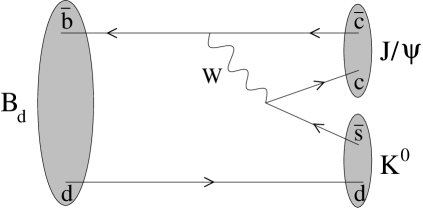
Figure 9: Tree level diagram for $B_{d}\rightarrow J/\psi K_{S}$.

Then

$$\langle J/\psi K^{0}|T|B^{0}_{d}\rangle\propto V_{cb}^{\ast}V_{cs}\langle J/\psi K^{0}|\left[\overline{b}\gamma^{\mu}\left(1-\gamma_{5}\right)c\right]\left[\overline{c}\gamma_{\mu}\left(1-\gamma_{5}\right)s\right]|B^{0}_{d}\rangle.$$ (215)

We now use multiple insertions of $\left({\cal CP}\right)^{\dagger}\left({\cal CP}\right)=1$. Then

$$\langle J/\psi K^{0}|\left({\cal CP}\right)^{\dagger}=-e^{-i\xi_{K}}\langle J/\psi\overline{K^{0}}|,$$ (216)

where the minus sign appears because $J/\psi$ and $K$ are in a relative $l=1$ state. Also

$$\left({\cal CP}\right)\left[\overline{b}\gamma^{\mu}\left(1-\gamma_{5}\right)c\right]\left({\cal CP}\right)^{\dagger} = -e^{i(\xi_{c}-\xi_{b})}\left[\overline{c}\gamma_{\mu}\left(1-\gamma_{5}\right)b\right],$$

$$\left({\cal CP}\right)\left[\overline{c}\gamma_{\mu}\left(1-\gamma_{5}\right)s\right]\left({\cal CP}\right)^{\dagger} = -e^{i(\xi_{s}-\xi_{c})}\left[\overline{s}\gamma^{\mu}\left(1-\gamma_{5}\right)c\right],$$

$$\left({\cal CP}\right)|B^{0}_{d}\rangle = e^{i\xi_{B}}|\overline{B^{0}_{d}}\rangle.$$ (217)

We obtain

$$\frac{\langle J/\psi\overline{K^{0}}|T|\overline{B^{0}_{d}}\rangle}{\langle J/\psi K^{0}|T|B^{0}_{d}\rangle}=-e^{i(\xi_{K}-\xi_{B}+\xi_{b}-\xi_{s})}\frac{V_{cb}V_{cs}^{\ast}}{V_{cb}^{\ast}V_{cs}}.$$ (218)

Substituting Eqs. (193), (210), and (218) into Eq. (213), we find,

$$\lambda_{B_{d}\rightarrow J/\psi K_{S}} = -\eta_{B}e^{i(\xi_{B}+\xi_{d}-\xi_{b})}\frac{V_{tb}^{\ast}V_{td}}{V_{tb}V_{td}^{\ast}}\;(-\eta_{K})e^{-i(\xi_{K}+\xi_{d}-\xi_{s})}\frac{V_{us}V_{ud}^{\ast}}{V_{us}^{\ast}V_{ud}}\;(-)e^{i(\xi_{K}-\xi_{B}+\xi_{b}-\xi_{s})}\frac{V_{cb}V_{cs}^{\ast}}{V_{cb}^{\ast}V_{cs}}$$ (219)

$$= -\eta_{B}\eta_{K}\frac{V_{tb}^{\ast}V_{td}}{V_{tb}V_{td}^{\ast}}\;\frac{V_{us}V_{ud}^{\ast}}{V_{us}^{\ast}V_{ud}}\;\frac{V_{cb}V_{cs}^{\ast}}{V_{cb}^{\ast}V_{cs}}$$

$$= -e^{-2i(\beta-\chi^{\prime})}.$$

where Eq. (168) and $\eta_{B}=\eta_{K}=-1$ were used to obtain the last line. Notice the cancellation of the various spurious phases $\xi$ brought about by the CP transformations in going from the first to the second line; the result is manifestly rephasing invariant. The cancellation occurs both for the spurious phases involving the kets and bras, $\xi_{B}$ and $\xi_{K}$, and for the spurious phases involving the fields in the quark field operators, $\xi_{q}$, c.f. Eq. (5). The last cancellation involves the balance between the CP transformation properties of the $\Delta B=2$ mixing and the $\Delta B=1$ decay operators and provides an explicit example of the cancellation $\xi_{M}-\xi_{D}=0$ mentioned in section 6.2.

7.1.2 Simplified $q/p$ and new physics

These lengthy calculation involving the phases $\xi$ and fractions with $V^{\ast}V$ bilinears are very reassuring, but they are a very hefty price to pay for consistency between Eqs. (181) and (185). It would be much easier to ignore the CP transformation phases in Eqs. (193) and (210) and to substitute the phases of all CKM matrix elements by Eq. (168). We would obtain

$$\frac{q_{B}}{p_{B}} = e^{-2i\tilde{\beta}},$$ (220)

$$\frac{q_{K}}{p_{K}} = e^{-2i\chi^{\prime}}\sim 1.$$ (221)

The phase $\tilde{\beta}$ in Eq. (220) includes the possibility that there might be new physics contributions to the relevant phase in $B^{0}_{d}-\overline{B^{0}_{d}}$ mixing [73]. In the SM, $\tilde{\beta}$ coincides with the CKM phase $\beta$. Because $\delta_{K}\sim 10^{-3}$, $\chi^{\prime}$ is likely to be small in almost any new physics model [1], and we will ignore it. Similarly, we may take

$$\frac{q_{Bs}}{p_{Bs}}=e^{2i\tilde{\chi}},$$ (222)

where $\tilde{\chi}$ allows for new physics contributions to the relevant phase in $B^{0}_{s}-\overline{B^{0}_{s}}$ mixing. In the SM $\tilde{\chi}$ coincides with the CKM phase $\chi$.

Because we know that, in the end, the expression for $\lambda_{f}$ yields the same result, and because we know where the pitfall is, we will henceforth use Eqs. (220)–(222). It is trivial to reproduce the last line of Eq. (219) with this (Ex-29).

7.1.3 $B_{d}\rightarrow J/\psi K_{S}$ involves one weak phase

The decay $B_{d}\rightarrow J/\psi K_{S}$ is mediated by the tree level diagram in FIG. 9. But it also gets a contribution from FIG. 10.

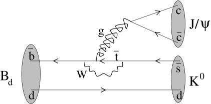
Figure 10: Penguin diagram with a virtual top quark which mediates the decay $B_{d}\rightarrow J/\psi K_{S}$. The gluonic line represents two or more gluons.

The two diagrams are proportional to

$$V_{cb}^{\ast}V_{cs} \sim (A\lambda^{2})(1),$$

$$V_{tb}^{\ast}V_{ts} \sim (1)(-A\lambda^{2}e^{i\chi}),$$ (223)

respectively, where we have used the parametrization in Eq. (169). The difference between the two weak phases is $\phi_{1}-\phi_{2}=\chi$ which, in the SM, is proportional to $\lambda^{2}$. On the other hand, since the penguin diagram is higher order in the weak interactions, we expect $r$ to be suppressed also. Therefore $r\sin{(\phi_{1}-\phi_{2})}\sim\lambda^{2}r$, the decay is overwhelmingly dominated by one weak phase, and Eq. (219) remains valid – possibly with $\tilde{\beta}$ in the place of $\beta$, to allow for the possibility of a new physics contribution to the phase in $B^{0}_{d}-\overline{B^{0}_{d}}$ mixing.

As a result, we conclude from Eqs. (93) – or (206) – that there is no direct CP violation in this decay, and that the interference CP violation term in Eqs. (94) – or (207) – is simply $S_{J/\psi K_{S}}=\sin{2\tilde{\beta}}$. The measurement of this parameter by BABAR and Belle constituted the first observation of CP violation outside the kaon system. It had to wait over 35 years! The PDG2004 world average is [17]

$$|\lambda_{B_{d}\rightarrow(c\bar{c})K}| = 0.949\pm 0.045\ ,$$ (224)

$$\sin{2\tilde{\beta}} = 0.731\pm 0.056\ ,$$ (225)

which provides an extremely precise constraint on a CKM parameter of the SM. The HFAG group has updated this result after the conferences of the summer of 2004, including all the charmonium states, obtaining $|\lambda_{B_{d}\rightarrow(c\bar{c})K}|=0.969\pm 0.028$ and $\sin{2\tilde{\beta}}=0.725\pm 0.037$ [55]. Recalling that $|\lambda_{f}|=|q_{B}/p_{B}||\bar{A}_{f}/A_{F}|$, Eq. (224) is consistent with very small or vanishing CP violation in both $B_{d}$ mixing and the $b\rightarrow c\bar{c}s$ decay amplitudes.

There are other diagrams contributing to the decay $B_{d}\rightarrow J/\psi K_{S}$, besides those in FIGs. 9 and 10. For example, we could use a virtual up quark instead of the virtual top quark in FIG. 10, which would seem to bring with it a third CKM combination $V_{ub}^{\ast}V_{us}$. However, due to the CKM unitarity relation in Eq. (171), we are still left with only two independent weak phases. Strictly speaking, one should refer to the operators multiplying each of the (chosen) two weak phases relevant for any particular decay, rather than to specific diagrams. This is elegantly included in the effective Hamiltonian approach [74]. However, the pictorial description of figures like FIGs. 9 and 10 provides a very intuitive idea of the mechanisms at hand in each decay.

7.1.4 Setting $\sin{2\beta}$ on the $\rho-\eta$ plane

In the SM, $\tilde{\beta}=\beta$ is related to the Wolfenstein parameters $\rho$ and $\eta$ through

$$\frac{1-\rho+i\eta}{\sqrt{(1-\rho)^{2}+\eta^{2}}}\approx e^{i\beta}.$$ (226)

Therefore, Eq. (225) corresponds to the area between two lines passing through $(\rho,\eta)=(1,0)$. Overlaying this constraint in FIG. 8, the CKMfitter group obtained, at the time of the conference LP2003, the result in FIG. 11 [64].

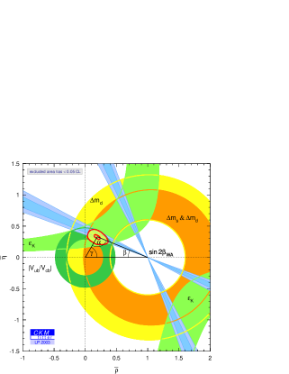
Figure 11: Constraints on the $\rho-\eta$ plane, with the results from $\sin{2\beta}$ overlaid.

The various blue areas shown correspond to a discrete ambiguity arising when one extracts $\beta$ from $\sin{2\beta}$.

Notice the perfect agreement of this measurement of $\sin{2\beta}$, in blue, with the results of FIG. 8 known previously. This is a major success for the SM, and it might well mean that the leading CP violating effects are dominated by the CKM mechanism. If so, we will need to combine a number of different experiments (preferably, with small theoretical uncertainties) in order to uncover new physics effects.

7.2 The penguin decay $B_{d}\rightarrow\phi K_{S}$ and related channels

The angle $\beta$ can be probed in a variety of decay channels. Performing those experiments allows us to “test the relation $\beta=\beta$”. Several candidates include:

• $b\rightarrow s\bar{s}s$ decays, such as $B_{d}\rightarrow\phi K_{S}$, $B_{d}\rightarrow\eta^{\prime}K_{S}$, and $B_{d}\rightarrow K^{+}K^{-}K_{S}$;

• $b\rightarrow c\bar{c}d$ decays, such as $B_{d}\rightarrow\psi\pi^{0}$, and $B_{d}\rightarrow D^{(\ast)\,+}D^{(\ast)\,-}$. Since the tree level amplitudes for these decays are suppressed by $\lambda$ with respect to the $b\rightarrow c\bar{c}s$, these will be more sensitive to new physics in $b\rightarrow d$ penguins than $b\rightarrow c\bar{c}s$ are to new physics in $b\rightarrow s$ penguins;

• $B_{d}\rightarrow AK_{S}$, where $A=\chi_{1},\eta_{c},\dots$ is some axial vector $c\bar{c}$ state. Comparing this with $B_{d}\rightarrow J/\psi K_{S}$ tests models which break P and CP [75];

• $B_{d}\rightarrow J/\psi K_{L}$. Comparing this with $B_{d}\rightarrow J/\psi K_{S}$, instead of including it in an overall $b\rightarrow c\bar{c}s$ analysis of $\tilde{\beta}$, allows for tests of CPT or of exotic $B_{d}^{0}\rightarrow\overline{K^{0}}$ decays [76, 77].

The decay $B_{d}\rightarrow\phi K_{S}$ is mediated by the penguin diagram in FIG. 12,

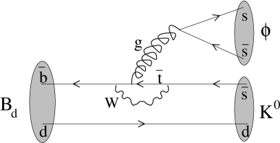
Figure 12: Penguin diagram with a virtual top quark which mediates the decay $B_{d}\rightarrow\phi K_{S}$. The gluonic line represents two or more gluons.

which should be compared with that involved in the decay $B_{d}\rightarrow J/\psi K_{S}$, shown in FIG. 10. Clearly, they share the CKM structure, shown on the second line of Eq. (223). As before, there is also a contribution from the penguin diagram with an intermediate charm quark, which involves the CKM structure shown on the first line of Eq. (223); and, using the CKM unitarity relation in Eq. (171), any other contribution may be written as a linear combination of these two. In contrast to the situation in the decay $B_{d}\rightarrow J/\psi K_{S}$, here there is no tree level contribution; this is a penguin decay. However, the relative phase between the two contributions is the same as in $B_{d}\rightarrow J/\psi K_{S}$; in the SM it is $\chi\sim\lambda^{2}$. Thus, four qualitative predictions are possible:

1. we also expect this decay to measure $\tilde{\beta}$, i.e.,

   $$\tilde{\beta}(\mbox{in}\ b\rightarrow s\ \mbox{penguin})=\tilde{\beta}(\mbox{in}\ b\rightarrow c\bar{c}s);$$ (227)

2. but, these $b\rightarrow s$ penguin decays are likely to be more affected by new physics than the tree level $b\rightarrow c\bar{c}s$ decays;

3. these new effects may both alter the interference CP violation, $S_{f}\neq\pm\sin{2\tilde{\beta}}$, and introduce CP violation in the decay, $C_{f}\neq 0$;

4. and, due to the different hadronic matrix elements involved, such new physics may have a different impact in different decays, such as $B_{d}\rightarrow\phi K_{S}$ and $B_{d}\rightarrow\eta^{\prime}K_{S}$.

The results at the time of the conference ICHEP2004 were [55]

$$C_{\phi K} = \left\{\begin{array}[]{ll}0.00\pm 0.23\pm 0.05&\mbox{BABAR}\\ -0.08\pm 0.22\pm 0.09&\mbox{Belle}\\ -0.04\pm 0.17&\mbox{HFAG average}\end{array}\ ,\right.$$ (231)

$$S_{\phi K} = \left\{\begin{array}[]{ll}+0.50\pm 0.25^{+0.07}_{-0.04}&\mbox{BABAR}\\ +0.06\pm 0.33\pm 0.09&\mbox{Belle}\\ +0.34\pm 0.20&\mbox{HFAG average}\end{array}\ .\right.$$ (235)

Recall that a sizable difference between $\sin{2\tilde{\beta}}$ extracted from $B_{d}\rightarrow J/\psi K_{S}$ and from $B_{d}\rightarrow\phi K_{S}$ is a problem for the SM. In 2003 $S_{\phi K}=-0.14\pm 0.33$ posed a serious problem (which now seems to be much reduced in this channel). This spurred a renewed interest in new physics contributions to this decay [78]. In general, attempts to reconcile $\sin{2\tilde{\beta}}\sim 0.73$ with a much smaller value for $S_{\phi K_{S}}$ involve new physics in $b\rightarrow s$ penguins; with amplitudes comparable to the SM; and with a large relative CP violating phase.

7.2.1 Enhanced electroweak penguins and small $S_{\phi K}$

One possibility consists in introducing non SM $sZb$ couplings through

$${\cal L}_{Z}^{\rm new}=\frac{g^{2}}{4\pi}\frac{g}{2\cos{\theta_{W}}}\left[Z_{sb}\ \bar{b}_{L}\gamma_{\mu}s_{L}+Z_{sb}^{\prime}\ \bar{b}_{R}\gamma_{\mu}s_{R}\right]\,Z^{\mu}+h.c.\ ,$$ (236)

where a loop-type suppression factor has been introduced in the definition of the coefficients $Z_{sb}$ and $Z_{sb}^{\prime}$. These couplings are already constrained by a number of observables, including the exclusive decay $B_{d}\rightarrow X_{s}e^{+}e^{-}$ [79], implying that the new $Z$ penguins are at most two to three times larger than the SM contributions to the decay $b\rightarrow s$.

Atwood and Hiller have used this possibility to illustrate an interesting point [75]. Consider the new physics diagram in FIG. 13, which competes with the SM one in FIG. 10.

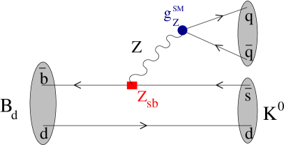
Figure 13: New diagram generated by the interactions in Eq. (236). For $q\bar{q}=s\bar{s}$ this contributes to the decay $B_{d}\rightarrow\phi K_{S}$; for $q\bar{q}=c\bar{c}$, this contributes to the decays $B_{d}\rightarrow(c\bar{c})K_{S}$. Notice the presence of the new $sZb$ coupling and of the SM coupling $g_{Z}^{\rm SM}$ in the $Zqq$ vertex.

When $q\bar{q}=s\bar{s}$ this contributes to the decay $B_{d}\rightarrow\phi K_{S}$, which might explain the discrepancy between the naive average of Eq. (235) and Eq. (225). But, when $q\bar{q}=c\bar{c}$, this contributes to the decays $B_{d}\rightarrow(c\bar{c})K_{S}$, thus altering the extraction of $\sin{2\tilde{\beta}}$. Now comes the important argument: because the SM $Zq\bar{q}$ coupling is involved, and because this coupling treats left and right handed quarks differently – c.f. Eq. (116) – it is crucial whether the $c\bar{c}$ quarks combine into a vector (V) or an axial-vector (A) meson. Indeed,

$$g_{Z}^{{\rm SM},V}(\psi,\psi^{\prime},\dots)=+0.19\ ,\hskip 56.9055ptg_{Z}^{{\rm SM},A}(\eta_{c},\chi_{1},\dots)=-0.5\ .$$ (237)

But this implies that comparing the value for $\sin{2\tilde{\beta}}$ extracted from $B_{d}\rightarrow(c\bar{c})\,K_{S}$ decays in which the $c\bar{c}$ quarks combine into a vector meson, with those obtained when the $c\bar{c}$ combine into an axial vector meson, will allow us to probe the type and parameter space of the new physics models proposed. A recent analysis [13] finds that the electroweak penguin explanation of an eventual discrepancy in this channel may be disfavored with respect to a modification of the gluonic penguins. Nevertheless, this important lesson remains: given two measurements of some quantity (say $\tilde{\beta}$) we should always ask what features of new physics models would be probed by a discrepancy in those measurements, and where else such features would show up. If the measurements show a clear sign of new physics, we throw a party; otherwise, we have a constraint on that class of models.

7.2.2 Tantalizing signals from $b\rightarrow s$ penguin decays

Things certainly heat up when we compare the results in Eq. (225), obtained from $b\rightarrow c\bar{c}s$ transitions, with the results obtained by comparing all $b\rightarrow s$ penguin decays. This is shown in HFAG’s FIG. 14 [55].

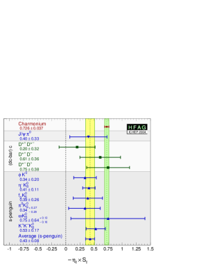
Figure 14: Experimental results for the interference CP violation parameter $S$ extracted from $b\rightarrow s$ penguin decays, compared with the results extracted with decays into charmonium states.

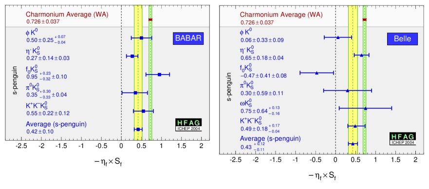
Figure 15: Experimental results for the interference CP violation parameter $S$ extracted from $b\rightarrow s$ penguin decays, compared with the results extracted with decays into charmonium states, as obtained by each experiment: BABAR Collaboration (left); Belle Collaboration (right).

The world averages after ICHEP2004 were [55]

$$C_{b\rightarrow s}=0.02\pm 0.05\ ,$$ (238)

$$S_{b\rightarrow s}=0.43\pm 0.08\ .$$ (239)

Although no signal is seen for direct CP violation, Eq. (239) differs from Eq. (225) by $3.6\sigma$. This is when we start paying attention.

This is all the more striking since this effect is clearly seen by both BABAR and Belle independently, as shown in HFAG’s FIG. 15. It is clear that $b\rightarrow s$ decays will be under close scrutiny during the next few years, both theoretically and experimentally.

7.3 The decay $B_{d}\rightarrow\pi^{+}\pi^{-}$ and related channels

7.3.1 Penguin pollution

The tree level and penguin diagrams affecting the decay $B_{d}\rightarrow\pi^{+}\pi^{-}$ are represented in FIGs. 16 and 17.

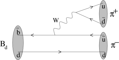
Figure 16: Tree level diagram for $B_{d}\rightarrow\pi^{+}\pi^{-}$.

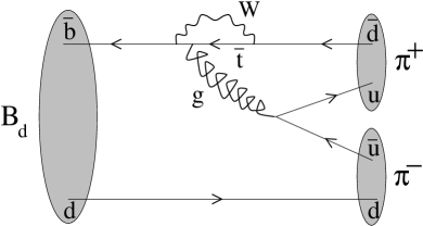
Figure 17: Penguin diagram with a virtual top quark which mediates the decay $B_{d}\rightarrow\pi^{+}\pi^{-}$. The gluonic line stands for any number of gluons.

These diagrams are proportional to

$$V_{ub}^{\ast}V_{ud} \approx \left(AR_{b}\lambda^{3}e^{i\gamma}\right)(1),$$

$$V_{tb}^{\ast}V_{td} \approx (1)\left(AR_{t}\lambda^{3}e^{-i\beta}\right),$$ (240)

respectively.

To understand the interest behind this decay, let us start by considering only the tree level diagram, neglecting the penguin diagram. If that were reasonable, then

$$\lambda_{B_{d}\rightarrow\pi^{+}\pi^{-}}=\frac{q_{B}}{p_{B}}\frac{\langle\pi^{+}\pi^{-}|T|\overline{B^{0}_{d}}\rangle}{\langle\pi^{+}\pi^{-}|T|B^{0}_{d}\rangle}=e^{-2i(\tilde{\beta}+\gamma)}.$$ (241)

Thus, if there were only tree level diagrams, the CP violating asymmetry in this decay would measure $\tilde{\beta}+\gamma$. Within the SM, this coincides with $\beta+\gamma$ and provides another constraint to be placed on the $\rho-\eta$ plane, thus improving our search for new physics. Since $\alpha=\pi-\beta-\gamma$ by definition, this is sometimes referred to as a measurement of $\alpha$. To highlight the fact that there are only two large phases in the CKM matrix, it may be preferable to view this as a measurement of $\tilde{\beta}+\gamma$. In models were the new physics is only in $B-\overline{B}$ mixing, $\tilde{\beta}$ is known from $B_{d}\rightarrow J/\psi K_{S}$, and $B_{d}\rightarrow\pi^{+}\pi^{-}$ provides a measurement of $\gamma$.

When both diagrams are taken into account

$$\lambda_{B_{d}\rightarrow\pi^{+}\pi^{-}}=e^{-2i\tilde{\beta}}\ \frac{e^{-i\gamma}\langle t\rangle+e^{i\beta}\langle p\rangle}{e^{i\gamma}\langle t\rangle+e^{-i\beta}\langle p\rangle}=e^{-2i(\tilde{\beta}+\gamma)}\ \frac{1+re^{i\delta}e^{i(\beta+\gamma)}}{1+re^{i\delta}e^{-i(\beta+\gamma)}},$$ (242)

where $\langle t\rangle$ ($\langle p\rangle$) contains the matrix element of the operator that appears multiplied by the CKM coefficient $V_{ub}^{\ast}V_{ud}$ ($V_{tb}^{\ast}V_{td}$), and the magnitude of that coefficient. Clearly, the terms proportional to

$$re^{i\delta}=\frac{\langle p\rangle}{\langle t\rangle},$$ (243)

where $r$ is a positive real number and $\delta$ a relative strong phase:

• destroy the simple relation in Eq. (241);

• imply that $\lambda_{B_{d}\rightarrow\pi^{+}\pi^{-}}$ is not a pure phase;

• and, because $re^{i\delta}$ depends crucially on the details of the hadronic matrix elements, such terms introduce a theoretical uncertainty into the interpretation of this experiment.

Indeed, for this decay, the difference between the two phases, $\phi_{1}-\phi_{2}=\gamma+\beta$, is large. Therefore, whatever convictions one might have about $r$, are not enough to guarantee that $C_{\pi^{+}\pi^{-}}$ vanishes or that $S_{\pi^{+}\pi^{-}}$ measures $-\sin{(2\tilde{\beta}+2\gamma)}$. The situation is made worse by the fact that $R_{b}\sim 0.4$ – Buras and Fleischer named this the $R_{b}$ suppression [80], – thus enhancing $r$. Gronau showed that this problem affects the measurement of $\tilde{\beta}+\gamma$, even for moderate values of $r$ [68]. This is known as “penguin pollution”.

7.3.2 Methods for trapping the penguin

The extraction of $\tilde{\beta}+\gamma$ from the CP asymmetry in $B_{d}\rightarrow\pi^{+}\pi^{-}$ would be straightforward if we were able to know $re^{i\delta}$; sometimes known as “trapping the penguin”. This may be achieved via two different paths: one may relate this decay to other decays invoking some symmetry property; or, one may try to calculate $re^{i\delta}$ directly within a given theoretical treatment of the hadronic interactions.

Some possibilities are listed below, where $\mbox{BR}_{\rm av}$ stands for the branching ratio averaged over a particle and its antiparticle.

• Gronau and London advocated the use of isospin [81] to relate the decay $B_{d}\rightarrow\pi^{+}\pi^{-}$ with the decays $B_{d}\rightarrow\pi^{0}\pi^{0}$ and $B^{+}\rightarrow\pi^{+}\pi^{0}$ through

  $$\frac{1}{\sqrt{2}}\langle\pi^{+}\pi^{-}|T|B^{0}_{d}\rangle+\langle\pi^{0}\pi^{0}|T|B^{0}_{d}\rangle=\langle\pi^{+}\pi^{0}|T|B^{+}\rangle.$$ (244)

  This method requires the measurement of

  $$\mbox{BR}_{\rm av}(\pi^{+}\pi^{-}),\ \ C_{\pi^{+}\pi^{-}},\ \ S_{\pi^{+}\pi^{-}},\ \ \mbox{BR}_{\rm av}(\pi^{0}\pi^{0}),\ \ C_{\pi^{0}\pi^{0}},\ \ \mbox{BR}_{\rm av}(\pi^{+}\pi^{0}).$$ (245)

  Of these, all have been available for some time, except for $C_{\pi^{0}\pi^{0}}$, which was only recently measured by BABAR to be $C_{\pi^{0}\pi^{0}}=-0.12\pm 0.56\pm 0.06$ [82], and by Belle to be $C_{\pi^{0}\pi^{0}}=-0.43\pm 0.51\pm 0.17$ [83]. This method determines $\tilde{\beta}+\gamma$ with a 16-fold ambiguity. If one were able to measure also $S_{\pi^{0}\pi^{0}}$, one would determine $\tilde{\beta}+\gamma$ with a 4-fold ambiguity.

• Grossman and Quinn pointed out that one may get some information even with a partial realization of the isospin analysis [84, 85, 86]. In its simplest form [84], this requires the measurement of

  $$C_{\pi^{+}\pi^{-}},\ \ S_{\pi^{+}\pi^{-}},\ \ \mbox{BR}_{\rm av}(\pi^{+}\pi^{0}),\ \ \mbox{upper bound on }\mbox{BR}_{\rm av}(\pi^{0}\pi^{0}).$$ (246)

• Silva and Wolfenstein proposed the use of flavor SU(3) – in fact, $U$-spin – to relate the decay $B^{0}_{d}\rightarrow\pi^{+}\pi^{-}$ with $B_{d}\rightarrow K^{+}\pi^{-}$ [87]. Indeed, the diagrams mediating the decay $B_{d}\rightarrow K^{+}\pi^{-}$ are obtained from those in FIGs. 16 and 17, which mediate the decay $B^{0}_{d}\rightarrow\pi^{+}\pi^{-}$, with the simple substitution of $\bar{d}\rightarrow\bar{s}$, leading to $\pi^{+}\rightarrow K^{+}$. The new diagrams are proportional to

  $$V_{ub}^{\ast}V_{us} \approx \left(AR_{b}\lambda^{3}e^{i\gamma}\right)(\lambda),$$

  $$V_{tb}^{\ast}V_{ts} \approx (1)\left(-A\lambda^{2}e^{-i\chi}\right),$$ (247)

  respectively. The crucial point behind this idea may be understood by comparing Eq. (247) with Eq. (240): the ratio $r$ in $B_{d}\rightarrow K^{+}\pi^{-}$ is enhanced by $1/\lambda^{2}$ with respect to the ratio $r$ in $B_{d}\rightarrow\pi^{+}\pi^{-}$. In fact, the $B_{d}\rightarrow K\pi$ decays are predicted to be penguin dominated, which makes them a very good source of information on the penguin needed to extract $\tilde{\beta}+\gamma$ from $B_{d}\rightarrow\pi^{+}\pi^{-}$ [87].

  In the simplest approximation [87], one needs only the measurements of

  $$\mbox{BR}_{\rm av}(\pi^{+}\pi^{-}),\ \ S_{\pi^{+}\pi^{-}},\ \ \mbox{BR}_{\rm av}(K^{+}\pi^{-}).$$ (248)

  Since then, a variety of other methods using $U$-spin to extract information from CP asymmetries have been proposed [88].

• One may also use some theoretical method in order to calculate the hadronic matrix elements required [89, 90, 91, 92, 93].

The first two methods, based on isospin, will be discussed in detail in subsection 7.3.5.

7.3.3 The $C-S$ plane

The PDG2004 world averages for the CP violating observables in the decay $B_{d}\rightarrow\pi^{+}\pi^{-}$ were [17]

$$C_{\pi^{+}\pi^{-}} = -0.51\pm 0.23\ ,$$

$$S_{\pi^{+}\pi^{-}} = -0.5\pm 0.6\ ,$$ (249)

which, after ICHEP2004, became [55]

$$C_{\pi^{+}\pi^{-}} = -0.37\pm 0.11\ (0.24)\ ,$$

$$S_{\pi^{+}\pi^{-}} = -0.61\pm 0.14\ (0.34)\ .$$ (250)

The inflated errors in between parenthesis result from the fact that the measurements of BABAR and Belle are inconsistent with each other. It is clear that a naive average is not the best procedure to combine inconsistent measurements, but how exactly this should be implement is the subject of some debate [94]. FIG. 18

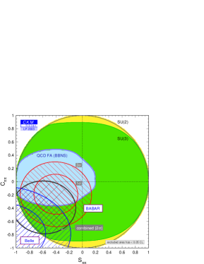
Figure 18: Experimental results for $B_{d}\rightarrow\pi^{+}\pi^{-}$ at the time of LP2003, compared with some theoretical analysis.

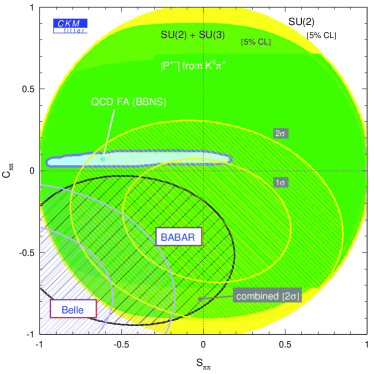
Figure 19: Experimental results for $B_{d}\rightarrow\pi^{+}\pi^{-}$ from data available in early 2003, compared with some theoretical analysis. Taken from [96].

shows an analysis made by the CKMfitter group [64] at the time of LP2003, where a later (rumored) result attributed to BABAR [95] had also been taken into account.

It is interesting to compare this with a similar FIG. 19, drawn by some members of the CKMfitter group at an earlier date [96]. Clearly, the experimental constraints have moved about within their error bars, as experimental results do. But the most remarkable feature is the enormous enlargement of the blue range obtained theoretically within the QCD factorization approach [89, 90, 91]. This is due to the fact that [90, 91] improved on the earlier analysis by including hard scattering spectator interactions $X_{H}$ and annihilation diagrams $X_{A}$, which cannot be estimated in a model independent fashion. As a result, one obtains larger CP even strong phases, thus enlarging considerably the $C_{\pi^{+}\pi^{-}}$ allowed range. Hadronic “messy” effects are really a nuisance.

7.3.4 $B_{d}\rightarrow\pi^{0}\pi^{0}$ and predictions from global fits

The methods mentioned in subsection 7.3.2 can be used in order to perform a global fit to all available data on two-body charmless $B$ decays. Because, typically, SU(2) introduces more parameters than there are data points, we are left with two classes of analysis:

1. Analysis utilizing a diagrammatic decomposition [88] based on SU(3) [97], in order to parametrize unknown matrix elements for different channels. Recent analysis may be found in [98] and [99, 100].

2. QCD based calculations of the hadronic matrix elements, in the context of perturbative QCD (pQCD) [92, 93], QCD factorization (QCDF) [89, 90, 91], and soft collinear effective theory (SCET) [101].

Before the experimental measurement of $\mbox{BR}_{\rm av}(\pi^{0}\pi^{0})$ was announced, global fits were performed in the context of U(3) [98], SU(3) [99], pQCD [93], and QCDF [91] with projections for this observable. I will name these “predictions”, because they appeared before the experimental results. The results are compiled in Table 1, together with the values for this branching ratio listed in PDG2004 [17] and improved at ICHEP2004.

pQCD	QCDF	SU(3)	U(3)	$\mbox{BR}_{\rm av}^{\rm exp}(\pi^{0}\pi^{0})$
$0.33-0.65$	$0.3\begin{array}[]{llll}+0.2&+0.2&+0.3&+0.2\\ -0.2&-0.1&-0.1&-0.1\end{array}$	$0.4-1.6$	$1.2-2.7$	$\begin{array}[]{ll}1.9\pm 0.5&\mbox{PDG2004}\\ 1.5\pm 0.3&\mbox{ICHEP04}\end{array}$

Table 1: Theoretical predictions for $\mbox{BR}_{\rm av}(\pi^{0}\pi^{0})$, compared with the experimental measurement, in units of $10^{-6}$.

The observation of this value for $\mbox{BR}_{\rm av}(\pi^{0}\pi^{0})$ has a few important consequences:

1. it enables the partial isospin, Grossman-Quinn bound;

2. it implies that $C_{\pi^{0}\pi^{0}}$ is within reach, thus enabling the full isospin analysis;

3. it poses a challenge to the QCD based predictions.

This is a rather difficult experiment, because there are no charged tracks. We must thank our experimentalist colleagues for their great efforts.

This decay is mediated by the tree level diagram in FIG. 20,

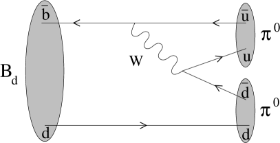
Figure 20: Color suppressed, tree level diagram for $B_{d}\rightarrow\pi^{0}\pi^{0}$.

which should be compared with the tree level diagram in FIG. 16. There, the $\bar{d}u$ quarks coming out of the (color singlet) $W$ go into the $\pi^{+}$ quark. Here, the $\bar{d}u$ quarks coming out of the (color singlet) $W$ go into two distinct mesons: the quark $\bar{d}$ must combine with the spectator $d$ to form a (color singlet) meson, although their colors are initially independent; and the quark $u$ must combine with the quark $\bar{u}$ from the other vertex to form a (color singlet) meson, although their colors are initially independent. Barring other effects, this entails a color suppression of the diagram in FIG. 20 (named “color suppressed”) with respect to that in FIG. 16 (named merely “tree”). Because it involves the color suppressed diagram in FIG. 20, the branching ratio for $B_{d}\rightarrow\pi^{0}\pi^{0}$ was suspected to be smaller than it turned out to be. Indeed, recent reanalysis including $\mbox{BR}_{\rm av}^{\rm exp}(\pi^{0}\pi^{0})$ into the fit, seem to require a rather large contribution from the color suppressed amplitude [13, 100], and a large strong phase relative to the tree (color allowed) diagram.

One final note before we proceed. Sometimes the connection between the two types of global fit mentioned, SU(3)-based and QCD-based, is a bit puzzling. Recently, in an extremely nice article, Bauer and Pirjol discussed the relation between the SU(3) diagrammatic decomposition and the matrix elements of operators used in the soft-collinear effective theory [102].

7.3.5 The isospin analysis in $B\rightarrow\pi\pi$ decays

In this section we discuss the isospin based methods utilized in the analysis of $B\rightarrow\pi\pi$ decays in more detail, separating it into small steps.

STEP 1: We start by recalling the definition of $C_{f}$ and defining a new quantity, $B^{f}$, proportional to the average decay width, as

$$C_{f} = \frac{|\bar{A}_{f}|^{2}-|A_{f}|^{2}}{|\bar{A}_{f}|^{2}-|A_{f}|^{2}},$$ (251)

$$B^{f} = \frac{|\bar{A}_{f}|^{2}+|A_{f}|^{2}}{2}.$$ (252)

The definitions for $C_{f}$ in Eqs. (93) and (251) coincide, because we are using $|q/p|=1$. Hence, the decay amplitudes are determined from the experimentally quoted values for the average branching ratios and decay CP violating parameters as

$$|\bar{A}_{f}|^{2} = B^{f}(1+C_{f}),$$

$$|A_{f}|^{2} = B^{f}(1-C_{f}).$$ (253)

STEP 2: Now, we parametrize the phase of $\lambda_{\pi^{+}\pi^{-}}$ by the difference $2\delta_{\alpha}$ from the value $2\alpha$ that it would have if there were only tree diagrams:

$$\lambda_{+-}\equiv\lambda_{\pi^{+}\pi^{-}}=|\lambda_{+-}|e^{2i(\alpha+\delta_{\alpha})}.$$ (254)

Since Eq. (93) leads to

$$\sqrt{1-C_{+-}^{2}}=\frac{2|\lambda_{+-}|}{1+|\lambda_{+-}|^{2}},$$ (255)

we find

$$S_{+-}=\frac{2\mbox{Im}(\lambda_{+-})}{1+|\lambda_{+-}|^{2}}=\sqrt{1-C_{+-}^{2}}\sin{(2\alpha+2\delta_{\alpha})}.$$ (256)

Surprising it may be, this is the crucial trick in the analysis by Grossman and Quinn [84].

STEP 3: In the limit of exact isospin symmetry, the two pions coming out of $B$ decays must be in an isospin $I=0$ or $I=2$ combination. Because gluons are isosinglet, they can only contribute to the $I=0$ final state. Therefore, the amplitude leading into the $I=2$ final state arises exclusively from tree level diagrams and, thus, it carries only one weak phase: $\gamma$. This is the crucial observation behind the Gronau–London method [81]. These issues are discussed in detail in (Ex-30), from which we take the isospin decomposition

$$\frac{1}{\sqrt{2}}A^{+-} \equiv \frac{1}{\sqrt{2}}\langle\pi^{+}\pi^{-}|T|B^{0}_{d}\rangle=T_{2}-A_{0},$$

$$A^{00} \equiv \langle\pi^{0}\pi^{0}|T|B^{0}_{d}\rangle=2\,T_{2}+A_{0},$$

$$A^{+0} \equiv \langle\pi^{+}\pi^{0}|T|B^{+}\rangle=3\,T_{2},$$ (257)

where we have used

$$A_{0} = \frac{1}{\sqrt{6}}A_{1/2},$$

$$T_{2} = \frac{1}{2\sqrt{3}}A_{3/2},$$ (258)

and the notation $T_{2}$ reminds us that this amplitude carries only the weak phase of tree level diagrams. Of course, there is a similar decomposition for the CP conjugated amplitudes:

$$\frac{1}{\sqrt{2}}\bar{A}^{+-} \equiv \frac{1}{\sqrt{2}}\langle\pi^{+}\pi^{-}|T|\overline{B^{0}_{d}}\rangle=\bar{T}_{2}-\bar{A}_{0},$$

$$\bar{A}^{00} \equiv \langle\pi^{0}\pi^{0}|T|\overline{B^{0}_{d}}\rangle=2\,\bar{T}_{2}+\bar{A}_{0},$$

$$\bar{A}^{+0}=A^{-0} \equiv \langle\pi^{-}\pi^{0}|T|B^{-}\rangle=3\,\bar{T}_{2}.$$ (259)

The first two amplitudes in Eq. (257) add up to the third one, the same happening with Eq. (259). This can be visualized as two triangles in the complex plane.

We will now follow the presentation of the Gronau–London method contained in [86]. Because $T_{2}$ only carries the weak phase $\gamma$, we may write it as

$$T_{2}=|T_{2}|e^{i\vartheta}e^{i\gamma},$$ (260)

where $\vartheta$ is a strong phase. As a result

$$\left(e^{2i\gamma}\right)\bar{T}_{2}=\left(e^{2i\gamma}\right)|T_{2}|e^{i\vartheta}e^{-i\gamma}=T_{2}.$$ (261)

This means that, rotating all sides of the CP conjugated triangle by the phase $2\gamma$,

$$\tilde{A}^{+-} = \left(e^{2i\gamma}\right)\bar{A}^{+-},$$

$$\tilde{A}^{00} = \left(e^{2i\gamma}\right)\bar{A}^{00},$$

$$\tilde{A}^{+0} = \left(e^{2i\gamma}\right)\bar{A}^{+0}=A^{+0},$$ (262)

makes the sides $\tilde{A}^{+0}=A^{+0}$ coincide. This is shown in FIG. 21,

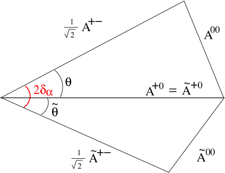
Figure 21: Isospin triangles utilized in the Gronau–London method.

where we define the angle $\theta$ ($\tilde{\theta}$) between $A^{+-}$ ($\tilde{A^{+-}}$) and $A^{+0}$. The isospin prediction that $|A^{+0}|=|\bar{A}^{+0}|$ can be probed by looking for CP violation in the decay $B^{+}\rightarrow\pi^{+}\pi^{0}$.

Clearly,

$$\cos{\theta} = \frac{|A^{+0}|^{2}+\frac{1}{2}|A^{+-}|^{2}-|A^{00}|^{2}}{\sqrt{2}|A^{+0}||A^{+-}|},$$

$$\cos{\tilde{\theta}} = \frac{|\tilde{A}^{+0}|^{2}+\frac{1}{2}|\tilde{A}^{+-}|^{2}-|\tilde{A}^{00}|^{2}}{\sqrt{2}|\tilde{A}^{+0}||\tilde{A}^{+-}|},$$ (263)

from which we can extract $\sin{\theta}$ and $\sin{\tilde{\theta}}$, up to their signs.

STEP 4: FIG. 21 also shows the phase $2\delta_{\alpha}$ as being the angle between $A^{+-}$ and $\tilde{A}^{+-}$. Indeed,

$$\lambda_{+-} = |\lambda_{+-}|e^{2i(\alpha+\delta_{\alpha})}=\frac{q_{B}}{p_{B}}\frac{\bar{A}^{+-}}{A^{+-}}$$ (264)

$$= e^{-2i\beta}\left(e^{-2i\gamma}e^{2i\gamma}\right)\frac{\bar{A}^{+-}}{A^{+-}}=e^{2i\alpha}\frac{\tilde{A}^{+-}}{A^{+-}},$$

proving that assertion.

Since any of two triangles in FIG. 21 could be inverted, $|\delta_{\alpha}|$ might equal $|\theta\pm\tilde{\theta}|$. It will be important below to note that the deviation of the phase of $\lambda_{+-}$ from the weak CKM phase $2\alpha$ is maximized when the two triangles lie on opposite sides, as in FIG. 21. So, we consider that case, for which $\delta_{\alpha}=\theta+\tilde{\theta}$, and

$$1-\sin^{2}{\delta_{\alpha}}=\cos{2\delta_{\alpha}}=\cos{\theta}\cos{\tilde{\theta}}-\sin{\theta}\sin{\tilde{\theta}}=\mbox{function}\left(B^{+0},B^{+-},C_{+-},B^{00},C_{00}\right).$$ (265)

We are now ready to understand the Gronau-London method [81]. Eqs. (253) and (263) imply that the measurements of $B^{+0}$, $B^{+-}$, $C_{+-}$, $B^{00}$, and $C_{00}$ determine (up to discrete ambiguities) $\theta$, $\tilde{\theta}$ and, thus, $\delta_{\alpha}$, through Eq. (265). Combining this with the additional measurement of the interference CP violation in the decay $B_{d}\rightarrow\pi^{+}\pi^{-}$, $S_{+-}$, into Eq. (256),

$$\sin(2\alpha+2\delta_{\alpha})=\frac{S_{+-}}{\sqrt{1-C^{2}_{+-}}},$$ (266)

yields $\alpha$. This is the Gronau-London method.

We may now ask what would happen if we were not able to measure $C_{00}$. In that case, we would have to assume the worse case scenario (maximum value) for $\delta_{\alpha}$. This means that we must take $\delta_{\alpha}=\theta+\tilde{\theta}$, as done above, and minimize the function in Eq. (265) with respect to $C_{00}$. One obtains [86]

$${C_{00}}_{\mbox{\small minimize}}=\frac{C_{+-}}{2}\frac{B^{+-}\left(\frac{1}{2}B^{+-}-B^{+0}-B^{00}\right)}{B^{00}\left(\frac{1}{2}B^{+-}+B^{+0}-B^{00}\right)},$$ (267)

from which

$$\cos{2\delta_{\alpha}}\geq\frac{\left(\frac{1}{2}B^{+-}+B^{+0}-B^{00}\right)^{2}-B^{+-}B^{+0}}{B^{+-}B^{+0}\sqrt{1-C^{2}_{+-}}}.$$ (268)

This constraint on the deviation of $S_{+-}/\sqrt{(}1-C^{2}_{+-})$ from $\sin{2\alpha}$ constitutes the Gronau-London-Sinha-Sinha bound, and it is the best we can do to constrain $\alpha$ if $C_{00}$ is not known.

This bound may be rewritten as

$$\cos{2\delta_{\alpha}}\geq\frac{1-2B^{00}/B^{+0}}{\sqrt{1-C^{2}_{+-}}}+\frac{\left(\frac{1}{2}B^{+-}-B^{+0}+B^{00}\right)^{2}}{B^{+-}B^{+0}\sqrt{1-C^{2}_{+-}}}.$$ (269)

Since the second term is positive, we reach [84, 85]

$$\cos{2\delta_{\alpha}}\geq\frac{1-2B^{00}/B^{+0}}{\sqrt{1-C^{2}_{+-}}},$$ (270)

which is an improvement due to Charles on the earlier result appearing in reference [84]

$$\cos{2\delta_{\alpha}}\geq 1-2B^{00}/B^{+0}.$$ (271)

This is the famous Grossman-Quinn bound, although their article also quotes another version of this bound, more refined [84].

The Grossman-Quinn bound in Eq. (271) would be extremely useful if it turned out that $B^{00}$ were very small, as originally expected due to the “color suppression” mentioned in connection with FIG. 20. That some such bound was possible is very easy to see by looking back at Eqs. (257). Indeed, in the exact limit $|A^{00}|=0$, we have $A_{0}=-2T_{2}$, from which we conclude that $A^{+-}=3T_{2}$ only carries the weak CKM phase $\gamma$. Thus, the deviation of $S_{+-}/\sqrt{(}1-C^{2}_{+-})$ from $\sin{2\alpha}$ is intimately connected with how large $B^{00}$ is, i.e., $B^{00}$ sets an upper bound on the penguin contribution. Including their recent measurement of $C_{\pi^{0}\pi^{0}}=-0.12\pm 0.56\pm 0.06$, BABAR finds $|\delta_{\alpha}|<30^{\circ}$ at $90\%$ C. L. [82].

7.3.6 The decay $B_{d}\rightarrow\rho^{+}\rho^{-}$

In principle, the isospin analysis discussed in subsection 7.3.5, including the Grossman-Quinn type bounds, is also applicable to the decays $B_{d}\rightarrow\rho\rho$. This could be complicated by the fact that the $\rho$ has three helicities, but it turns out that experiments measure the final state to be completely longitudinally polarized [103]. Such a final state is CP even, and the analysis can proceed as before.

The decays $B_{d}\rightarrow\rho\rho$ have one very important advantage over their $B_{d}\rightarrow\pi\pi$ counterparts; the stringent upper bound on $B_{d}\rightarrow\rho^{0}\rho^{0}$ means that, here, the Grossman-Quinn bound is very effective. Indeed [104],

$$\frac{\mbox{BR}_{\rm av}(\pi^{0}\pi^{0})}{\mbox{BR}_{\rm av}(\pi^{+}\pi^{-})}=0.33\pm 0.07\ ,$$ (272)

lead BABAR to $|\delta_{\alpha}|<30^{\circ}$ [82], while

$$\frac{\mbox{BR}_{\rm av}(\rho^{0}\rho^{0})}{\mbox{BR}_{\rm av}(\rho^{+}\rho^{-})}<0.04\ ,$$ (273)

at the $90\%$ C.L., already implies that $|\delta_{\alpha}|<11^{\circ}$ in the $B_{d}\rightarrow\rho\rho$ decays [103].

However, there are also two additional difficulties. Firstly, due to the finite width of the $\rho$ resonance, the identical particle symmetry invoked for $\pi\pi$ in order to exclude $I=1$ as a possible final state configuration needs to be altered [105]. In principle, the corrections will be of the order of $(\Gamma_{\rho}/m_{\rho})\sim 4\%$, but this effect deserves further attention. Secondly, there may be interference with non-resonant contributions to $B$ meson decays into four pions, and with other resonances yielding the same final state. These effects may be modeled and fitted for.

7.3.7 Dealing with discrete ambiguities

The CKMfitter’s FIG. 22, shows bounds on $\alpha$ at the time of LP2003, when no measurement of $C_{\pi^{0}\pi^{0}}$ was available.

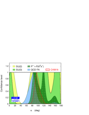
Figure 22: Extraction of $\alpha$ from $B_{d}\rightarrow\pi^{+}\pi^{-}$ with a variety of theoretical assumptions, compared with the result from the CKM fit (in red).

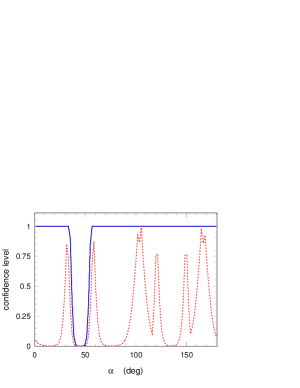
Figure 23: Toy exercise illustrating an SU(2) fit for $\alpha$, using putative, future experimental results excluding (red) or including (blue) a precise measurement of $C_{\pi^{0}\pi^{0}}$. (Extreme courtesy of A. Höcker [106].)

The SU(2) approach gave a very loose bound, corresponding roughly to the Grossman-Quinn bound. This is partly due to the lack of a precise measurement of $C_{\pi^{0}\pi^{0}}$. To illustrate the impact that a good measurement on this quantity would have, Höcker performed a very elucidative toy exercise just after LP2003 [106], shown in FIG. 23. He used the world averaged central values for $\mbox{BR}_{\rm av}(\pi^{+}\pi^{-})$, $\mbox{BR}_{\rm av}(\pi^{0}\pi^{0})$, and $\mbox{BR}_{\rm av}(\pi^{+}\pi^{0})$ and the BABAR central values for $C_{\pi^{+}\pi^{-}}$, $S_{\pi^{+}\pi^{-}}$, taking the errors to improve by a factor of five. Applying the Gronau-London method yields the curve in blue. Now, assume that the measurement of $C_{\pi^{0}\pi^{0}}$ was very precise, corresponding to $|\lambda_{B_{d}\rightarrow\pi^{0}\pi^{0}}|=1.00\pm 0.08$, just to see its impact. (All the numbers used in this exercise were utilized exclusively for illustrative purposes and need not be realistic.) Applying the Gronau-London method yields the curve in red. One sees the dramatic effect that a good measurement of $C_{\pi^{0}\pi^{0}}$ will have; it will allow us to see the eight discrete ambiguous solutions that the method yields for $\alpha$ in the interval $[0^{\circ},180^{\circ}]$. Fortunately, improved results for this observable are expected. This is the good news!

The bad news is that there are 1, 2, 3, …8, discretely ambiguous solutions for $\alpha$ in this interval. For the sake of argument, if all these solutions were separated, and each had an error of $10^{\circ}$, then we would have a $80^{\circ}$ allowed region for $\alpha$ in the interval $[0^{\circ},180^{\circ}]$. This is a major stumbling block in our search for new physics; new physics effects could be hiding behind any of these solutions and we wouldn’t know it. So, there are really two difficulties which must be dealt with in our search for new physics: hadronic “messy” elements; and discrete “smokescreen” ambiguities.

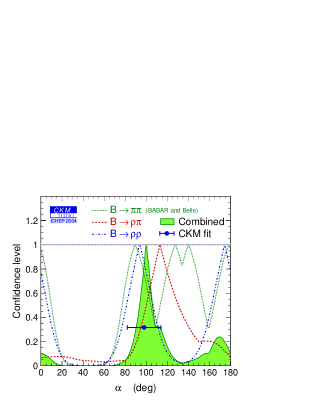
Figure 24: Extraction of $\alpha=\pi-\beta-\gamma$ from the decays $B_{d}\rightarrow\pi\pi$, $B_{d}\rightarrow\rho\pi$, and $B_{d}\rightarrow\rho\rho$. (Courtesy of A. Höcker.)

Now comes one of those intellectual twists that makes CP violation such an exciting field to work on: the presence of the first difficulty (hadronic effects) may help us resolve the second difficulty (discrete ambiguities). The simplified idea is the following: if there were no hadronic effects associated with the presence of the penguin diagram (which carries a weak phase that differs from the one in the tree level diagram), the CP violating asymmetry in the decay $B_{d}\rightarrow\pi^{+}\pi^{-}$ would probe only $S_{\pi^{+}\pi^{-}}$, which would equal $-\sin(2\beta+2\gamma)$. From this, one can extract $\beta+\gamma$, up to a four-fold discrete ambiguity. Were it not for the presence of hadronic effects, related decays might also provide $\sin(2\beta+2\gamma)$ and the same ambiguity might remain. Fortunately, the presence of hadronic effects shifts (and, in some cases, reduces the number of) the discrete ambiguities in the extraction of $\beta+\gamma$ in all decays. And this occurs differently for different decays, such as $B_{d}\rightarrow\rho\pi$ and $B_{d}\rightarrow\rho\rho$; each experiment gives a different set of discretely ambiguous solutions. Since the true solution to $\beta+\gamma$ must be common to all sets, we are able to exclude a number of “wrong” solutions. This can be seen clearly in FIG. 24 from the CKMfitter group [64], which combines the results from the decays $B_{d}\rightarrow\pi\pi$, $B_{d}\rightarrow\rho\pi$, and $B_{d}\rightarrow\rho\rho$, at the time of ICHEP2004. Notice the removal of many discrete ambiguities. Incidentally, this figure also shows that the extraction of $\beta+\gamma$ from these $b\rightarrow u$ decays is already competitive with the determination of $\beta+\gamma$ performed with the standard CKM fit.

7.4 $B\rightarrow K\pi$ decays

7.4.1 Diagrammatic decomposition and experimental results

In this section, we will concentrate on the decays in FIG. 25, which shows the diagrammatic decomposition discussed by Gronau and Rosner in [107, 108].

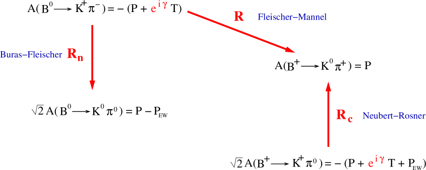
Figure 25: Simplified diagrammatic decomposition of $B\rightarrow K\pi$ decays. See text for details.

Here, $T$ and $P$ stand for the tree and gluonic penguin diagrams discussed above, while $P_{\rm EW}$ is an electroweak penguin; it is similar to the gluonic penguin, but with the gluon substituted by the $Z$-boson or the photon. Only the weak phase (which is $\gamma$) has been factored out explicitly. In analyzing exclusively $B\rightarrow K\pi$ decays, references [107, 108] include color suppressed (tree and electroweak penguins) through the redefinitions $P_{\rm EW}+C$, $T+P_{\rm EW}^{c}$, and $P-1/3\,P_{\rm EW}^{c}$. In the SU(3) decomposition, there exist other diagrams (with annihilation and exchange topologies) which have been neglected. A few features of FIG. 25 are immediately noticeable:

• if there were only gluonic penguin diagrams, then the decays with neutral pions in the final state would have about half the decay rate of those with charged pions in the final state;

• CP violation comes in with the tree diagram through the weak phase $\gamma$;

• the decays into neutral pions involve also the electroweak penguins $P_{\rm EW}$.

A lot can be learned from experiment by comparing these decays with each other. It is useful to define the ratios

$$R = \frac{\Gamma[B^{0}_{d}\rightarrow K^{+}\pi^{-}]+\Gamma[\overline{B^{0}_{d}}\rightarrow K^{-}\pi^{+}]}{\Gamma[B^{+}\rightarrow K^{0}\pi^{+}]+\Gamma[B^{-}\rightarrow\overline{K^{0}}\pi^{-}]}=\frac{\tau_{0}}{\tau_{+}}\frac{\mbox{BR}_{\rm av}(K^{+}\pi^{-})}{\mbox{BR}_{\rm av}(K^{0}\pi^{+})},$$ (274)

$$R_{c} = 2\frac{\Gamma[B^{+}\rightarrow K^{+}\pi^{0}]+\Gamma[B^{-}\rightarrow K^{-}\pi^{0}]}{\Gamma[B^{+}\rightarrow K^{0}\pi^{+}]+\Gamma[B^{-}\rightarrow\overline{K^{0}}\pi^{-}]}=2\frac{\mbox{BR}_{\rm av}(K^{+}\pi^{0})}{\mbox{BR}_{\rm av}(K^{0}\pi^{+})},$$ (275)

$$R_{n} = \frac{1}{2}\frac{\Gamma[B^{0}_{d}\rightarrow K^{+}\pi^{-}]+\Gamma[\overline{B^{0}_{d}}\rightarrow K^{-}\pi^{+}]}{\Gamma[B^{0}_{d}\rightarrow K^{0}\pi^{0}]+\Gamma[\overline{B^{0}_{d}}\rightarrow\overline{K^{0}}\pi^{0}]}=\frac{1}{2}\frac{\mbox{BR}_{\rm av}(K^{+}\pi^{-})}{\mbox{BR}_{\rm av}(K^{0}\pi^{0})},$$ (276)

first introduced by Fleischer and Mannel [109], Neubert and Rosner [110], and Buras and Fleischer [111], respectively.

The experimental results for the corresponding branching ratios (averaged over CP conjugated channels) and CP asymmetries at the time of LP2003, quoted in reference [108], are shown in Table 2. Also shown, between parenthesis, are the updated results from ICHEP 2004 quoted in [104].

Decay mode	$10^{6}\times\mbox{BR}_{\rm av}$ $\begin{array}[]{c}\mbox{at LP2003}\\ \mbox{(at ICHEP2004)}\end{array}$	$A_{\rm CP}$
$B^{+}\rightarrow K^{0}\pi^{+}$	$\begin{array}[]{c}21.78\pm 1.40\\ (24.1\pm 1.3)\end{array}$	$\begin{array}[]{c}0.016\pm 0.057\\ (-0.02\pm 0.03)\end{array}$
$B^{+}\rightarrow K^{+}\pi^{0}$	$\begin{array}[]{c}12.82\pm 1.07\\ (12.1\pm 0.8)\end{array}$	$\begin{array}[]{c}0.00\pm 0.12\\ (0.04\pm 0.04)\end{array}$
$B^{0}_{d}\rightarrow K^{+}\pi^{-}$	$\begin{array}[]{c}18.16\pm 0.79\\ (18.2\pm 0.8)\end{array}$	$\begin{array}[]{c}-0.095\pm 0.029\\ (-0.11\pm 0.02)\end{array}$
$B^{0}_{d}\rightarrow K^{0}\pi^{0}$	$\begin{array}[]{c}11.92\pm 1.44\\ (11.5\pm 1.0)\end{array}$	$\begin{array}[]{c}0.03\pm 0.37\\ (0.01\pm 0.16)\end{array}$

Table 2: Experimental measurements of $B\rightarrow K\pi$ branching ratios (averaged over CP conjugated modes) and CP violating asymmetries. Values from LP2003 as quoted in [108]. The values included between parenthesis were presented by Ligeti at ICHEP2004 in [104]. A similar averaging of ICHEP2004 results by Giorgi leads to $A_{\rm CP}(K^{+}\pi^{-})=-0.114\pm 0.020$ and $A_{\rm CP}(K^{+}\pi^{0})=+0.049\pm 0.040$ [103].

A simple glance at the table is enough to convince oneself that penguin diagrams have indeed been observed and that they are dominant features in these decays. Those results imply that

$$R = 0.898\pm 0.071\hskip 28.45274pt(0.82\pm 0.06)\ ,$$ (277)

$$R_{c} = 1.18\pm 0.12\hskip 39.83368pt(1.00\pm 0.08)\ ,$$ (278)

$$R_{n} = 0.76\pm 0.10\hskip 39.83368pt(0.79\pm 0.08)\ ,$$ (279)

where the numbers without (within) parenthesis refer to the LP2003 values quoted in reference [108] (ICHEP2004 values quoted in reference [104]). Next we comment on the usefulness of these results for the extraction of the CKM phase $\gamma$.

7.4.2 Using $R$ to learn about the CKM phase $\gamma$

For the moment, let us concentrate on the decay $B_{d}\rightarrow K^{+}\pi^{-}$, normalized to the decay $B^{+}\rightarrow K^{0}\pi^{+}$. In the decays into two pions, the tree diagram was believed to be dominant, and we defined the ratio “penguin over tree”. Here, the penguin dominates and we define instead the “tree over penguin” ratio as

$$re^{i\delta}=\frac{T}{P}\ ,$$ (280)

where $\delta$ is the relative strong phase. Trivially (Ex-31),

$$R=1-2r\cos{\gamma}\cos{\delta}+r^{2}.$$ (281)

Now comes the beautiful argument by Fleischer and Mannel: imagine that $R<1$; then, it is clear that $\gamma$ cannot possibly be $\pi/2$, regardless of the exact values of $r$. Recall that, since $r$ and $\delta$ are defined as the ratio of two hadronic matrix elements, c.f. Eq. (281), they suffer from hadronic uncertainties. Still, the simple trigonometric argument put forth by Fleischer and Mannel [109] means that, despite this problem, we can get some information on $\gamma$. Their bound is $\sin^{2}{\gamma}\leq R$ which, of course, has no impact if $R\geq 1$.

As always, if we knew $r$ and $\delta$, extracting $\gamma$ would be straightforward. Gronau and Rosner improved on this method by noting that the CP asymmetry

$$A_{\rm CP}=\frac{\Gamma[\overline{B^{0}_{d}}\rightarrow K^{-}\pi^{+}]-\Gamma[B^{0}_{d}\rightarrow K^{+}\pi^{-}]}{\Gamma[\overline{B^{0}_{d}}\rightarrow K^{-}\pi^{+}]+\Gamma[B^{0}_{d}\rightarrow K^{+}\pi^{-}]}=-\frac{2r}{R}\sin{\gamma}\sin{\delta},$$ (282)

may be used to extract $\delta$. Therefore, using $r$ from some related decay, we can extract a value for $\gamma$. This is shown schematically in FIG. 26.

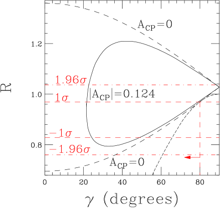
Figure 26: Behavior of R for $r=0.166$ and $|A_{\rm CP}|=0$ (dashed curve) or $|A_{\rm CP}|=0.124$ (solid curve), as a function of $\gamma$. The short-dashed curve shows the Fleischer-Mannel bound. Taken from reference [108].

This figure was drawn for a very specific value, $r=0.166$. For that value, and using the LP2003 $1\sigma$ bounds on $R$ and $|A_{\rm CP}|$, Gronau and Rosner find $49^{\circ}<\gamma<80^{\circ}$ [108].

The lower bound does not remain if one allows for lower values of $r$. Also, both bounds disappear if we take the $2\sigma$ ranges for $R$. But the most striking feature of FIG. 26 is yet a third one. The Gronau-Rosner method restricts the solutions to lie in the region within the solid curve $|A_{\rm CP}|=0.124$ and the dashed curve $|A_{\rm CP}|=0$. For the sake of argument, let us now take $r=0.166$ and the $1\sigma$ horizontal bounds on $R$ (dashed, red horizontal lines). Then, there is a very restricted allowed region in the $R-\gamma$ plane and we get the bound mentioned above: $49^{\circ}<\gamma<80^{\circ}$. But this still leaves a $31^{\circ}$ uncertainty on $\gamma$. How could we improve on this? The answer is surprising. Because the curves for $|A_{\rm CP}|=0.124$ and $|A_{\rm CP}|=0$ lie so close to each other in the region of interest, improving the precision on this (CP violating) measurement does not improve much the precision on (the CP violating phase) $\gamma$. In contrast, improving the precision on the (CP conserving) observable $R$ can improve considerably the precision on (the CP violating phase) $\gamma$, as one can see by imagining that the lower $1\sigma$ horizontal line moves up slightly.

Thus

• a more precise constraint on $r$ is required in order to assess the effectiveness of this method;

• a better measurement of $R$ is needed;

• and, surprisingly, an improvement on the precision of the measurement of the CP conserving observable $R$ will be much more effective in constraining the CP violating phase $\gamma$ than an improvement on the CP violating observable $A_{\rm CP}$.

The details of the $B\rightarrow K\pi$ analysis in general, and of FIG. 26 in particular, depend crucially on the exact values for the observed branching ratios and CP asymmetries, which are still in a state of flux. This is even more important for the assessment of electroweak penguins to be performed in the next subsection. Nevertheless, our interest here is on general methods and not on the precise numerics. The ideas presented here will remain on our collective toolbox, even if the specific examples themselves turn out to be numerically uninteresting.

7.4.3 Searching for enhanced $\Delta I=1$ contributions

The amplitudes discussed in the previous section may also be decomposed in terms of isospin amplitudes, according to [114] (Ex-32)

$$A(B^{0}_{d}\rightarrow K^{+}\pi^{-}) = -B_{1/2}+A_{1/2}+A_{3/2},$$

$$\sqrt{2}A(B^{+}\rightarrow K^{+}\pi^{0}) = -B_{1/2}-A_{1/2}+2A_{3/2},$$

$$A(B^{+}\rightarrow K^{0}\pi^{+}) = B_{1/2}+A_{1/2}+A_{3/2},$$

$$\sqrt{2}A(B^{0}\rightarrow K^{0}\pi^{0}) = B_{1/2}-A_{1/2}+2A_{3/2},$$ (283)

where $A$ and $B$ are $\Delta I=1$ and $\Delta I=0$ amplitudes, respectively, and the subscripts indicate the isospin of $K\pi$. Comparing Eq. (283) with FIG. 25 [115], we conclude that (Ex-33)

$$B_{1/2} = P+\frac{1}{2}T,$$

$$A_{1/2} = \frac{1}{3}P_{\rm EW}-\frac{1}{6}T,$$

$$A_{3/2} = -\frac{1}{3}P_{\rm EW}-\frac{1}{3}T.$$ (284)

Using both decompositions, one can show that (Ex-34)

$$R_{c}-R_{n}=\bigcirc\left(\frac{P_{\rm EW},T}{P}\right)^{2}\ \ \ \mbox{in a }\Delta I=1\mbox{ combination.}$$ (285)

Therefore, this observable highlights $\Delta I=1$ combinations which do not involve the gluonic penguin. In the SM, the right hand side of Eq. (285) is expected to be small. Hence, the fact that $R_{c}-R_{n}=0.42\pm 0.22$ in 2003 could be seen as an indication of new physics in electroweak penguins.

This question was first pointed out by Gronau and Rosner [115] and by Lipkin [116], utilizing a slightly different quantity (Ex-35)

$$R_{L}-1=2\frac{\Gamma_{\rm av}[B^{+}\rightarrow K^{+}\pi^{0}]+\Gamma_{\rm av}[B^{0}\rightarrow K^{0}\pi^{0}]}{\Gamma_{\rm av}[B^{+}\rightarrow K^{0}\pi^{+}]+\Gamma_{\rm av}[B^{0}\rightarrow K^{+}\pi^{-}]}-1=\frac{R_{c}+R/R_{n}}{1+R}-1,$$ (286)

which shares the features on the right hand side of Eq. (285) [117]. Averaging over CP conjugated decays is implicit in the notation $\Gamma_{\rm av}$ used on the first equality. It has been shown that it is possible to fit the LP2003 values for $R_{c}$ and $R_{n}$ as long as $P_{\rm EW}\sim iP/2$ [118]. Curiously, the search for new physics through such enhancements of $\Delta I=1$ electroweak penguins had been proposed sometime before, and those effects had been named “Trojan penguins” [119].

More recently, global analysis to all $B\rightarrow K\pi$ data were performed in [13] and [100], finding consistency with the SM and, in particular, uncovering no unequivocal sign of enhanced electroweak penguins. One could fear that, because these analysis involve a fit to many observables, most of which have nothing to do with possible enhanced $\Delta I=1$ pieces, some dilution might occur. However, the latest experimental results, presented at ICHEP2004, also seem to be moving in a way which removes this signal: $R_{c}-R_{n}=0.21\pm 0.16$ [104]. Whether this signal will remain is unclear, but even if it does not, we have learned of a new way to constrain theories with enhanced electroweak penguins.

7.4.4 CP asymmetries in $B\rightarrow K\pi$ decays

Perhaps the most important result in 2004 has been the improvement by BABAR [121] and Belle [122] of their measurements of the direct CP asymmetry in $B_{d}\rightarrow K^{\pm}\pi^{\mp}$. The average became $A_{\rm CP}(K^{+}\pi^{-})=-0.114\pm 0.020$ [103]. This constitutes the first observation of direct CP violation in the $B$ system agreed upon by both groups, in analogy to $\epsilon^{\prime}_{K}$ in the kaon system.

At ICHEP2004 a new puzzle emerged in $B\rightarrow K\pi$ decays, coming from

$$A_{\rm CP}(K^{+}\pi^{-})-A_{\rm CP}(K^{+}\pi^{0})=-0.163\pm 0.060\ ,$$ (287)

which constitutes a $3.6\sigma$ signal [103]. Looking back at FIG. 25, we recognize that this can only be due to electroweak penguins.

So, in 2004, the rave in $B\rightarrow K\pi$ decays moved from $R_{c}-R_{n}$ to the direct CP asymmetries. This is testimony to the fact that, after decades of experimental stagnation, CP violation has moved from theoretical exercises into a full fledged experimental endeavor. Since errors are still large, quite a number of additional interesting hints are to be expected.

7.5 Other decays of interest

In the coming years the programs developed at the $B$-factories and at hadronic facilities will greatly improve our knowledge of the CKM mechanism, and they hold the possibility to uncover new physics effects. It is impossible to mention all the decays of interest in a pedagogical review of this size. Some further possibilities for the $B_{d}$ system include:

• Snyder-Quinn method: determining $\beta+\gamma$ from the decays $B_{d}\rightarrow\rho\pi$ [123];

• Determining $\gamma$ from $B\rightarrow D$ decays. These ideas started with the Gronau-London-Wyler method, where one determines $\gamma$ through a triangle relation among the decays $B^{+}\rightarrow K^{+}D^{0}$, $B^{+}\rightarrow K^{+}\overline{D^{0}}$, $B^{+}\rightarrow K^{+}(f_{\rm cp})_{D}$ [124]. A very long list of improvements and related suggestions was spurred by the Atwood-Dunietz-Soni method [125].

• Determining $2\beta+\gamma$ from $B_{d}\rightarrow D$ decays. This interesting class of methods started with a proposal by Dunietz and Sachs and beats the phase of $B^{0}_{d}-\overline{B^{0}_{d}}$ mixing ($2\beta$ in the usual phase convention) against the phase in $b\rightarrow u$ transitions ($\gamma$ in the usual phase convention) [126].

Many interesting pieces of information will also come from experiments on the $B_{s}$ system performed at hadronic facilities. Indeed:

• A measurement of $\Delta m_{s}$ will reduce the hadronic uncertainties involved in extracting $|V_{td}|$ (i.e., $R_{t}=\sqrt{(1-\rho)^{2}+\eta^{2}}$) from $\Delta m_{d}$, thus improving our determination of $\rho$ and $\eta$;

• Since the angle $\chi$ is involved in $B^{0}_{s}-\overline{B^{0}_{s}}$ mixing (in the usual phase convention), it would be interesting to determine it, for example, from $B_{s}\rightarrow D_{s}^{+}D_{s}^{-}$ decays. Precisely because in the SM this asymmetry is expected to be small, this is a perfect channel to look for new physics;

• There are a variety of interesting CP asymmetries in $B_{s}$ decays. In the Aleksan-Dunietz-Kayser method one determines $\gamma$ through the decays $B_{s}\rightarrow D_{s}^{+}K^{-}$, $B_{s}\rightarrow D_{s}^{-}K^{+}$ [127];

• One may invoke SU(3) symmetry to compare $B_{d}$ and $B_{s}$ decays. For example, the Silva-Wolfenstein method utilizing $U$-spin to determine the penguin pollution in $B_{d}\rightarrow\pi^{+}\pi^{-}$ by its relation with $B_{d}\rightarrow K^{+}\pi^{-}$ [87] may be adapted to relate the penguin pollution in $B_{d}\rightarrow\pi^{+}\pi^{-}$ by its relation with $B_{s}\rightarrow K^{+}K^{-}$ instead [128].

This “Brave New World” will provide us with many new tests of the SM and, if we are lucky enough, the uncovering of new physics.

Appendix A Neutral meson mixing including CPT violation

A.1 The mixing matrix

In this appendix we discuss the mixing in the neutral meson systems in the presence of CPT violation and we will continue to assume the Lee-Oehme-Yang approximation [129]. The eigenvector equation (29) becomes generalized into

$$\left(\begin{array}[]{c}|P_{H}\rangle\\ |P_{L}\rangle\end{array}\right)=\left(\begin{array}[]{cc}p_{H}&-q_{H}\\ p_{L}&q_{L}\end{array}\right)\ \left(\begin{array}[]{c}|P^{0}\rangle\\ |\overline{P^{0}}\rangle\end{array}\right)=\mbox{\boldmath$X$}^{T}\ \left(\begin{array}[]{c}|P^{0}\rangle\\ |\overline{P^{0}}\rangle\end{array}\right).$$ (296)

We should be careful with the explicit choice of $-q_{H}$ and $+q_{L}$ in Eq. (296); the opposite choice has been made in references [1, 23].

The relation between these mixing parameters ($p_{H}$, $q_{H}$, $p_{L}$, and $q_{L}$), the eigenvalues of $H$ in Eq. (20), and the matrix elements of $H$ written in the flavor basis is still obtained through the diagonalization

$$\mbox{\boldmath$X$}^{-1}\mbox{\boldmath$H$}\mbox{\boldmath$X$}=\left(\begin{array}[]{cc}\mu_{H}&0\\ 0&\mu_{L}\end{array}\right),$$ (297)

but now

$$\mbox{\boldmath$X$}^{-1}=\frac{1}{p_{H}q_{L}+p_{L}q_{H}}\left(\begin{array}[]{cc}q_{L}&-p_{L}\\ q_{H}&p_{H}\end{array}\right)$$ (298)

substitutes Eq. (33).

We may write the mixing matrix $X$ in terms of new parameters [130]

$$\theta=\frac{\frac{q_{H}}{p_{H}}-\frac{q_{L}}{p_{L}}}{\frac{q_{H}}{p_{H}}+\frac{q_{L}}{p_{L}}},$$ (299)

and

$$\frac{q}{p}=-\sqrt{\frac{q_{H}q_{L}}{p_{H}p_{L}}}$$ (300)

We may define $\delta$ in this more general setting through the first equality in Eq. (39), leading to $|q/p|=\sqrt{\frac{1-\delta}{1+\delta}}$. With this notation the mixing matrix may be re-written as

$$\mbox{\boldmath$X$}=\left(\begin{array}[]{cc}1&1\\ -\frac{q}{p}\sqrt{\frac{1+\theta}{1-\theta}}&\frac{q}{p}\sqrt{\frac{1-\theta}{1+\theta}}\end{array}\right)\left(\begin{array}[]{cc}p_{H}&0\\ 0&p_{L}\end{array}\right),$$ (301)

$$\mbox{\boldmath$X$}^{-1}=\left(\begin{array}[]{cc}p_{H}^{-1}&0\\ 0&p_{L}^{-1}\end{array}\right)\left(\begin{array}[]{cc}\frac{1-\theta}{2}&-\frac{p}{q}\frac{\sqrt{1-\theta^{2}}}{2}\\ \frac{1+\theta}{2}&\frac{p}{q}\frac{\sqrt{1-\theta^{2}}}{2}\end{array}\right).$$ (302)

The fact that the trace and determinant are invariant under the general similarity transformation in Eq. (297) implies that

$$\mu = (H_{11}+H_{22})/2,$$

$$\Delta\mu = \sqrt{4H_{12}H_{21}+(H_{22}-H_{11})^{2}}.$$ (303)

Moreover, from

$$\left(\begin{array}[]{cc}H_{11}&H_{12}\\ H_{21}&H_{22}\end{array}\right)\left(\begin{array}[]{c}p_{H}\\ -q_{H}\end{array}\right) = \mu_{H}\left(\begin{array}[]{c}p_{H}\\ -q_{H}\end{array}\right),$$ (310)

$$\left(\begin{array}[]{cc}H_{11}&H_{12}\\ H_{21}&H_{22}\end{array}\right)\left(\begin{array}[]{c}p_{L}\\ q_{L}\end{array}\right) = \mu_{L}\left(\begin{array}[]{c}p_{L}\\ q_{L}\end{array}\right).$$ (317)

we find that

$$\frac{q_{H}}{p_{H}} = \frac{H_{11}-\mu_{H}}{H_{12}}=\frac{H_{21}}{H_{22}-\mu_{H}},$$

$$\frac{q_{L}}{p_{L}} = \frac{\mu_{b}-H_{11}}{H_{12}}=\frac{H_{21}}{\mu_{b}-H_{22}},$$ (318)

leading to

$$\theta = \frac{H_{22}-H_{11}}{\mu_{H}-\mu_{L}},$$

$$\delta = \frac{|H_{12}|-|H_{21}|}{|H_{12}|+|H_{21}|},$$ (319)

and $q/p=-\sqrt{H_{21}/H_{12}}$. We see from Eqs. (18) that $\mbox{Re}\,\theta$ and $\mbox{Im}\,\theta$ are CP and CPT violating, while $\delta$ is CP and T violating.

Although $H$ contains eight real numbers, only seven are physically meaningful. Indeed, one is free to change the phase of the kets $|P^{0}\rangle$, $|\overline{P^{0}}\rangle$, $|P_{H}\rangle$, and $|P_{L}\rangle$, as

$$|P^{0}\rangle \rightarrow e^{i\gamma}|P^{0}\rangle,$$

$$|\overline{P^{0}}\rangle \rightarrow e^{i\overline{\gamma}}|\overline{P^{0}}\rangle,$$

$$|P_{H}\rangle \rightarrow e^{i\gamma_{H}}|P_{H}\rangle,$$

$$|P_{L}\rangle \rightarrow e^{i\gamma_{L}}|P_{L}\rangle.$$ (320)

Under these transformations

$$H_{12} \rightarrow e^{i\left(\overline{\gamma}-\gamma\right)}H_{12},$$

$$H_{21} \rightarrow e^{i\left(\gamma-\overline{\gamma}\right)}H_{21},$$

$$q/p \rightarrow e^{i\left(\gamma-\overline{\gamma}\right)}q/p,$$ (321)

while $H_{11}$, $H_{22}$, $\mu$, $\Delta\mu$, $\theta$, and $\delta$ do not change. Therefore, the relative phase between $H_{12}$ and $H_{21}$ is physically meaningless and $H$ contains only seven observables. Similarly, the phase of $q/p$ is also unphysical. As a result, we have four observables in the eigenvalues, $\mu$ and $\Delta\mu$, and three in the mixing matrix, $\theta$ and $\delta$ (or, alternatively, $|q/p|$).

Eqs. (303) and (319) give the measurable mixing and eigenvalue parameters in terms of the $H_{ij}$ matrix elements which one can calculate in a given model. Given the current and upcoming experimental probes of the various neutral meson systems, it seems much more appropriate to do precisely the opposite; that is, to give the $H_{ij}$ matrix elements in terms of the experimentally accessible quantities. Such expressions would give $M_{ij}$ and $\Gamma_{ij}$ in a completely model independent way, with absolutely no assumptions. One could then calculate these quantities in any given model; if they fit in the allowed ranges the model would be viable.

Surprisingly, this is not is done in most expositions of the $P^{0}-\overline{P^{0}}$ mixing. The reason is simple. Eqs. (303) and (319) are non-linear in the $H_{ij}$ matrix elements. Thus, inverting them by brute force would entail a tedious calculation. With the matrix manipulation discussed here this inversion is straightforward. Indeed, Eq. (297) can be trivially transformed into [33, 23]

$$H = \mbox{\boldmath$X$}\left(\begin{array}[]{cc}\mu_{H}&0\\ 0&\mu_{L}\end{array}\right)\mbox{\boldmath$X$}^{-1}$$ (324)

$$= \left(\begin{array}[]{cc}\mu-\frac{\Delta\mu}{2}\theta&-\frac{p}{q}\frac{\sqrt{1-\theta^{2}}}{2}\Delta\mu\\[5.69054pt] -\frac{q}{p}\frac{\sqrt{1-\theta^{2}}}{2}\Delta\mu&\mu+\frac{\Delta\mu}{2}\theta\end{array}\right),$$ (327)

where we have used Eqs. (301) and (302) (Ex-36). Although rarely seen, this equation is very interesting because it expresses in a very compact form the relation between the quantities which are experimentally accessible and those which are easily calculated in a given theory. The full power of Eq. (327) can be seen when considering the propagation of a neutral meson system in matter (Ex-37).

A.2 Time evolution

To find the time evolution of the neutral meson system we start from Eq. (365) proved as an exercise. Then, using Eqs. (61), (296), (301), and (302), we find

$$\exp{(-i{\cal H}t)} = \left(\begin{array}[]{cc}|P^{0}\rangle,&|\overline{P^{0}}\rangle\end{array}\right)\mbox{\boldmath$X$}\left(\begin{array}[]{cc}e^{-i\mu_{H}t}&0\\ 0&e^{-i\mu_{L}t}\end{array}\right)\mbox{\boldmath$X$}^{-1}\left(\begin{array}[]{c}\langle P^{0}|\\ \langle\overline{P^{0}}|\end{array}\right)$$ (333)

$$= \left(\begin{array}[]{cc}|P^{0}\rangle,&|\overline{P^{0}}\rangle\end{array}\right)\left(\begin{array}[]{cc}g_{+}(t)+\theta\,g_{-}(t)&\frac{p}{q}\sqrt{1-\theta^{2}}g_{-}(t)\\[5.69054pt] \frac{q}{p}\sqrt{1-\theta^{2}}g_{-}(t)&g_{+}(t)-\theta\,g_{-}(t)\end{array}\right)\left(\begin{array}[]{c}\langle P^{0}|\\ \langle\overline{P^{0}}|\end{array}\right),$$ (339)

where the functions $g_{\pm}(t)$ are those already defined in Eq. (68). This corresponds to the usual expressions for the time evolution of a state which starts out as $P^{0}$ or $\overline{P^{0}}$,

$$|P^{0}(t)\rangle=\exp{(-i{\cal H}t)}|P^{0}\rangle = \left[g_{+}(t)+\theta\,g_{-}(t)\right]|P^{0}\rangle+\frac{q}{p}\sqrt{1-\theta^{2}}g_{-}(t)\,|\overline{P^{0}}\rangle,$$

$$|\overline{P^{0}}(t)\rangle=\exp{(-i{\cal H}t)}|\overline{P^{0}}\rangle = \frac{p}{q}\sqrt{1-\theta^{2}}g_{-}(t)|P^{0}\rangle+\left[g_{+}(t)-\theta\,g_{-}(t)\right]|\overline{P^{0}}\rangle,$$ (340)

respectively. At this point it is important to emphasize the fact that, in deriving this result, no assumptions were made about the form of the original matrix $H$. This observation will become important once we consider the evolution in matter (Ex-37).

Appendix B Phase transformations and CP conservation

This appendix contains a detailed description of the phase transformations and of the conditions implied by CP conservation which we have used in chapter 4 in order to identify the relevant CP violating parameters.

B.1 Phase transformations

As mentioned, any “ket” may be redefined by an arbitrary phase transformation [16],

$$|i\rangle\rightarrow e^{i\gamma_{i}}|i\rangle\ , |\bar{i}\rangle\rightarrow e^{i\overline{\gamma}_{i}}|\bar{i}\rangle\ ,$$

$$|P^{0}\rangle\rightarrow e^{i\gamma_{P}}|P^{0}\rangle\ , |\overline{P^{0}}\rangle\rightarrow e^{i\overline{\gamma}_{P}}|\overline{P^{0}}\rangle\ ,$$

$$|f\rangle\rightarrow e^{i\gamma_{f}}|f\rangle\ , |\bar{f}\rangle\rightarrow e^{i\overline{\gamma}_{f}}|\bar{f}\rangle\ .$$ (341)

These phase transformations modify the mixing parameters and the transition amplitudes, according to

$$\frac{q}{p}\rightarrow e^{i(\gamma_{P}-\overline{\gamma}_{P})}\frac{q}{p}\ ,$$

$$A_{i\rightarrow P^{0}}\rightarrow e^{i(\gamma_{i}-\gamma_{P})}A_{i\rightarrow P^{0}}\ , A_{\bar{i}\rightarrow P^{0}}\rightarrow e^{i(\overline{\gamma}_{i}-\gamma_{P})}A_{\bar{i}\rightarrow P^{0}}\ ,$$

$$A_{i\rightarrow\overline{P^{0}}}\rightarrow e^{i(\gamma_{i}-\overline{\gamma}_{P})}A_{i\rightarrow\overline{P^{0}}}\ , A_{\bar{i}\rightarrow\overline{P^{0}}}\rightarrow e^{i(\overline{\gamma}_{i}-\overline{\gamma}_{P})}A_{\bar{i}\rightarrow\overline{P^{0}}}\ ,$$

$$A_{f}\rightarrow e^{i(\gamma_{P}-\gamma_{f})}A_{f}\ , \bar{A}_{f}\rightarrow e^{i(\overline{\gamma}_{P}-\gamma_{f})}\bar{A}_{f}\ ,$$

$$A_{\bar{f}}\rightarrow e^{i(\gamma_{P}-\overline{\gamma}_{f})}A_{\bar{f}}\ , \bar{A}_{\bar{f}}\rightarrow e^{i(\overline{\gamma}_{P}-\overline{\gamma}_{f})}\bar{A}_{\bar{f}}\ .$$ (342)

Only those quantities which remain invariant under these redefinitions may have physical meaning. Clearly, the magnitudes of all the quantities in Eq. (B.1) satisfy this criterion.

Besides these, there are quantities which remain invariant under phase redefinitions and which arise from the “interference” between the parameters describing the mixing and those describing the transitions:

$$\lambda_{f}\equiv\frac{q}{p}\frac{\bar{A}_{f}}{A_{f}}\ , \lambda_{\bar{f}}\equiv\frac{q}{p}\frac{\bar{A}_{\bar{f}}}{A_{\bar{f}}}\ ,$$ (343)

$$\xi_{i\rightarrow P}\equiv\frac{A_{i\rightarrow\overline{P^{0}}}}{A_{i\rightarrow P^{0}}}\frac{p}{q}\ , \xi_{\bar{i}\rightarrow P}\equiv\frac{A_{\bar{i}\rightarrow\overline{P^{0}}}}{A_{\bar{i}\rightarrow P^{0}}}\frac{p}{q}\ .$$ (344)

The parameters in Eq. (343) describe the interference between between mixing in the neutral meson system and its subsequent decay into the final states $f$ and $\bar{f}$. In contrast, the parameters in Eq. (344) describe the interference between the production of the neutral meson system and the mixing in that system.

B.2 Conditions for CP conservation

If CP were conserved, then there would exist phases $\xi_{i}$, $\xi$ and $\xi_{f}$, as well as a CP eigenvalue, $\eta_{P}=\pm 1$, such that

$${\cal CP}|i\rangle = e^{i\xi_{i}}|\bar{i}\rangle\ ,$$

$${\cal CP}|P^{0}\rangle = e^{i\xi}|\overline{P^{0}}\rangle\ ,$$

$${\cal CP}|f\rangle = e^{i\xi_{f}}|\bar{f}\rangle\ ,$$ (345)

and

$${\cal CP}|P_{H}\rangle = \eta_{P}|P_{H}\rangle\ ,$$

$${\cal CP}|P_{L}\rangle = -\eta_{P}|P_{L}\rangle\ ,$$ (346)

where, as usual $H$ ($L$) refers to the “heavy” (“light”) eigenvalue. Here, we use the convention $\Delta m>0$. With this convention, it is the sign of $\eta_{P}$ which must be determined by experiment. For example, we know from experiment that the heavier kaon also has the longest lifetime. Moreover, if there were no CP violation in the mixture of neutral kaons, this state would be CP odd. As a result, we must use $\eta_{K}=-1$ whenever we neglect the mixing in the neutral kaon system.

On the other hand, the CP transformation of the multi-particle intermediate state $XP$ is given by

$${\cal CP}|XP^{0}\rangle=\eta_{X}e^{i\xi}|\overline{X}\,\overline{P^{0}}\rangle\ .$$ (347)

Here, $\eta_{X}$ contains the CP transformation properties of the state $X$, as well as the parity properties corresponding to the relative orbital angular momentum between $X$ and $P$.

From Eqs. (345), (346), and (347), we derive the conditions required for CP invariance,

$$\frac{q}{p}=-\eta_{P}e^{i\xi}$$ (348)

and

$$A_{i\rightarrow P^{0}}=\eta_{X}e^{i(\xi_{i}-\xi)}A_{\bar{i}\rightarrow\overline{P^{0}}}\ , A_{i\rightarrow\overline{P^{0}}}=\eta_{X}e^{i(\xi_{i}+\xi)}A_{\bar{i}\rightarrow P^{0}}\ ,$$

$$A_{f}=e^{i(\xi-\xi_{f})}\bar{A}_{\bar{f}}\ , A_{\bar{f}}=e^{i(\xi+\xi_{f})}\bar{A}_{f}\ .$$ (349)

Therefore, if CP were a good symmetry we would have

$$\left|\frac{q}{p}\right|=1\ ,$$

$$\left|A_{i\rightarrow P^{0}}\right|=\left|A_{\bar{i}\rightarrow\overline{P^{0}}}\right|\ , \left|A_{i\rightarrow\overline{P^{0}}}\right|=\left|A_{\bar{i}\rightarrow P^{0}}\right|\ ,$$

$$\left|A_{f}\right|=\left|\bar{A}_{\bar{f}}\right|\ , \left|A_{\bar{f}}\right|=\left|\bar{A}_{f}\right|\ .$$ (350)

Also, the parameters describing interference CP violation would become related by

$$\lambda_{f}\,\lambda_{\bar{f}} = 1\ ,$$

$$\xi_{i\rightarrow P}\,\xi_{\bar{i}\rightarrow P} = 1\ .$$ (351)

This means that, if CP were conserved, then $\arg\lambda_{f}+\arg\lambda_{\bar{f}}$ and $\arg\xi_{i\rightarrow P}+\arg\xi_{\bar{i}\rightarrow P}$ would vanish. We may use Eqs. (348) and (349) in order to find more complicated conditions for CP invariance, such as

$$A_{\bar{i}\rightarrow\overline{P^{0}}}\bar{A}_{f}(A_{\bar{i}\rightarrow P^{0}})^{\ast}(A_{f})^{\ast}=A_{i\rightarrow P^{0}}A_{\bar{f}}(A_{i\rightarrow\overline{P^{0}}})^{\ast}(\bar{A}_{\bar{f}})^{\ast}.$$ (352)

A very important particular case occurs when the final state $f$ is an eigenstate of CP. In that case, $\eta_{f}\equiv e^{i\xi_{f}}=\pm 1$, and the conditions for CP invariance become

$$\left|A_{f}\right|=\left|\bar{A}_{f}\right|\ \ \mbox{e }\ \ \lambda_{f}=\eta_{P}\eta_{f}.$$ (353)

As mentioned in the main text, we have just found the usual three types of CP violation

1. $|q/p|-1$ describes CP violation in the mixing of the neutral meson system;

2. $|A_{i\rightarrow P^{0}}|-|A_{\bar{i}\rightarrow\overline{P^{0}}}|$ and $|A_{i\rightarrow\overline{P^{0}}}|-|A_{\bar{i}\rightarrow P^{0}}|$, on the one hand, and $|A_{f}|-|\bar{A}_{\bar{f}}|$ and $|A_{\bar{f}}|-|\bar{A}_{f}|$, on the other hand, describe the CP violation present directly in the production of the neutral meson system and in its decay, respectively;

3. $\arg\lambda_{f}+\arg\lambda_{\bar{f}}$ measures the CP violation arising from the interference between mixing in the neutral meson system and its subsequent decay into the final states $f$ and $\bar{f}$. We call this the “interference CP violation: first mix, then decay”. When $f=f_{cp}$ is an CP eigenstate, this CP violating observable $\arg\lambda_{f}+\arg\lambda_{\bar{f}}$, becomes proportional to $\mbox{Im}\lambda_{f}$.

However, we can also identify a new type of CP violating observable

$$\arg\xi_{i\rightarrow P}+\arg\xi_{\bar{i}\rightarrow P}.$$ (354)

This observable measures the CP violation arising from the interference between the production of the neutral meson system and the mixing in that system. We call this the “interference CP violation: first produce, then mix”.

Appendix C Exercises

• Prove Eqs. (3). For one single pion, ${\cal CP}\pi^{\pm}=-\pi^{\mp}$, ${\cal CP}\pi^{0}=-\pi^{0}$. You should check in an introductory book that these properties may be inferred, for example, from the processes $\pi^{-}+d\rightarrow n+n$ and $\pi^{0}\rightarrow\gamma\gamma$, and require an implicit phase convention (see, for example, reference [1]). For multiple pions we must worry about the relative angular momentum, since the orbital wave functions change with P as $(-1)^{L}$. Clearly, the system of two pions originating from a kaon decay must be in a relative S wave.

• Using Eqs. (29) and (33), check that $\mbox{\boldmath$X$}\mbox{\boldmath$X$}^{-1}=\mbox{\boldmath$X$}^{-1}\mbox{\boldmath$X$}=\mbox{\boldmath$1$}$.

• Prove the last equality of Eq. (37).

• Using Eqs. (3.2)–(39), show that

  $$|M_{12}|^{2} = \frac{4(\Delta m)^{2}+\delta^{2}(\Delta\Gamma)^{2}}{16(1-\delta^{2})},$$

  $$|\Gamma_{12}|^{2} = \frac{(\Delta\Gamma)^{2}+4\delta^{2}(\Delta m)^{2}}{4(1-\delta^{2})},$$ (355)

  and

  $$(\Delta m)^{2} = \frac{4|M_{12}|^{2}-\delta^{2}|\Gamma_{12}|^{2}}{1+\delta^{2}},$$

  $$(\Delta\Gamma)^{2} = \frac{4|\Gamma_{12}|^{2}-16\delta^{2}|M_{12}|^{2}}{1+\delta^{2}}.$$ (356)

  Show also that

  $$-\frac{q}{p}\Gamma_{12} = \frac{y+i\delta x}{1+\delta}\Gamma,$$

  $$-\frac{q}{p}M_{12} = \frac{x-i\delta y}{2(1+\delta)}\Gamma,$$ (357)

  where $x$ and $y$ are defined in Eq. (82).

• To reach this conclusion in a different way, use Eq. (37) to prove that

  $$\left[\mbox{\boldmath$H$},\mbox{\boldmath$H$}^{\dagger}\right]=\left|\Delta\mu\right|^{2}\frac{\delta}{1-\delta^{2}}\left(\begin{array}[]{cc}1&0\\ 0&-1\end{array}\right),$$ (358)

  meaning that this commutator is directly proportional to the CP violating observable $\delta$. If you need to use

  $$\left|\frac{q}{p}\right|^{2}=\frac{1-\delta}{1+\delta},$$ (359)

  prove it first.

• Here you prove Eqs. (68)–(69) fully in matrix form, starting from Eq. (59). Use Eqs. (62) and (63), together with the fact that $|P_{H}\rangle\langle\tilde{P}_{H}|$ and $|P_{L}\rangle\langle\tilde{P}_{L}|$ are projection operators, in order to show that

  $$\exp{(-i{\cal H}t)} = e^{-i\mu_{H}t}|P_{H}\rangle\langle\tilde{P}_{H}|+e^{-i\mu_{L}t}|P_{L}\rangle\langle\tilde{P}_{L}|.$$ (365)

  $$= \left(\begin{array}[]{cc}|P_{H}\rangle,&|P_{L}\rangle\end{array}\right)\left(\begin{array}[]{cc}e^{-i\mu_{H}t}&0\\ 0&e^{-i\mu_{L}t}\end{array}\right)\left(\begin{array}[]{c}\langle\tilde{P}_{H}|\\ \langle\tilde{P}_{L}|\end{array}\right).$$

  In fact, so far you have just taken a rather long path to prove the trivial statements in Eqs. (64). Now, use Eqs. (29), (33), and (61), to show that

  $$\exp{(-i{\cal H}t)} = \left(\begin{array}[]{cc}|P^{0}\rangle,&|\overline{P^{0}}\rangle\end{array}\right)\mbox{\boldmath$X$}\left(\begin{array}[]{cc}e^{-i\mu_{H}t}&0\\ 0&e^{-i\mu_{L}t}\end{array}\right)\mbox{\boldmath$X$}^{-1}\left(\begin{array}[]{c}\langle P^{0}|\\ \langle\overline{P^{0}}|\end{array}\right)$$ (371)

  $$= \left(\begin{array}[]{cc}|P^{0}\rangle,&|\overline{P^{0}}\rangle\end{array}\right)\left(\begin{array}[]{cc}g_{+}(t)&\frac{p}{q}g_{-}(t)\\[5.69054pt] \frac{q}{p}g_{-}(t)&g_{+}(t)\end{array}\right)\left(\begin{array}[]{c}\langle P^{0}|\\ \langle\overline{P^{0}}|\end{array}\right).$$ (377)

  Get Eq. (69) from this.

• Prove Eqs. (80).

• Check Eqs. (81)–(82).

• Prove all the equalities in Eq. (85).

• Prove Eqs. (91)–(94).

• Prove Eqs. (95) and (96).

• To practice with this compact notation, write the $h.c.$ (hermitian conjugated) terms of Eq. (110) explicitly. Clearly, the final expression is a number, and one may decide to rewrite the expression by taking its transpose. If one does this, one must include an explicit minus sign, which arises from the fact that, when taking the transpose, one is interchanging the position of two fermion fields which, as such, anti-commute. This detail will be important for (Ex-16, Ex-17, Ex-20).

• Defining

  $$W_{\mu}^{\pm} = \frac{W_{\mu}^{1}\mp iW_{\mu}^{2}}{\sqrt{2}},$$

  $$\tau_{\pm} = \frac{\tau_{1}\pm i\tau_{2}}{\sqrt{2}},$$

  $$e = g\sin{\theta_{W}}=g^{\prime}\cos{\theta_{W}},$$ (378)

  and

  $$Q=\frac{1}{2}\tau_{3}+Y,$$ (379)

  show that

  $$-\frac{g}{2}\,\vec{\tau}.\vec{W}_{\mu}-g^{\prime}\,YB_{\mu}=$$

  $$\hskip 19.91692pt-\frac{g}{2}\left(\tau_{+}W_{\mu}^{+}+\tau_{-}W_{\mu}^{-}\right)-eQA_{\mu}-\frac{g}{\cos{\theta_{W}}}\left(\frac{1}{2}\tau_{3}-Q\sin^{2}{\theta_{W}}\right)Z_{\mu}.$$ (380)

  Use this to prove that Eqs. (115) and (116) follow from Eqs. (108) and (109).

• Show that Eq. (127) follows from Eqs. (110) and (113), with the basis transformations in Eqs. (125).

• Show that Eqs. (128)–(129) follow by applying the basis transformations in Eqs. (125) to Eqs. (115)–(116).

• Recalling that $\gamma^{0}\gamma^{\mu}\gamma^{0}=\gamma_{\mu}$, $C^{-1}\gamma_{\mu}C=-\gamma_{\mu}^{T}$, and the other trivialities about Dirac $\gamma$-matrices, use the CP transformations in Eq. (137), to prove that:

  $$\left({\cal CP}\right)\bar{u}d\left({\cal CP}\right)^{\dagger} = e^{i(\xi_{d}-\xi_{u})}\,\bar{d}u,$$

  $$\left({\cal CP}\right)\bar{u}\gamma_{5}d\left({\cal CP}\right)^{\dagger} = -e^{i(\xi_{d}-\xi_{u})}\,\bar{d}\gamma_{5}u,$$

  $$\left({\cal CP}\right)\bar{u}\gamma^{\mu}d\left({\cal CP}\right)^{\dagger} = -e^{i(\xi_{d}-\xi_{u})}\,\bar{d}\gamma_{\mu}u,$$

  $$\left({\cal CP}\right)\bar{u}\gamma^{\mu}\gamma_{5}d\left({\cal CP}\right)^{\dagger} = -e^{i(\xi_{d}-\xi_{u})}\,\bar{d}\gamma_{\mu}\gamma_{5}u,$$ (381)

  where an extra minus sign appears when taking the transpose, because the two fermion fields anti-commute. Also,

  $$\left({\cal CP}\right)\left[\bar{u}\gamma^{\mu}(1-\gamma_{5})d\right]\left({\cal CP}\right)^{\dagger}=-e^{i(\xi_{d}-\xi_{u})}\left[\bar{d}\gamma_{\mu}(1-\gamma_{5})u\right].$$ (382)

• Verify that the Lagrangian in Eq. (138) is invariant under the CP transformations in Eq. (137) if and only if Eq. (139) holds.

• Define

  $$Q_{\alpha i\beta j}=V_{\alpha i}V_{\beta j}V_{\alpha j}^{\ast}V_{\beta i}^{\ast},$$ (383)

  and show that $Q_{\alpha i\beta j}=Q_{\beta j\alpha i}=Q_{\alpha j\beta i}^{\ast}=Q_{\beta i\alpha j}^{\ast}$. Thus, $\mbox{Im}Q_{\alpha i\beta j}$ may change sign under a reshuffling of the indexes, and the magnitude is useful in Eq. (141).

• Prove that [11]

  $$\mbox{Im}\left(V_{\alpha i}V_{\beta j}V_{\alpha j}^{\ast}V_{\beta i}^{\ast}\right)=J_{\rm CKM}\sum_{\gamma=1}^{3}\sum_{k=1}^{3}\epsilon_{\alpha\beta\gamma}\epsilon_{ijk}.$$ (384)

• Verify that the Yukawa Lagrangian in Eq. (110) is invariant under the CP transformations in Eq. (143) if and only if Eq. (144) holds.

• Show that

  $$\mbox{Im}\left\{\mbox{Tr}\left(H_{u}H_{d}\right)\right\}=0=\mbox{Im}\left\{\mbox{Tr}\left(H_{u}^{2}H_{d}^{2}\right)\right\}.$$ (385)

• Show that

  $$\mbox{Im}\left\{\mbox{Tr}\left(H_{u}H_{d}H_{u}^{2}H_{d}^{2}\right)\right\}=\sum_{\alpha,\beta=u,c,t}\,\sum_{i,j=d,s,b}m_{u_{\alpha}}^{2}m_{d_{i}}^{2}m_{u_{\beta}}^{4}m_{d_{j}}^{4}\mbox{Im}\left(Q_{\alpha i\beta j}\right)$$

  $$=(m_{t}^{2}-m_{c}^{2})(m_{t}^{2}-m_{u}^{2})(m_{c}^{2}-m_{t}^{2})(m_{b}^{2}-m_{s}^{2})(m_{b}^{2}-m_{d}^{2})(m_{s}^{2}-m_{d}^{2})J_{\rm CKM}.$$ (386)

  You may need the result in (Ex-19).

• Show that the Chau–Keung parametrization in Eq. (149) results from

  $$V=\left(\begin{array}[]{ccc}1&0&0\\ 0&c_{23}&s_{23}\\ 0&-s_{23}&c_{23}\end{array}\right)\,\left(\begin{array}[]{ccc}c_{13}&0&s_{13}e^{-i\delta_{13}}\\ 0&1&0\\ -s_{13}e^{i\delta_{13}}&0&c_{13}\end{array}\right)\,\left(\begin{array}[]{ccc}c_{12}&s_{12}&0\\ -s_{12}&c_{12}&0\\ 0&0&1\end{array}\right).$$ (387)

• Prove that the definitions of $\alpha$, $\beta$, and $\gamma$ in Eqs. (158)–(160) imply that $\alpha+\beta+\gamma=\mbox{arg}(-1)$, leading to Eq. (162).

• Use the unitarity of the CKM matrix in order to prove Eqs. (163).

• Prove that all the triangles in Eqs. (170)–(175) have the same area $J_{\rm CKM}/2$.

• Obtain Eq. (176) from Eq. (172) and the definitions in Eqs. (156)–(160). Use the Wolfenstein parametrization, through Eqs. (164) and (165) to show that this represents a triangle which has an apex at coordinates $(\rho,\eta)$ and area $|\eta|/2$. Check also how much simpler this gets if one uses instead the redundant parametrization in Eq. (169).

• Expand Eq. (204) to first order in $r$. Substituting into Eqs. (93) and (94), verify Eqs. (208) and (209).

• The diagram in FIG. 9 is proportional to $V_{cb}^{\ast}V_{cs}\sim(A\lambda^{2})(1)$ and, thus, it carries no weak phase in the standard phase convention for the CKM matrix. Use this, together with Eqs. (220) and (221), to show that

  $$\lambda_{B_{d}\rightarrow J/\psi K_{S}}=-e^{-2i(\tilde{\beta}-\chi^{\prime})}.$$ (388)

  In the absence of new physics in $B^{0}_{d}-\overline{B^{0}_{d}}$ mixing, $\tilde{\beta}=\beta$, and we recover the result on the last line of Eq. (219). Now we know why most people ignore the spurious phases $\xi$.

• Here we study the isospin decomposition of the decay amplitudes for $B\rightarrow\pi\pi$ in some detail.

  • Since the pions are spinless, they must arise from $B$ decays in an $s$ wave and they must be in an overall symmetric state. This implies a symmetric isospin configuration. Use addition of angular momenta to show that the resulting final states are:

    $$\langle\pi^{0}\pi^{0}| = \sqrt{\frac{2}{3}}\langle 2,0|-\sqrt{\frac{1}{3}}\langle 0,0|,$$

    $$\langle\pi^{+}\pi^{-}| \equiv \frac{1}{\sqrt{2}}\left(\langle\pi_{1}^{+}\pi_{2}^{-}|+\langle\pi_{1}^{-}\pi_{2}^{+}|\right)=\sqrt{\frac{1}{3}}\langle 2,0|+\sqrt{\frac{2}{3}}\langle 0,0|,$$

    $$\langle\pi^{+}\pi^{0}| \equiv \frac{1}{\sqrt{2}}\left(\langle\pi_{1}^{+}\pi_{2}^{0}|+\langle\pi_{1}^{0}\pi_{2}^{+}|\right)=\langle 2,1|.$$ (389)

  • The first two channels are reached by $|B^{0}_{d}\rangle=|1/2,-1/2\rangle$, the third by $|B^{+}\rangle=|1/2,1/2\rangle$. In general, the transition matrix has $\Delta I=1/2$, $\Delta I=3/2$, and $\Delta I=5/2$ pieces. Use the Wigner-Eckart theorem to show that

    $$\langle\pi^{0}\pi^{0}|T|B^{0}_{d}\rangle = -\sqrt{\frac{1}{3}}A_{1/2}+\sqrt{\frac{1}{6}}A_{3/2}-\sqrt{\frac{1}{6}}A_{5/2},$$

    $$\langle\pi^{+}\pi^{-}|T|B^{0}_{d}\rangle = \sqrt{\frac{1}{6}}A_{1/2}+\sqrt{\frac{1}{3}}A_{3/2}-\sqrt{\frac{1}{3}}A_{5/2},$$

    $$\langle\pi^{+}\pi^{0}|T|B^{+}\rangle = \frac{\sqrt{3}}{2}A_{3/2}+\sqrt{\frac{1}{3}}A_{5/2},$$ (390)

    where $A_{k}$ are the relevant reduces matrix elements.

  • In the SM,

    • tree level diagrams — contribute to $A_{1/2}$ and $A_{3/2}$;

    • gluonic penguin diagrams — contribute only to $A_{1/2}$;

    • electroweak penguin diagrams — are expected to be small;

    • $A_{5/2}\sim\alpha A_{1/2}$ — arise from $A_{1/2}$ together with the $\Delta I=2$ electromagnetic rescattering of the two pions in the final state [133]. Because of the $\Delta I=1/2$ rule in place for the decay $K\rightarrow\pi\pi$, the contribution from $A_{5/2}$ is detectable and has been measured in the kaon system [134], but it is expected to be negligible in $B\rightarrow\pi\pi$ decays.

    Neglecting $A_{5/2}$, use Eqs. (390) to prove Eq. (244).

• Do the trivial exercise to get Eq. (281).

• Derive the isospin decomposition in Eq. (283).

• Check that Eq. (284) follows trivially by comparing Eq. (283) with FIG. 25. See [115] for a generalization, including other diagrams neglected here.

• Use the diagrammatic decomposition in FIG. 25 to show the first equality of Eq. (285). Use the isospin decomposition of Eq. (283) to show that the leading terms in $R_{c}-R_{n}$ are proportional to a quadratic combination of $A_{1/2}$ and $A_{3/2}$ over the square of $B_{1/2}$, thus explaining the written comment in Eq. (283).

• Prove the last equality in Eq. (286).

• Prove the last equality in Eq. (327) of appendix A.

• When a neutral meson system propagates through matter, it is subject to additional strangeness-preserving interactions which may be parametrized by

  $$\mbox{\boldmath$H$}_{\rm nuc}=\left(\begin{array}[]{cc}\chi&0\\ 0&\bar{\chi}\end{array}\right),$$ (391)

  which are written in the $P^{0}-\overline{P^{0}}$ rest frame and must be added to the Hamiltonian in vacuum. The full Hamiltonian in matter becomes

  $$\mbox{\boldmath$H$}^{\prime}=\mbox{\boldmath$H$}+\mbox{\boldmath$H$}_{\rm nuc},$$ (392)

  where we denote matrices, matrix elements and eigenvalues in vacuum by unprimed quantities and their analogues in matter by primed quantities.

  Now, we have already studied the most general effective Hamiltonian, and Eq. (327) relates such an Hamiltonian written in the flavor basis with the corresponding eigenvalues and mixing parameters. Use Eqs. (327), (391) and (392) to show that [23]

  $$\left(\begin{array}[]{cc}\mu^{\prime}-\frac{\Delta\mu^{\prime}}{2}\theta^{\prime}&-\frac{p^{\prime}}{q^{\prime}}\frac{\sqrt{1-\theta^{\prime 2}}}{2}\Delta\mu^{\prime}\\[5.69054pt] -\frac{q^{\prime}}{p^{\prime}}\frac{\sqrt{1-\theta^{\prime 2}}}{2}\Delta\mu^{\prime}&\mu^{\prime}+\frac{\Delta\mu^{\prime}}{2}\theta^{\prime}\end{array}\right)=\left(\begin{array}[]{cc}\mu-\frac{\Delta\mu}{2}\theta&-\frac{p}{q}\frac{\sqrt{1-\theta^{2}}}{2}\Delta\mu\\[5.69054pt] -\frac{q}{p}\frac{\sqrt{1-\theta^{2}}}{2}\Delta\mu&\mu+\frac{\Delta\mu}{2}\theta\end{array}\right)+\left(\begin{array}[]{cc}\chi&0\\ 0&\bar{\chi}\end{array}\right).$$ (393)

  Now prove the following results:

  • Clearly, $H^{\prime}_{12}=H_{12}$, $H^{\prime}_{21}=H_{21}$, and $q^{\prime}/p^{\prime}=q/p$. This means that the CP and T violating parameter $\delta$, which depends on $|q^{\prime}/p^{\prime}|=|q/p|$, is the same in vacuum and in the presence of matter.

  • Prove that the parameters in vacuum and in matter are related through,

    $$\mu^{\prime} = \mu+\frac{\chi+\bar{\chi}}{2},$$

    $$\Delta\mu^{\prime} = \sqrt{(\Delta\mu)^{2}+2\theta\,\Delta\mu\,\Delta\chi+(\Delta\chi)^{2}}=\Delta\mu\,\sqrt{1+4r\,\theta+4r^{2}},$$

    $$\theta^{\prime} = \frac{\Delta\mu\,\theta+\Delta\chi}{\sqrt{(\Delta\mu)^{2}+2\theta\,\Delta\mu\,\Delta\chi+(\Delta\chi)^{2}}}=\frac{\theta+2r}{\sqrt{1+4r\,\theta+4r^{2}}},$$ (394)

    where $\Delta\chi=\bar{\chi}-\chi$, and we have introduced the ‘regeneration parameter’ $r=\Delta\chi/(2\Delta\mu)$.

  • Infer from Eqs. (393) and (394) that the flavor-diagonal matter effects considered here act just like violations of CPT.

  • Since we expect the matter effects to be much larger than any (necessarily small) CPT-violation that there might be already present in vacuum, set $\theta=0$ to get

    $$\mu^{\prime} = \mu+\frac{\chi+\bar{\chi}}{2},$$

    $$\Delta\mu^{\prime} = \sqrt{(\Delta\mu)^{2}+(\bar{\chi}-\chi)^{2}}=\Delta\mu\,\sqrt{1+4r^{2}},$$

    $$\theta^{\prime} = \frac{\bar{\chi}-\chi}{\sqrt{(\Delta\mu)^{2}+(\bar{\chi}-\chi)^{2}}}=\frac{2r}{\sqrt{1+4r^{2}}}.$$ (395)

  • Because Eq. (327) is completely general, so is the time evolution in Eq. (340). Therefore, obtain the time-evolution in matter simply by substituting the unprimed quantities in Eq. (340) by primed quantities. We stress that the primed quantities which refer to the propagation in matter are obtained from the properties in vacuum, from $\chi$, and from $\bar{\chi}$ through Eqs. (395).

References

- [1] G. C. Branco, L. Lavoura and J. P. Silva, CP Violation (Oxford University Press, Oxford, 1999).
- [2] The Physics of Time Reversal, R. G. Sachs (Univeristy of Chicago Press, Chicago, 1987).
- [3] CP Violation, edited by L. Wolfenstein (North-Holland, Amsterdam, 1989).
- [4] CP Violation, edited by C. Jarlskog (World Scientific, Singapore, 1989).
- [5] B decays, edited by S. Stone (World Scientific, Singapore, 1992).
- [6] I. I. Bigi and A. I. Sanda, CP Violation (Cambridge University Press, Cambridge, 2000).
- [7] W. Grimus, Fortschr. Phys. 36, 201 (1988).
- [8] A. Fridman, CERN report CERN-EP-88-123 (1988).
- [9] Y. Nir, lectures given at the 20th Annual Summer Institute on Particle Physics at SLAC, published in The third family and the physics of flavor, edited by L. Vassilian (Stanford Linear Accelerator Centre, Stanford, 1992).
- [10] The Babar Physics Book, edited by P. F. Harrison and H. R. Quinn, SLAC-R-504, (Stanford Linear Accelerator Centre, Stanford, 1998).
- [11] Y. Nir, lectures given at the 55th Scottish Universities Summer School in Physics: Heavy Flavor Physics, hep-ph/0109090; Y. Nir, plenary talk given at the 31st International Conference on High Energy Physics, hep-ph/0208080.
- [12] K. Anikeev et al., B physics at the Tevatron: Run II and beyond (2002), hep-ph/0201071.
- [13] The CKMfitter Group, J. Charles et al., hep-ph/0406184.
- [14] R. P. Feynman and M. Gell-Mann, Phys. Rev. 109, 193 (1958); E. C. G. Sudarshan and R. E. Marshak, Phys. Rev. 109, 1860 (1958).
- [15] J. H. Christenson, J. W. Cronin, V. L. Fitch and R. Turlay, Phys. Rev. Lett. 13, 138 (1964).
- [16] P. A. M. Dirac, The Principles of Quantum Mechanics, fourth edition (Oxford University Press, Oxford, 1958).
- [17] Particle Data Group, S. Eidelman et al., Phys. Lett. B 592, 1 (2004).
- [18] NA31 Collaboration, G. D. Barr et al., Phys. Lett. B 317, 233 (1993); E731 Collaboration, L. K. Gibbons et al., Phys. Rev. Lett. 70, 1203 (1993); NA48 Collaboration, V. Fanti et al. Phys. Lett. B 465, 335 (1999); KTeV Collaboration, A. Alavi-Harati et al., Phys. Rev. Lett. 83, 22 (1999). See also, NA48 Collaboration, J. R. Batley et al. Phys. Lett. B 544, 97 (2002); KTeV Collaboration, A. Alavi-Harati et al., Phys. Rev. D 67, 012005 (2003).
- [19] BABAR Collaboration, talk presented by D. Hitlin at ICHEP2000, Osaka (July 2000).
- [20] Belle Collaboration, talk presented by H. Aihara at ICHEP2000, Osaka (July 2000).
- [21] BABAR Collaboration, B. Aubert et. al., SLAC preprint number SLAC-PUB-8904 (2001).
- [22] Belle Collaboration, K. Abe et. al., KEK preprint number 2001-50 (2001).
- [23] J. P. Silva, Phys. Rev. D 62, 116008 (2000).
- [24] T. D. Lee, R. Oehme, and C. N. Yang, Phys. Rev. 106, 340 (1957).
- [25] For a state-of-the-art calculation of see, for example, M. Ciuchini et. al., JHEP 0308, 031 (2003); M. Beneke, G. Buchalla, A. Lenz, and U. Nierste, Phys. Lett. B 576, 173 (2003).
- [26] M. Beneke, G. Buchalla, and I. Dunietz, Phys. Rev. D 54, 4419 (1996).
- [27] I. Dunietz, Phys. Rev. D 52, 3048 (1995).
- [28] R. G. Sachs, Phys. Rev. 129, 2280 (1963).
- [29] R. G. Sachs, Annals of Phys. 22, 239 (1964).
- [30] C. P. Enz and R. R. Lewis, Helvetica Physica Acta 38, 860 (1965).
- [31] L. Wolfenstein, Phys. Rev. 188, 2536 (1970).
- [32] M. Beuthe, G. López-Castro, and J. Pestieau, Int. J. Mod. Phys. A13, 3587 (1998).
- [33] L. Alvarez-Gaumé, C. Kounnas, S. Lola, and P. Pavlopoulos, Phys. Lett. B 458, 347(1999).
- [34] A. Amorim, M. G. Santos and J. P. Silva, Phys. Rev. D 59, 056001 (1999).
-
[35]
For historical reasons,
one usually introduces two new “experimental”
quantities when studying the neutral meson system,
defined by
where(396)
Unfortunately, the literature contains several distinct definitions for the “theoretical” parameters and . Although the fact that and are very small implies that all those definitions are operationally equivalent, a careful analysis of this issue lies well outside the scope of these lectures. More details may be found in [1, 11]. Fortunately, these definitions are not necessary for our purposes. On the one hand, the calculation of involves always large hadronic uncertainties. On the other hand, for all the definitions of(397)
As a result we may refer only to , whose definition is clear and universal. For a good explanation of the relation of and with the parameters , , and used in these lectures, see reference [11].(398) - [36] C. C. Meca and J. P. Silva, Phys. Rev. Lett. 81, 1377 (1998).
- [37] J. P. Silva and A. Soffer, Phys. Rev. D 61, 112001 (2000).
- [38] S. L. Glashow, Nucl. Phys. B 22, 579 (1961). S. Weinberg, Phys. Rev. Lett. 19, 1264 (1967). A. Salam, Elementary Particles and Fields: Relativistic Groups and Analiticity (Nobel Symposium No. 8), edited by N. Svartholm (Almquist and Wiksell, Stockholm, 1968), p. 367.
- [39] N. Cabibbo, Phys. Rev. Lett. 10, 531 (1963). M. Kobayashi and T. Maskawa, Prog. Theor. Phys. 49, 652 (1973).
- [40] See, for example, B. Kayser, F. Gibrat-Debut, and F. Perrier, The Physics of Massive Neutrinos, (World Scientific, Singapore, 1989); F. Boehm and P. Vogel, Physics of Massive Neutrinos, (Cambridge University Press, 1992); M. C. Gonzalez-Garcia and Y. Nir, Rev. Mod. Phys. 75, 345 (2003).
- [41] Generic properties of models with exotic quarks may be found, for instances, in P. Langacker and D. London, Phys. Rev. D 38, 886 (1988); G. C. Branco et al., Phys. Rev. D 48, 1167 (1993); L. Lavoura and J. P. Silva, Phys. Rev. D 47, 1117 (1993) and Phys. Rev. D 47, 2046 (1993); P. Bamert et al., Phys. Rev. D 54, 4275 (1996).
- [42] A. Santamaria, Phys. Lett. B 305, 90 (1993).
- [43] T. D. Lee and G. C. Wick Phys. Rev. 148, 1385 (1966).
- [44] F. J. Botella and J. P. Silva, Phys. Rev. D 51, 3870 (1995). For a simpler description of this work, see also section 2.2, chapter 14 and sections 22.6–22.8 of [1].
- [45] S. Davidson and J. Ellis, Phys. Lett. B 390, 210 (1997).
- [46] J. Bernabéu, G. C. Branco and M. Gronau, Phys. Lett. 169B, 243 (1986).
- [47] J. Roldán, PhD Thesis, Universidad de València, 1991.
- [48] C. Jarlskog, Phys. Rev. Lett. 55, 1039 (1985).
- [49] I. Dunietz, O. W. Greenberg and D.-D. Wu, Phys. Rev. Lett. 55, 2935 (1985).
- [50] A first attempt in this direction may be found in F. J. Botella, M. Nebot, and O. Vives, hep-ph/0407349.
- [51] L. L. Chau and W.-Y. Keung, Phys. Rev. Lett. 53, 1802 (1984).
- [52] L. Wolfenstein, Phys. Rev. Lett. 51, 1945 (1983).
- [53] UTfit Collaboration, M. Bona et al., hep-ph/0408079.
- [54] Z. Ligeti, plenary talk given at Flavour Physics and CP Violation 2003, hep-ph/0309219.
- [55] The Heavy Flavour Averaging Group, http://www.slac.stanford.edu/xorg/hfag/.
- [56] C. W. Bauer, talk given at HQL 2004, hep-ph/0408100.
- [57] For a review see, for example, chapter 16 of [1] and references therein.
- [58] G. C. Branco and L. Lavoura, Phys. Lett. B 208, 123 (1988).
- [59] R. Aleksan, B. Kayser and D. London, Phys. Rev. Lett. 73, 18 (1994).
- [60] J. A. Aguilar-Saavedra, F. J. Botella, G. C. Branco and M. Nebot, hep-ph/0406151.
- [61] See, for instances, J. P. Silva and L. Wolfenstein, Phys. Rev. D 55, 5331 (1997).
- [62] Many authors have mentioned this in some way or another. Recent revivals may be found in J. P. Silva, A. Soffer, L. Wolfenstein and F. Wu, Phys. Rev. D 67, 036004 (2003); and M. Neubert, invited talk at the 8th Conference on the Intersections of Particle and Nuclear Physics, New York (2003), hep-ph/0308224.
- [63] These expressions are well described in any of the books and reviews cited in the introduction. A pedagogical introduction may be found in chapters 17 and 18, supplemented by appendices B and C of [1].
- [64] The CKMfitter Group, http://www.slac.stanford.edu/xorg/ckmfitter or http://ckmfitter.in2p3.fr. A. Höcker, H. Lacker, S. Laplace and F. Le Diberder, Eur. Phys. J. C 21, 225 (2001).
- [65] See, for example, Schneider’s review on “ mixing” in [17], and references therein.
- [66] For reviews, see, for example, H. Wittig, talk given at the International Europhysics Conference on High Energy Physics 2003, hep-ph/0310329; A. S. Kronfeld talk given at the 21st International Symposium on Lattice Field Theory 2003, hep-lat/0310063; and references therein.
- [67] The reconciliation of Eq. (185) with Eq. (181) was explained for the first time and in great detail in appendix A of [1].
- [68] M. Gronau, Phys. Lett. B 300,163 (1993).
- [69] Some authors state that what matters is the size of the phase difference between the two diagrams. Others concentrate on the ratio of the magnitudes of the matrix elements. Strictly speaking, this is poor wording. In fact, for any particular decay, we can use the unitarity of the CKM matrix in order to change the two phases we concentrate on, thus changing the sizes of and . It is best to talk about , although the issue is complicated because the relevant operators (and their matrix elements) also change. For a specific example see section 33.4.1 of [1].
- [70] A. B. Carter and A. I. Sanda, Phys. Rev. Lett. 45, 952 (1980); Phys. Rev. D 23, 1567 (1981).
- [71] I. I. Bigi and A. I. Sanda, Nucl. Phys. B 193, 85 (1981); Nucl. Phys. B 281, 41 (1987).
- [72] Ya. I. Azimov, JETP Letters 50, 447 (1989); Phys. Rev. D 42, 3705 (1990); G. V. Dass and K. V. L. Sarma, Int. J. Mod. Phys. A 7, 6081 (1992); [Erratum-ibid A 8, 1183 (1993)]; B. Kayser and L. Stodolsky, Max-Planck Institute report MPI-PHT-96-112 (1996), unpublished (hep-ph/9610522); B. Kayser, in “Les Arcs 1997, Electroweak interactions and unified theories”, edited by J. Tran Thanh Van, Editions Frontières, Paris (1997); Ya. I. Azimov and I. Dunietz, Phys. Lett. B 395, 334 (1997). For more general cascade decays, including transitions, see [34]. For a pedagogical introduction to cascade decays, see chapter 34 of [1].
- [73] See section 30.4 of [1], and references therein.
- [74] G. Buchalla, A. J. Buras, and M. Lautenbacher, Rev. Mod. Phys. 68, 1125 (1996).
- [75] D. Atwood and G. Hiller, hep/ph-0307251.
- [76] L. Lavoura, Phys. Rev. D 62, 056002 (2000).
- [77] Y. Grossman, A. L. Kagan, and Z. Ligeti, Phys. Lett. B 538, 327 (2002).
- [78] There are already many articles on this subject. A few of the first were, G. Hiller, Phys. Rev. D 66, 071502 (2002); M. Raidal, Phys. Rev. Lett. 89, 231803 (2002); M. Ciuchini and L. Silvestrini, Phys. Rev. Lett. 89, 231802 (2002); B. Dutta, C. S. Kim, and S. Oh, Phys. Rev. Lett. 90, 011801 (2003).
- [79] For a review see, for example, G. Hiller, plenary talk given at Flavour Physics and CP Violation 2003, hep-ph/0308180, and references therein.
- [80] A. J. Buras and R. Fleischer, in Heavy Flavours II, edited by A. J. Buras and M. Lindner (World Scientific, Singapore, 1998).
- [81] M. Gronau and D. London, Phys. Rev. Lett. 65 3381 (1990).
- [82] BABAR Collaboration, B. Aubert et al., submitted to the 32nd International Conference on High-Energy Physics, ICHEP04, hep-ex/0408081.
- [83] Belle Collaboration, K. Abe et al., submitted to the 32nd International Conference on High-Energy Physics, ICHEP04, hep-ex/0408101.
- [84] Y. Grossman and H. R. Quinn, Phys. Rev. D 58, 017504 (1998).
- [85] J. Charles, Phys. Rev. D 59, 054007 (1999); see also the nice review in [13].
- [86] M. Gronau, D. London, N. Sinha, and R. Sinha, Phys. Lett. B 514, 315 (2001).
- [87] J. P. Silva and L. Wolfenstein, Phys. Rev. D 49, R1151 (1994). See also J. P. Silva and L. Wolfenstein, Phys. Rev. D 62, 014018 (2000).
- [88] There are now countless articles exploring this idea. Very thorough analysis started with M. Gronau, J. Rosner, and D. London, Phys. Rev. Lett. 73, 21 (1994); M. Gronau, O. Hernández, J. Rosner, and D. London, Phys. Rev. D 50, 4529 (1994); Phys. Rev. D 52, 6374 (1995).
- [89] M. Beneke, G. Buchalla, M. Neubert, and C. T. Sachrajda, Phys. Rev. Lett. 83, 1914 (1999); Nucl. Phys. B 591, 313 (2000).
- [90] M. Beneke, G. Buchalla, M. Neubert, and C. T. Sachrajda, Nucl. Phys. B 606, 245 (2001).
- [91] M. Beneke and M. Neubert, Nucl. Phys. B 675, 333 (2003).
- [92] Y. Keum, H. Li, and A. I. Sanda, Phys. Lett. B 504, 6 (2001).
- [93] Y. Y. Keum and A. I. Sanda, invited talk at the 2nd Workshop on the CKM Unitarity Triangle 2003, hep-ph/0306004.
- [94] For two different procedures to combine inconsistent measurements see [17] and appendix B of [13].
- [95] The additional results used were and , which were rumored at the time of LP2003. The next results published by BABAR turned out to be and , which appeared only in the Summer of 2004 in: BABAR Collaboration, B. Aubert et al., submitted to the 32nd International Conference on High-Energy Physics, ICHEP04, hep-ex/0408089.
- [96] A. Höcker, H. Lacker, M. Pivk, and L. Roos, invited talk at the Workshop on the CKM Unitarity Triangle 2003, eConf C0304052 (2003) WG418, hep-ph/0307013. The extended writeup is available at www.slac.stanford.edu/xorg/ckmfitter/2body/alphapipi.ps.
- [97] Early use of SU(3) in the context of CP conserving observables in decays may be found in D. Zeppenfeld, Z. Phys. C 8, 77 (1981); M. J. Savage and M. B. Wise, Phys. Rev. D 39, 3346 (1989) [Erratum-ibid 40, 3127 (1989)]; L. L. Chau et al., Phys. Rev. D 43, 2176 (1991) [Erratum-ibid 58, 019902 (1998)]. See also B. Grinstein and R. F. Lebed, Phys. Rev. D 53, 6344 (1996).
- [98] H.-K. Fu, X.-G. He, and Y.-K. Hsiao, Phys. Rev. D 69, 074002 (2004).
- [99] C. W. Chiang, M. Gronau, and J. L. Rosner Phys. Rev. D 68, 074012 (2003); C. W. Chiang, M. Gronau, Z. Luo, J. L. Rosner, and D. A. Suprun, Phys. Rev. D 69, 034001 (2004);
- [100] C. W. Chiang, M. Gronau, J. L. Rosner, and D. A. Suprun, hep-ph/0404073.
- [101] C. W. Bauer, S. Fleming, and M. E. Luke, Phys. Rev. D 63, 014006 (2001); C. W. Bauer, S. Fleming, D. Pirjol, and I. W. Stewart, Phys. Rev. D 63, 114020 (2001); C. W. Bauer and I. W. Stewart, Phys. Lett. B 516, 134 (2001); Phys. Rev. D 65, 054022 (2002); J. g. Chay and C. Kim, Phys. Rev. D 68, 071502 (2003); Nucl. Phys. B 680, 302 (2004); C. W. Bauer, D. Pirjol, I. Z. Rothstein, and I. W. Stewart, hep-ph/0401188.
- [102] C. W. Bauer and D. Pirjol, hep-ph/0408161.
- [103] M. A. Giorgi, talk given at the 32nd International Conference on High-Energy Physics, ICHEP04.
- [104] Z. Ligeti, talk given at the 32nd International Conference on High-Energy Physics, ICHEP04.
- [105] A. F. Falk, Z. Ligeti, Y. Nir, and H. R. Quinn, Phys. Rev. D 69, 011502(R) (2004).
- [106] A. Höcker, private communication (2003). I am extremely grateful to him for producing this plot and allowing me to reproduce it.
- [107] M. Gronau and J. L. Rosner Phys. Lett. B 572, 43 (2003).
- [108] M. Gronau and J. L. Rosner, contribution to the Proceedings of the Workshop on the Discovery Potential of an Asymmetric Factory at Luminosity 2003, hep-ph/0311280.
- [109] R. Fleischer and T. Mannel, Phys. Rev. D 57, 2752 (1998).
- [110] M. Neubert and J. L. Rosner, Phys. Lett. B 441, 403 (1998); Phys. Rev. Lett. 81, 5076 (1998); M. Neubert, JHEP 9902, 014 (1999).
- [111] A. J. Buras and R. Fleischer, Eur. Phys. J. C 11, 93 (1999); Eur. Phys. J. C 16, 97 (2000).
- [112] M. Neubert, Phys. Lett. B 424, 152 (1998).
- [113] J.-M. Gérard and J. Weyers, Eur. J. Phys. C 7, 1 (1999).
- [114] Y. Nir and H. R. Quinn, Phys. Rev. Lett. 67, 541 (1991); H. J. Lipkin, Y. Nir, H. R. Quinn,and A. Snyder, Phys. Rev. D 44, 1454 (1991). Also of interest are M. Gronau, Phys. Lett. B 265, 389 (1991); L. Lavoura, Mod. Phys. Lett. A 7, 1553 (1992). See also [115] for the relation with the diagrammatic decomposition presented in subsection 7.4.2.
- [115] M. Gronau and J. L. Rosner, Phys. Rev. D 59, 113002 (1999).
- [116] H. J. Lipkin, hep-ph/9809347, and Phys. Lett. B 445, 403 (1999).
- [117] See also the review by Y. Grossman, invited talk at the 21st International Symposium on Lepton and Photon Interactions at High Energies, LP2003, hep-ph/0310229.
- [118] T. Yoshikawa, Phys. Rev. D 68, 054023 (2003); M. Gronau and J. L. Rosner in [107] A. J. Buras, R. Fleischer, S. Recksiegel, and F. Schwab, Eur. Phys. J. C 32, 45 (2003); Phys. Rev. Lett. 92, 101804 (2004); hep-ph/0402122.
- [119] Y. Grossman, M. Neubert, and A. Kagan, JHEP 9910, 029 (1999).
- [120] M. Gronau, private communication (2004).
- [121] BABAR Collaboration, B. Aubert et al., submitted to the 32nd International Conference on High-Energy Physics, ICHEP04, hep-ex/0407057.
- [122] Belle Collaboration, Y. Chao et al., submitted to the 32nd International Conference on High-Energy Physics, ICHEP04, hep-ex/0408100.
- [123] A. E. Snyder and H. R. Quinn, Phys. Rev. D 48, 2139 (1993); J. P. Silva and H. R. Quinn, Phys. Rev. D 62, 054002 (2000).
- [124] M. Gronau and D. Wyler, Phys. Lett. B 265, 172 (1991). This method is based on a triangular relation developed for the first time in M. Gronau and D. London, Phys. Lett. B 253, 483 (1991).
- [125] D. Atwood, I. Dunietz, and A. Soni, Phys. Rev. Lett. 78, 3257 (1997).
- [126] I. Dunietz and R. G. Sachs, Phys. Rev. D 37, 3186 (1988); I. Dunietz, Phys. Lett. B 427, 179 (1998).
- [127] R. Aleksan, I. Dunietz and B. Kayser, Z. Phys. C 54, 653 (1992).
- [128] R. Fleischer, Phys. Lett. B 459, 306 (1999); D. Pirjol, Phys. Rev. D 60, 054020 (1999). See also I. Dunietz, presented at the Summer Workshop on B Physics at Hadron Accelerators, Snowmass, (1993), available from http://library.fnal.gov/archive/test-preprint/fermilab-conf-93-090-t.shtml.
- [129] There is considerable discussion on how to correctly parametrize CPT once one wishes to go beyond the Lee-Oehme-Yang approximation. This issue is way beyond the level of these lectures and highly controversial. One would do best to enlist the help of an expert on these delicate questions before attempting to read the literature, a reason why none is mentioned here.
- [130] The rephasing invariant, CPT violating parameter was introduced for the first time in L. Lavoura, Ann. of Phys. 207, 428 (1991).
- [131] M. L. Good, Phys. Rev. 106, 591 (1957); ibid. 110, 550 (1958).
- [132] K. M. Case, Phys. Rev. 103, 1449 (1956).
- [133] J. F. Donoghue, E. Golowich, and B. R. Holstein, Dynamics of the Standard Model (Cambridge University Press, Cambridge, 1992).
- [134] The magnitude of was determined from the available data on decays in section 8.8.2 of [1]. This analysis was revisited in S. Gardner and G. Valencia, Phys. Rev. D 62, 094024 (2000).