Are the low-momentum gluon correlations semiclassically determined?

Abstract

We argue that low-energy gluodynamics can be explained in terms of semi-classical Yang-Mills solutions by demonstrating that lattice gluon correlation functions fit to instanton liquid predictions for low energies and, after cooling, in the whole range.

I Introduction

Semi-classical methods exploiting the non-dispersive solutions of non-linear classical field equations, named solitons, are widely used in physics. In particular, the time-dependent four-dimension solutions of the Yang-Mills equations (instantons, merons, monopoles, etc.) have been proposed to explain the low energy properties of quantum chromodynamics (QCD) respecting, for instance, the lower part of the Dirac Operator Spectrum or the confinement problem Schafer:1996wv ; diakonov ; verb ; hutter ; Glimm:1977sx . The interest on a semi-classical understanding of confinement has been recently renewed by lattice studies Lenz:2003jp .

Other recent lattice results Boucaud:2002fx point to the semiclassical nature of gluon correlations in the low energy regime of QCD. Instanton properties are traditionally measured on the lattice based on a geometrical localisation of instanton shapes after a cooling procedure that eliminates quantum fluctuations. This method incorporates a number of known biases, such as instanton disparition and distortion, etc. Alternatives used by several authors are to fix a given number of cooling sweeps (where authors assume distortions are not significant) smith or to study the evolution of properties with cooling (allowing to extrapolate properties to the original –uncooled– situation) Negele:1998ev .

During last years, topological properties of QCD have been measured directly from Dirac operator spectrum, made possible with the use of improved Gispard-Wilson fermions Horvath:2003yj . On the other hand, other method to look for instantonic properties that does not require of a cooling procedure arises from the study of gluon correlation functions in the quenched approximation, whose non perturbative part can be nicely described in terms of instantons Boucaud:2002fx . In this note, we will present some aditional results concerning this method, that confirm the latter hypothesis that gluon correlations can be described semiclassically.

II Instanton Liquid picture

Recalling some formulae from previous papers, our aim is to study the gluon correlations, that can be traced through the following euclidean scalar form factors:

$$G^{(3)}(k^{2})=\frac{-i}{18k^{2}}\frac{f^{a_{1}a_{2}a_{3}}}{24}\langle\widetilde{A}_{\mu_{1}}^{a_{1}}(k_{1})\widetilde{A}_{\mu_{2}}^{a_{2}}(k_{2})\widetilde{A}_{\mu_{3}}^{a_{3}}(k_{3})\rangle$$

$$\times\left(T^{tree}_{\mu_{1}\mu_{2}\mu_{3}}+\frac{(k_{1}-k_{2})_{\mu_{3}}(k_{2}-k_{3})_{\mu_{1}}(k_{3}-k_{1})_{\mu_{2}}}{2k^{2}}\right)$$ (1)

$$G^{(2)}(k^{2})=\frac{\delta^{ab}}{24}\left(\delta_{\mu\nu}-\frac{k_{\mu}k_{\nu}}{k^{2}}\right)\ \langle\widetilde{A}_{\mu}^{a}(k)\widetilde{A}_{\nu}^{b}(-k)\rangle\ .$$ (2)

These are the non-perturbative MOM definitions of two- and three-gluon Green function in Landau gauge, where $A_{\mu}^{a}$ is the gluon gauge field, $T^{tree}$ is the standard tree-level tensor for the three-gluon vertex, $f^{a_{1}a_{2}a_{3}}$ stands for the SU(3) structure constants and the renormalization point is defined by $k_{1}^{2}=k_{2}^{2}=k_{3}^{2}=k^{2}$ and $k_{1}+k_{2}+k_{3}=0$.

On the other hand, the gauge field in the instanton picture and within the sum-ansatz approach, can be written as

$$gA_{\mu}^{a}=2\sum_{i}R^{a\alpha}_{(i)}\overline{\eta}_{\mu\nu}^{\alpha}\frac{\left(x^{\nu}-z_{\nu}^{i}\right)}{|x-z^{i}|^{2}}\phi\left(\frac{|x-z^{i}|}{\rho_{i}}\right)\ ,$$ (3)

where $g=(6/\beta)^{1/2}$ is the bare gauge coupling in terms of the lattice parameter $\beta$, $\overline{\eta}$ is known as ’t Hooft symbol and $R^{a\alpha}$ represents the color rotations embedding the canonical SU(2) instanton solution in the SU(3) gauge group, $\alpha=1,\cdots,3$ ($a=1,\cdots,8$) being an SU(2) (SU(3)) color index. The sum is extended over all the instantons and anti-instantons (we should then replace the ’t Hooft symbol $\overline{\eta}$ by $\eta$) in the classical background of the gauge configuration. $\phi(x)$ is the instanton profile function.

If we neglect instanton position and color correlations, eqs. (2,3) lead to

$$G^{(m)}(k^{2})=n\frac{4k^{2}}{m}\left(\frac{\beta}{96k^{2}}\right)^{m/2}<\rho^{3m}I(k\rho)^{m}>\ ,$$ (4)

for $m=2,3$; where $n$ is the instanton density. It depends on the functional $I(k\rho)$ of the general instanton profile, $\phi(x)$,

$$I(s)\ =\frac{8\pi^{2}}{s}\int_{0}^{\infty}\ zdzJ_{2}(sz)\,\phi(z)\ ,$$ (5)

and $<\ \cdots\ >$ means the average over instanton sizes with a given normalised instanton radius distribution, $\mu(\rho)$.

Of course, Green functions in the instanton liquid picture depend on the instanton profile and radius distribution and both are indeed far from being definitively known. As far as one searchs for some striking traces of a semi-classical picture success describing gluon correlations, the necessity of those two inputs disturbs our purposes. In Boucaud:2002fx , we solved this inconvenience not by directly studying two- and three-gluon Green functions but a proper ratio of them,

$$\alpha_{\rm MOM}(k)\ =\ \frac{k^{6}}{4\pi}\frac{\left(G^{(3)}\right)^{2}}{\left(G^{(2)}\right)^{3}}=\ \frac{k^{4}}{18\pi n}\ \frac{<\rho^{9}I(k\rho)^{3}>^{2}}{<\rho^{6}I(k\rho)^{2}>^{3}}\ ,$$ (6)

defining the non-perturbative QCD coupling constant in the symmetric MOM renormalization scheme. Only by assuming a narrow instanton radius distribution, the instanton liquid model approximatively predicts a $k^{4}$-power law for the coupling in Eq. (6). Lattice estimates of the QCD coupling constant clearly manifest such a $k^{4}$-power behaviour for the low-momentum range Boucaud:2002fx , although this pattern is distroyed by quantum interferences above $k\simeq 1$ GeV. The latter nicely suggests that the larges-distances gluon correlations are dominated by the classical solutions of the QCD lagrangian. However, a rather firm confirmation of this conclusion is to be obtained after eliminating quantum fluctuations from the lattice gauge configurations (by a cooling procedure) and recovering all over the range the classical pattern.

Moreover, the asymptotic behavior

$$I(s)\begin{array}[]{c}\rule[12.80365pt]{0.0pt}{0.0pt}\to\\ s>>1\end{array}\frac{16\pi^{2}}{s^{3}}\ ,$$ (9)

is obtained with the only condition  of $\phi(0)=1$. Thus,

$$<\rho^{3m}I(k\rho)^{m}> \xrightarrow[k\rho\gg 1]{} \left(\frac{16\pi^{2}}{k^{3}}\right)^{m}\ \ \mbox{\rm and}$$ (10)

$$G^{(m)}(k^{2}) \xrightarrow[k\rho\gg 1]{} n\frac{4}{m}\left(\frac{8\beta}{3}\right)^{m/2}k^{2-4m}\ .$$

Therefore, the large-momentum limit do not depend on the radius distribution nor the instanton profile (the inclusion of merons in the classical background would neither modify the results in Eq. (10)) and can provide a much cleaner indication of instanton effects. The question about this limit will be adressed in the following.

III Cooling

After Montecarlo integration, lattice gluon field configurations are dominated by short-distance correlations. No trace of instantons can be (in principle) seen except, as suggested by obtaining the $k^{4}$-power law in Boucaud:2002fx , for the deep-infrared domain where large-distance correlations should be dominant. A method widely used to detect instantons in lattice configurations is to perform a “cooling” procedure Teper:1985rb ; Schafer:1996wv that eliminates higher energy modes and, as has been extensively shown, reveals instanton-like structures.

The procedure, proposed by Teper Teper:1985rb , lies on an iterative change of the lattice variables by the values that locally minimises the action. This procedure progressively reduces the action, suppressing quantum correlations in the field configurations.

Cooling methods have been criticised as they modify the configuration (instanton sizes become distorted, instanton and anti-instanton anhilate to each other, …) and no indication is given about how to recover the physical information. Some gain on this problem was given by Ringwald et al. Ringwald:1999ze , that proposes that cooling acts differently according to the lattice spacing used. They claim that the effect of cooling grows as the correlations it introduces, with the square root of the number of sweeps. Moreover it allows to indicate the equivalent number of cooling sweeps for different lattice spacings in terms of the so called cooling radius:

$$r_{c}=a\sqrt{n_{c}}\ ,$$ (11)

where $a$ is the lattice spacing and $n_{c}$ the number of cooling sweeps. Thus, any property of the instanton configuration can be traced through the cooling procedure as a function of the cooling radius and extrapolated back to the undistorted configuration.

In the next section we will use Teper procedure to suppress the short-distance correlations and force the underlying picture from large-distance correlations to emerge. We also test the evolution of the different lattice configurations with cooling in terms of the cooling radius.

IV Lattice Results

We have performed simulations for $\beta=5.6,5.8$ on a $24^{4}$ lattice and for $\beta=6.0$ on a $32^{4}$, obtained the gauge field Montecarlo configurations and computed the two- and three-gluon Green functions. Then, we applied the Teper procedure discussed in the previous section to “cool” the field configurations and again computed the Green functions for different numbers of cooling sweeps. We present the results in the plots of fig. 1 and, in the following, we will discuss them.

$\beta=5.6\ (24^{4})$
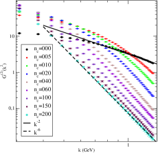
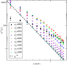
$\beta=5.8\ (24^{4})$
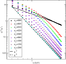
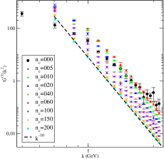
$\beta=6.0\ (32^{4})$

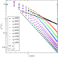
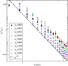
Figure 1: Evolution of $G^{(2)}(k^{2})$ (left) and $G^{(3)}(k^{2})$ (right) with cooling, a clear transition happens after a few cooling sweeps.

IV.1 Green functions

The first and more impressive hint we observe in the plots of fig. 1 is that both gluon propagator and vertex join the asymptotic classical behaviour predicted by Eq. (10) after a few cooling sweeps. In particular, for the gluon propagator (left plots), while in perturbation theory it decreases at high momentum, $k$, with $k^{-2}$ (except for the anomalous dimension logarithm), after killing quantum correlations we obtain a rather clean $k^{-6}$ behaviour. For the three-gluon vertex (right plots), correspondingly, we observe $k^{-10}$ instead of $k^{-6}$ after cooling. These observations allow to conclude that after cooling, correlations at high energies are dominated by instanton-like structures.

A second remarkable hint is how the asymptotic classical regime is reached: the higher is the number of cooling sweeps, the lower are the energies where both Green functions begin to behave as given by Eq. (10). As a matter of fact, the typical instanton size, $\rho$, grows with the cooling and the asymptotic formula Eq. (10) stands for $k\gg\rho^{-1}$. Furthermore, if we compare lattice data at different $\beta$ for the same number of cooling sweeps, we also qualitatively observe that the effect of cooling grows with the lattice spacing, $a(\beta)$, as expected after considering the cooling radius in Eq. (11) (the lower is $\beta$, the lower are the energies where the asymptotic behaviour is reached).

IV.2 Evolution with cooling

The effect of the cooling in terms of the cooling radius can be quantitatively analyzed because the instanton density can be extracted from a fit of the lattice data in the asymptotic regime to Eq. (4) for all the lattices and number of cooling sweeps. The asymptotic behaviour does not depend on the details of the instanton liquid, and is the same for any instanton profile or even for merons Lenz:2003jp . Thus, the fitted density should not be sensitive to the possible instanton deformations induced by the cooling.

In fig. 2, we present the evolution of the density with the number of cooling sweeps and with the cooling radius. The nice matching of the results for the three lattices proves that the estimated density through the fit to Eq. (10) indeed evolves with the correlation length introduced by the cooling. In other words, for the same cooling correlation length all our cooled lattice data match to each other and behave as classically predicted in Eq. (10).

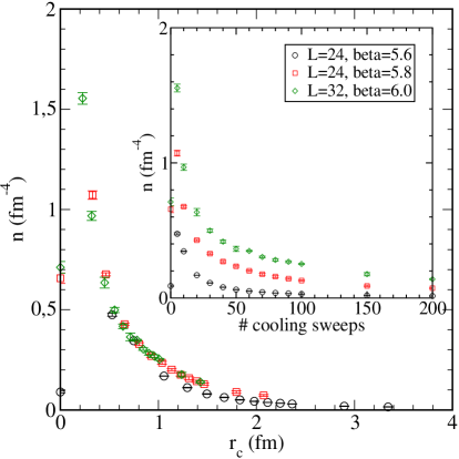
Figure 2: Density obtained from a fit of the lattice data for $G^{(3)}(k^{2})$ to the classical expresions (10). Different curves for different values of $\beta$ (detail) do coincide in terms of cooling radius.

IV.3 The running coupling

A final hint of plots in fig. 1 to be discussed is why the cooling procedure, supposed to destroy only short-distance correlations, immediately modify the low-momentum range of Green functions. This is because of the density damping induced by the cooling. The instanton profile depends of the instanton density Diakonov:1983hh ; Boucaud:2002fx and the low-momentum Green functions are affected by instanton profile effects Boucaud:2002fx , diverging as $k\to 0$ in the zero-density limit.

A simple manner of testing this explanation, with no detailed discussion about the instanton profile, is analyzing the QCD running coupling in Eq. (6). As we above discussed, if the radius-distribution width is small enough, the instanton-profile effects from two- and three-gluon Green function very approximatively cancel to each other in Eq. (6) and we recover a $k^{4}$-power law. We can write:

$$\alpha\left(k^{2}\right)\ =\ \frac{1}{18\pi n\overline{\rho}^{4}}\times\left\{\begin{array}[]{ll}c\left(k\overline{\rho}\right)^{4-\varepsilon}&k\overline{\rho}\ \raise 1.29167pt\hbox{$<$\kern-7.5pt\raise-4.73611pt\hbox{$\sim$}}\ 1\\ (k\overline{\rho})^{4}&k\overline{\rho}\gg 1\end{array}\right.\ .$$ (14)

The low-momentum limit is taken from Boucaud:2002fx , where $c\simeq 1.6$ and $\varepsilon\simeq 0.1-0.2$. Both were estimated for $0.4<k<0.9$ GeV with a instanton radius distribution taken from Diakonov:1983hh centered at $\overline{\rho}=1.5$ GeV and are rather independent of the choice for the particular profile function.

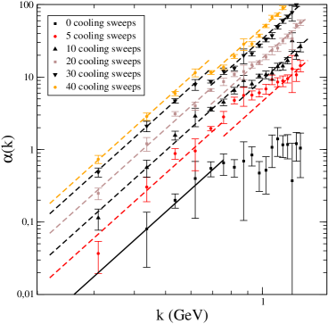
Figure 3: Log-log plot of the running coupling defined in Eq. (6) in terms of momenta. The two limits predicted by Eq. (14) are shown by straight and dashed lines respectively.

In fig. 3, the observance of the $k^{4}$-power law by the running coupling defined in Eq. (6) for both low and large-momentum range is manifest. We present, as an example, the results from the simulation at $\beta=5.6$ in a $24^{4}$ lattice, but the same is obtained from the other simulations. For the three lattices, the shifts of the straight line fitting the low-momentum data respect to the one fitting in large momenta correspond to $c\simeq 1.5-2.0$ defined in Eq. (14), in good agreement with results in Boucaud:2002fx . Consequently, densities plotted in fig. 2, obtained by fitting lattice data to the asymptotic formula Eq. (10) for large momenta, correspond in practice to the same fitted for low momenta in Boucaud:2002fx .

V Conclusions

In conclusion, after suppression of the short-distance correlations by cooling, the dominance of the semi-classical large-distance correlations leads to a nice description of the asymptotic behaviour of gluon Green functions within the instanton picture. In the low momentum range ($k\ \raise 1.29167pt\hbox{$<$\kern-7.5pt\raise-4.73611pt\hbox{$\sim$}}\ 1$ GeV), the cooling procedure only modifies details of the Instanton liquid like density or instanton profile. This can be seen by analyzing the QCD running coupling defined by Eq. (6) which shows the same classical pattern for both low and large momenta, as predicted by Eq. (14). Consequently, the low-momentum gluon Green functions from Montecarlo gauge configurations are determined by the classical correlations, although their description within the Instanton picture requires to know the details of the Instanton liquid.

We are especially indebted to O. Pène, J.P. Leroy and J. Micheli for comments and suggestions very valuable for the ellaboration of this letter. This work has been partially supported by a grant of the spanish Ministery of Education and Science.

References

- (1) T. Schafer and E. V. Shuryak, Rev. Mod. Phys. 70 (1998) 323
- (2) D. Diakonov and V. Y. Petrov, Nucl. Phys. B 245 (1984) 259.
- (3) J. J. Verbaarschot, Nucl. Phys. B 362 (1991) 33 [Erratum-ibid. B 386 (1991) 236].
- (4) M. Hutter, arXiv:hep-ph/0107098.
- (5) J. Glimm and A. Jaffe, Phys. Rev. Lett. 40 (1978) 277.
- (6) P. Boucaud, F. De Soto, A. Le Yaouanc, J. P. Leroy, J. Micheli, O. Pene and J. Rodriguez-Quintero, JHEP 0304, 005 (2003) and arXiv:hep-ph/0312332 (To be published)
- (7) F. Lenz, J. W. Negele and M. Thies, Phys. Rev. D 69 (2004) 074009; Contribution to Lattice04, arXiv:hep-th/0409083.
- (8) D. A. Smith and M. J. Teper [UKQCD collaboration], Phys. Rev. D 58 (1998) 014505
- (9) J. W. Negele, Nucl. Phys. Proc. Suppl. 73, 92 (1999)
- (10) I. Horvath et al., Phys. Rev. D 68 (2003) 114505
- (11) M. Teper. Phys. Lett., B162:357, 1985.
- (12) A. Ringwald and F. Schrempp, Phys. Lett. B 459 (1999) 249
- (13) D. Diakonov and V. Y. Petrov, Nucl. Phys. B 245, 259 (1984).
- (14)