LU TP 04-37

hep-ph/0410333

revised November 2004

Isospin Breaking in $K\to 3\pi$ Decays II:
Radiative Corrections

Johan Bijnens and Fredrik Borg
Department of Theoretical Physics, Lund University

Sölvegatan 14A, S 22362 Lund, Sweden

The five different CP conserving amplitudes for the decays $K\to 3\pi$ are calculated using Chiral Perturbation Theory. The calculation is made to next-to-leading order and includes full isospin breaking. The squared amplitudes are compared with the corresponding ones in the isospin limit to estimate the size of the isospin breaking effects. In this paper we add the radiative corrections to the earlier calculated $m_{u}-m_{d}$ and local electromagnetic effects. We find corrections of order 5-10 percent.

PACS numbers: 13.20.Eb; 12.39.Fe; 14.40.Aq; 11.30.Rd

1 Introduction

The non-perturbative nature of low-energy QCD calls for alternative methods of calculating processes including composite particles such as mesons and baryons. A method describing the interactions of the light pseudoscalar mesons ($K,\pi,\eta$) is Chiral Perturbation Theory (ChPT). It was introduced by Weinberg, Gasser and Leutwyler [1, 2, 3] and it has been very successful. Pedagogical introductions to ChPT can be found in [4]. The theory was later extended to also cover the weak interactions of the pseudoscalars [5], and the first calculation of a kaon decaying into pions ($K\to 2\pi,3\pi$) appeared shortly thereafter [6]. Reviews of other applications of ChPT to nonleptonic weak interactions can be found in [7].

A recalculation in the isospin limit of $K\to 2\pi$ to next-to-leading order was made in [8, 9] and of $K\to 3\pi$ in [9, 10]. In [9] also a full fit to all experimental data was made and it was found that the decay rates and linear slopes agreed well. However, a small discrepancy was found in the quadratic slopes and that is part of the motivation for this further investigation of the decay $K\to 3\pi$ in ChPT.

The discrepancies found can have several different origins. It could be an experimental problem or it could have a theoretical origin. In the latter case the corrections to the amplitude calculated in [9] are threefold: strong isospin breaking, electromagnetic (EM) isospin breaking or higher order corrections. These effects have been studied in many papers for the $K\to 2\pi$ decays, references can be traced back from [11]. For $K\to 3\pi$ less work has been done. In [12] the strong isospin and local electromagnetic corrections were investigated and it was found that the inclusion of those led to changes of a few percent in the amplitudes. The local electromagnetic part was also calculated in [10], in full agreement with our result after corrections of some misprints in [10].

In this paper we add also the radiative corrections, i.e. the nonlocal electromagnetic isospin breaking. The full (first order) isospin breaking amplitude to next-to-leading chiral order is thus calculated, and we will try to estimate the effect of this in the amplitudes. A new full fit, including also new experimental data [13, 14], has to be done to answer the question whether isospin breaking removes the problem of fitting the quadratic slopes. This, together with a study of models for the higher order coefficients, we plan to do in an upcoming paper.

Other recent results on $K\to 3\pi$ decays can be found in [15, 16]. In [15] Nicola Cabibbo discusses the possibility of determining the $a_{0}-a_{2}$ pion scattering length from the threshold effects of $K^{+}\to\pi^{0}\pi^{0}\pi^{+}$. He gives an approximate theoretical result with very few unknown parameters. We have a possibly better theoretical description of these effects but it includes more unknown parameters. In [16] an attempt was made to calculate the virtual photon corrections to the $K^{+}\to\pi^{0}\pi^{0}\pi^{+}$ decay. Our result disagrees with the result presented there.

The outline of this paper is as follows. The next section describes isospin breaking in more detail. In section 3 the basis of ChPT, the Chiral Lagrangians, are discussed. Section 4 specifies the decays and describes the relevant kinematics. The divergences appearing when including photons are discussed in section 5. In section 6 the analytical results are discussed, section 7 contains the numerical results and the last section contains the conclusions.

2 Isospin Breaking

Isospin symmetry is the symmetry under exchange of up- and down-quarks. Obviously this symmetry is only true in the approximation that $m_{u}=m_{d}$ and electromagnetism is neglected, i.e. in the isospin limit. Calculations are often performed in the isospin limit since this is simpler and gives a good first estimate of the result.

However, to get a precise result one has to include isospin breaking, i.e. the effects from $m_{u}\neq m_{d}$ and electromagnetism. Effects coming from $m_{u}\neq m_{d}$ we refer to as strong isospin breaking and include mixing between $\pi^{0}$ and $\eta$. This mixing leads to changes in the formulas for both the physical masses of $\pi^{0}$ and $\eta$ as well as the amplitude for any process involving either of the two. For a detailed discussion see [17].

The other source is electromagnetic isospin breaking, coming from the fact that the up- and the down-quarks are charged, which implies different interactions with photons. This part can be further divided in local electromagnetic isospin breaking and explicit photon contributions (radiative corrections). The former are described by adding new Lagrangians at each order and the latter by introducing new diagrams including photons.

Our first calculation of $K\to 3\pi$ [9] was done in the isospin limit. In the next paper, [12], we included strong and local isospin breaking (there collectively referred to as strong isospin breaking) and we now present the calculation including all isospin breaking effects.

3 The ChPT Lagrangians

The basis of our ChPT calculation is the various Chiral Lagrangians. They can be divided in different orders. The order parameters in the perturbation series are $p$ and $m$, the momenta and mass of the pseudoscalars. Including isospin breaking also $e$, the electron charge, and the mass difference, $m_{u}-m_{d}$, are used as order parameters. All of these are independent expansion parameters. We work to leading order in $m_{u}-m_{d}$ and $e^{2}$ but next-to-leading order in $p^{2}$ and $m^{2}$. For simplicity we call in the remainder terms of order $p^{2}$, $m^{2}$, $e^{2}$ and $m_{u}-m_{d}$ leading order, and terms of order $p^{4}$ ,$p^{2}\,m^{2}$, $m^{4}$, $p^{2}\,e^{2}$, $m^{2}\,e^{2}$, $p^{2}(m_{u}-m_{d})$ and $m^{2}(m_{u}-m_{d})$ next-to-leading order.

3.1 Leading Order

The leading order Chiral Lagrangian is usually divided in three parts

$${\cal L}_{2}={\cal L}_{S2}+{\cal L}_{W2}+{\cal L}_{E2},$$ (1)

where ${\cal L}_{S2}$ refers to the strong $\Delta S=0$ part, ${\cal L}_{W2}$ the weak $\Delta S=\pm 1$ part, and ${\cal L}_{E2}$ the strong-electromagnetic and weak-electromagnetic parts combined. For the strong part we have [2]

$${\cal L}_{S2}=\frac{F_{0}^{2}}{4}\;\langle u_{\mu}u^{\mu}+\chi_{+}\rangle$$ (2)

Here $\langle A\rangle$ stands for the flavour trace of the matrix $A$, and $F_{0}$ is the pion decay constant in the chiral limit. We define the matrices $u_{\mu}$, $u$ and $\chi_{\pm}$ as

$$u_{\mu}=iu^{\dagger}\,D_{\mu}U\,u^{\dagger}=u_{\mu}^{\dagger}\,,\quad u^{2}=U\,,\quad\chi_{\pm}=u^{\dagger}\chi u^{\dagger}\pm u\chi^{\dagger}u\,,$$ (3)

where the special unitary matrix $U$ contains the Goldstone boson fields

$$U=\exp\left(\frac{i\sqrt{2}}{F_{0}}M\right)\,,\quad M=\left(\begin{array}[]{ccc}\frac{1}{\sqrt{2}}\pi_{3}+\frac{1}{\sqrt{6}}\eta_{8}&\pi^{+}&K^{+}\\ \pi^{-}&\frac{-1}{\sqrt{2}}\pi_{3}+\frac{1}{\sqrt{6}}\eta_{8}&K^{0}\\ K^{-}&\overline{K^{0}}&\frac{-2}{\sqrt{6}}\eta_{8}\end{array}\right)\,.$$ (4)

The formalism we use is the external field method of [2], and to include photons we set

$$\chi=2B_{0}\left(\begin{array}[]{ccc}m_{u}&&\\ &m_{d}&\\ &&m_{s}\end{array}\right)\,\,\,\,\,\mathrm{and}\,\,\,\,D_{\mu}U=\partial_{\mu}U-ie\,QA_{\mu}U-ie\,UQA_{\mu},$$ (5)

where $A_{\mu}$ is the photon field and

$$Q=\left(\begin{array}[]{ccc}2/3&&\\ &-1/3&\\ &&-1/3\end{array}\right).$$ (6)

We diagonalize the quadratic terms in (2) by a rotation

$$\pi^{0} = \pi_{3}\cos\epsilon+\eta_{8}\sin\epsilon\,$$

$$\eta = -\pi_{3}\sin\epsilon+\eta_{8}\cos\epsilon\,,$$ (7)

where the lowest order mixing angle $\epsilon$ satisfies

$$\tan(2\epsilon)=\sqrt{3}\frac{m_{d}-m_{u}}{2\,m_{s}-m_{u}-m_{d}}\,.$$ (8)

The weak part of the Lagrangian has the form [18]

$${\cal L}_{W2}=C\,F_{0}^{4}\,\Bigg{[}G_{8}\langle\Delta_{32}u_{\mu}u^{\mu}\rangle+G_{8}^{\prime}\langle\Delta_{32}\chi_{+}\rangle+G_{27}t^{ij,kl}\,\langle\Delta_{ij}u_{\mu}\rangle\langle\Delta_{kl}u^{\mu}\rangle\Bigg{]}+\mbox{ h.c.}\,.$$

The tensor $t^{ij,kl}$ has as nonzero components

$$t^{21,13}=t^{13,21}=\frac{1}{3}\, \,t^{22,23}=t^{23,22}=-\frac{1}{6}\,;$$ ;

$$t^{23,33}=t^{33,23}=-\frac{1}{6}\, \,t^{23,11}=t^{11,23}=\frac{1}{3}\,,$$ ; (9)

and the matrix $\Delta_{ij}$ is defined as

$$\Delta_{ij}\equiv u\lambda_{ij}u^{\dagger}\,,\quad\left(\lambda_{ij}\right)_{ab}\equiv\delta_{ia}\,\delta_{jb}\,.$$ (10)

The coefficient $C$ is defined such that in the chiral and large $N_{c}$ limits $G_{8}=G_{27}=1$,

$$C=-\frac{3}{5}\,\frac{G_{F}}{\sqrt{2}}V_{ud}\,V_{us}^{*}=-1.06\cdot 10^{-6}\,\,\mathrm{GeV}^{-2}\,.$$ (11)

Finally, the remaining electromagnetic part, relevant for this calculation, looks like (see e.g. [19])

$${\cal L}_{E2}=e^{2}F_{0}^{4}Z\langle{\cal Q}_{L}{\cal Q}_{R}\rangle+e^{2}F_{0}^{4}\langle\Upsilon{\cal Q}_{R}\rangle$$ (12)

where the weak-electromagnetic term is characterized by a constant $G_{E}$ ($g_{\rm ewk}G_{8}$ in [19]),

$$\Upsilon=G_{E}\,F_{0}^{2}\Delta_{32}+{\rm h.c.}\,$$ (13)

and

$${\cal Q}_{L}=uQu^{\dagger}\,,\,\,\,{\cal Q}_{R}=u^{\dagger}Qu\,.$$ (14)

3.2 Next-to-leading Order

The fact that ChPT is a non-renormalizable theory means that new terms have to be added at each order to compensate for the loop-divergences. This means that the Lagrangians increase in size for every new order and the number of free parameters rises as well. At next-to-leading order the Lagrangian is split in four parts which, in obvious notation, are

$${\cal L}_{4}={\cal L}_{S4}+{\cal L}_{W4}+{\cal L}_{S2E2}+{\cal L}_{W2E2}(G_{8})\,.$$ (15)

Here the notation $(G_{8})$ indicates that here only the dominant $G_{8}$-part is included in the Lagrangian and therefore in the calculation.

These Lagrangians are quite large and we choose not to write them explicitly here since they can be found in many places [2, 20, 5, 21, 22, 19, 23]. For a list of all the pieces relevant for this specific calculation see [12]. Note however that four terms producing photon interactions should be added to ${\cal L}_{W4}$ in [12]. The two new terms in the octet part are

$$N_{14}\,i\,\langle\Delta_{32}\,\{f_{+}^{\mu\nu},u_{\mu}u_{\nu}\}\rangle\,+N_{15}\,i\,\langle\Delta_{32}\,u_{\mu}f_{+}^{\mu\nu}u_{\nu}\rangle$$ (16)

and in the 27 part

$$D_{13}\,i\,t^{ij,kl}\langle\Delta_{ij}\,u_{\mu}\rangle\langle\Delta_{kl}\,[u_{\nu},f_{+}^{\mu\nu}]\rangle\,+D_{15}\,i\,t^{ij,kl}\langle\Delta_{ij}\,u_{\mu}u_{\nu}\rangle\langle\Delta_{kl}\,f_{+}^{\mu\nu}\rangle,$$ (17)

where

$$f_{+}^{\mu\nu}=uF^{\mu\nu}u^{\dagger}+u^{\dagger}F^{\mu\nu}u,\,\,\,F^{\mu\nu}=e\,Q\,(\partial^{\mu}A^{\nu}-\partial^{\nu}A^{\mu}).$$ (18)

3.2.1 Ultraviolet Divergences

The process $K\to 3\pi$ receives higher-order contributions from diagrams that contain loops. The study of these diagrams is complicated by the fact that they need to be defined precisely. The loop-diagrams involve an integration over the undetermined loop-momentum $q$, and the integrals are divergent in the $q\rightarrow\infty$ ultraviolet region. These ultraviolet divergences are canceled by replacing the coefficients in the next-to-leading order Lagrangians by the renormalized coefficients and a subtraction part, see [9, 12] and references therein. The divergences can be used as a check on the calculation and all our infinities (except the ones left since the $G_{27}$-part in ${\cal L}_{W2E2}$ is not known) cancel as they should.

3.2.2 Loop Integrals

The prescription we use for the loop integrals can be found in many places, e.g. [24]. The only one needed in addition to the ones given there is the one-loop three point function

$$C(m_{1}^{2},m_{2}^{2},m_{3}^{3},p_{1}^{2},p_{2}^{2},p_{3}^{2})=\frac{1}{i}\int\frac{d^{d}p}{(2\pi)^{d}}\frac{1}{\left(p^{2}-m_{1}^{2}\right)\left((p-p_{1})^{2}-m_{2}^{2}\right)\left((p-p_{3})^{2}-m_{3}^{2}\right)}\,,$$ (19)

where $p_{3}=p_{1}+p_{2}$. For its numerical evaluation we use the program FF [25]. This program also deals with possible infrared divergences consistently.

4 Kinematics

There are five different CP-conserving decays of the type $K\to 3\pi$ ($K^{-}$ decays are not treated separately since they are counterparts to the $K^{+}$ decays):

$$K_{L}(k) \to \pi^{0}(p_{1})\,\pi^{0}(p_{2})\,\pi^{0}(p_{3})\,,\quad[A^{L}_{000}]\,,$$

$$K_{L}(k) \to \pi^{+}(p_{1})\,\pi^{-}(p_{2})\,\pi^{0}(p_{3})\,,\quad[A^{L}_{+-0}]\,,$$

$$K_{S}(k) \to \pi^{+}(p_{1})\,\pi^{-}(p_{2})\,\pi^{0}(p_{3})\,,\quad[A^{S}_{+-0}]\,,$$

$$K^{+}(k) \to \pi^{0}(p_{1})\,\pi^{0}(p_{2})\,\pi^{+}(p_{3})\,,\quad[A_{00+}]\,,$$

$$K^{+}(k) \to \pi^{+}(p_{1})\,\pi^{+}(p_{2})\,\pi^{-}(p_{3})\,,\quad[A_{++-}]\,,$$ (20)

where we have indicated the four-momentum defined for each particle and the symbol used for the amplitude.

The kinematics is treated using

$$s_{1}=\left(k-p_{1}\right)^{2}\,,\quad s_{2}=\left(k-p_{2}\right)^{2}\,,\quad s_{3}=\left(k-p_{3}\right)^{2}\,.$$ (21)

The amplitudes are expanded in terms of the Dalitz plot variables $x$ and $y$ defined as

$$y=\frac{s_{3}-s_{0}}{m_{\pi^{+}}^{2}}\,,\quad x=\frac{s_{2}-s_{1}}{m_{\pi^{+}}^{2}}\,,\quad s_{0}=\frac{1}{3}\left(s_{1}+s_{2}+s_{3}\right)\,.$$ (22)

The amplitude for $K_{L}\to\pi^{0}\pi^{0}\pi^{0}$ is symmetric under the interchange of all three final state particles and the one for $K_{S}\to\pi^{+}\pi^{-}\pi^{0}$ is antisymmetric under the interchange of $\pi^{+}$ and $\pi^{-}$ because of CP. The amplitudes for $K_{L}\to\pi^{+}\pi^{-}\pi^{0},K^{+}\to\pi^{+}\pi^{+}\pi^{-}$ and $K^{+}\to\pi^{0}\pi^{0}\pi^{+}$ are symmetric under the interchange of the first two pions because of CP or Bose-symmetry.

5 Infrared Divergences

In addition to the ultraviolet divergences which are removed by renormalization, diagrams including photons in the loops contain infrared (IR) divergences. These infinities come from the $q\rightarrow 0$ end of the loop-momentum integrals. They are canceled by including also the Bremsstrahlung diagram, where a real photon is radiated off one of the charged mesons, see Fig. 1. It is only the sum of the virtual loop corrections and the real Bremsstrahlung which is physically significant and thus needs to be well defined.

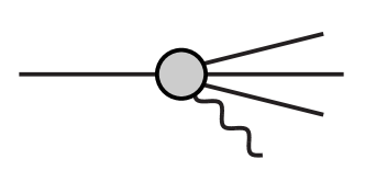
Figure 1: Bremsstrahlung, the emission of an extra final-state photon.

We regulate the IR divergence in both the virtual photon loops and the real emission with a photon mass $m_{\gamma}$ and keep only the singular terms plus those that do not vanish in the limit $m_{\gamma}\to 0$. We include the real Bremsstrahlung for photon energies up to a cut-off $\omega$ and treat it in the soft photon approximation.

The exact form of the amplitude squared for the bremsstrahlung diagram depends on which specific amplitude that is being calculated. For $K^{+}(k)\to\pi^{0}(p_{1})\pi^{0}(p_{2})\pi^{+}(p_{3})$ it can be written in the soft photon limit (see e.g. [26])

$$|A|^{2}_{BS}=|A|_{LO}^{2}\,e^{2}\,\int\frac{d^{3}q}{(2\pi)^{3}}\,\frac{1}{2q}\,\sum_{\lambda=0,1}\left[\frac{k\cdot\epsilon^{(\lambda)}}{q\cdot k}-\frac{p_{3}\cdot\epsilon^{(\lambda)}}{q\cdot p_{3}}\right]^{2},$$ (23)

where $|A|_{LO}$ is the lowest order isospin limit amplitude. The number of terms inside the parentheses is the number of charged particles in the process and the sign of those terms depends both on the charge of the radiating particle and on whether it is incoming or outgoing. Writing out the square and using $\sum_{\lambda=0,1}\epsilon^{(\lambda)}_{\mu}\epsilon^{(\lambda)}_{\nu}=-g_{\mu\nu}$, you get

$$|A|^{2}_{BS}=-|A|_{LO}^{2}\,e^{2}\,\int\frac{d^{3}q}{(2\pi)^{3}}\,\frac{1}{2q}\,\left[\frac{k^{2}}{(q\cdot k)^{2}}+\frac{p_{3}^{2}}{(q\cdot p_{3})^{2}}-\frac{2\,p_{3}\cdot k}{(q\cdot k)(q\cdot p_{3})}\right]$$ (24)

To solve the first integral term, place the vector $k$ along the z-axis, i.e.

$$k=(k^{0},0,0,k^{z})\,\,\,\mathrm{and}\,\,\,(k\cdot q)^{2}=(k^{0}q^{0}-k^{z}q^{z})^{2}.$$ (25)

Changing to polar coordinates that part of the integral now looks like

$$-|A|_{LO}^{2}\,e^{2}\,\frac{m_{K}^{2}}{8\pi^{2}}\int dq\,d(\cos\theta)\,\frac{q}{(k^{0}E_{\gamma}-k^{z}q\cos\theta)^{2}},$$ (26)

where $k^{2}=m_{K}^{2}$, $q_{0}=E_{\gamma}$ and $q_{z}=q\cos\theta$ have been used. Solving the $d(\cos\theta)$ part is now straightforward and leads to

$$-|A|_{LO}^{2}\,e^{2}\,\frac{m_{K}^{2}}{8\pi^{2}}\int dq\,\frac{1}{k^{z}}\left(\frac{1}{k^{0}E_{\gamma}-k^{z}q}-\frac{1}{k^{0}E_{\gamma}+k^{z}q}\right),$$ (27)

Putting the two terms on a common denominator and changing variable to $E_{\gamma}$ leads to

$$-|A|_{LO}^{2}\,e^{2}\,\frac{m_{K}^{2}}{4\pi^{2}}\int^{\omega}_{m_{\gamma}}dE_{\gamma}\frac{E_{\gamma}}{E_{\gamma}^{2}(k^{0})^{2}-(E_{\gamma}^{2}-m_{\gamma}^{2})(k^{z})^{2}}\,,$$ (28)

where $\omega$ is the photon energy above which the detector identifies it as a real external photon. We are only interested in the result in the limit $m_{\gamma}\to 0$, so it’s enough to consider

$$-|A|_{LO}^{2}\,e^{2}\,\frac{m_{K}^{2}}{4\pi^{2}}\int^{\omega}_{m_{\gamma}}dE_{\gamma}\frac{1}{m_{K}^{2}E_{\gamma}},$$ (29)

which gives the result

$$-|A|_{LO}^{2}\,\frac{e^{2}}{8\pi^{2}}\log\frac{\omega^{2}}{m_{\gamma}^{2}}\,.$$ (30)

In a similar way one gets the result for the mixed term

$$\int\frac{d^{3}q}{(2\pi)^{3}}\,\frac{1}{2q}\,\left[2\frac{p_{3}\cdot k}{(q\cdot k)(q\cdot p_{3})}\right]=-\frac{x_{s}}{4\pi^{2}}\frac{s_{3}-m_{K}^{2}-m_{\pi}^{2}}{m_{K}m_{\pi}(1-x_{s}^{2})}\log x_{s}\log\frac{\omega^{2}}{m_{\gamma}^{2}}\equiv I_{IR}(m_{K}^{2},m_{\pi}^{2},s_{3})\,,$$ (31)

where

$$x_{s}=\frac{\sqrt{1-4m_{K}m_{\pi}/(\bar{s}_{3}-(m_{K}-m_{\pi})^{2})}-1}{\sqrt{1-4m_{K}m_{\pi}/(\bar{s}_{3}-(m_{K}-m_{\pi})^{2})}+1}.$$ (32)

In order to obtain the correct imaginary part we use the $i\varepsilon$-prescription, which means $\bar{s}_{3}=s_{3}+i\varepsilon$.

For the other amplitudes the calculations are similar and the resulting bremsstrahlung amplitudes are

$$|A^{L}_{000}|^{2}_{BS}=0\,,$$ (33)

$$|A^{L}_{+-0}|^{2}_{BS}=-|A_{+-0}^{L}|^{2}_{LO}\,\frac{e^{2}}{4\pi^{2}}\,\left[\log\frac{\omega^{2}}{m_{\gamma}^{2}}-I_{IR}(m_{\pi}^{2},m_{\pi}^{2},s_{3})\right]\,,$$ (34)

$$|A^{S}_{+-0}|^{2}_{BS}=-|A^{S}_{+-0}|^{2}_{LO}\,\frac{e^{2}}{4\pi^{2}}\,\left[\log\frac{\omega^{2}}{m_{\gamma}^{2}}-I_{IR}(m_{\pi}^{2},m_{\pi}^{2},s_{3})\right]\,,$$ (35)

$$|A_{00+}|^{2}_{BS}=-|A_{00+}|^{2}_{LO}\,\frac{e^{2}}{4\pi^{2}}\,\left[\log\frac{\omega^{2}}{m_{\gamma}^{2}}-I_{IR}(m_{\pi}^{2},m_{K}^{2},s_{3})\right]\,,$$ (36)

$$|A_{++-}|^{2}_{BS} = -|A_{++-}|^{2}_{LO}\,\frac{e^{2}}{4\pi^{2}}\,\left[2\log\frac{\omega^{2}}{m_{\gamma}^{2}}-I_{IR}(m_{\pi}^{2},m_{K}^{2},s_{1})-I_{IR}(m_{\pi}^{2},m_{K}^{2},s_{2})\right.$$ (37)

$$+I_{IR}(m_{\pi}^{2},m_{K}^{2},s_{3})-I_{IR}(m_{\pi}^{2},m_{\pi}^{2},s_{1})-I_{IR}(m_{\pi}^{2},m_{\pi}^{2},s_{2})$$

$$\left.+I_{IR}(m_{\pi}^{2},m_{\pi}^{2},s_{3})\right]\,.$$

When using the above, the divergences from the explicit photon loops cancel exactly.

A similar problem shows up in the definition of the decay constants since we normalize the lowest order with $F_{\pi^{+}}$ and $F_{K^{+}}$. Our prescription for the decay constants is described in App. A.

6 Analytical Results

6.1 Lowest order

The four diagrams that could contribute to lowest order can be seen in Fig. 2.

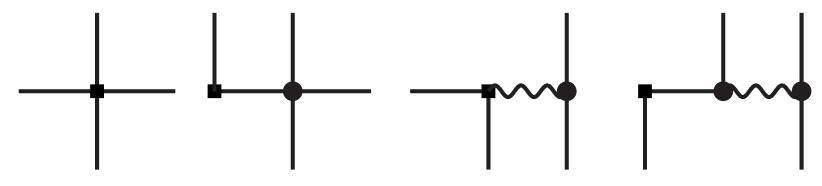
Figure 2: The tree level diagrams for $K\to 3\pi$. A filled square is a weak vertex, a filled circle a strong vertex, a straight line a pseudoscalar meson and a wiggly line a photon.

However, the two diagrams including photons turn out to give zero. This is obviously so for $K^{+}\to\pi^{+}\pi^{0}\pi^{0}$ and $K_{L}\to\pi^{0}\pi^{0}\pi^{0}$ since the $\gamma\pi^{0}\pi^{0}$ vertex vanishes as a consequence of charge conjugation.

The reason why it vanishes for the other decays is somewhat more subtle and is the same as why the lowest order result for $K\to\pi\ell^{+}\ell^{-}$ vanishes [27]. When doing a simultaneous diagonalization of the covariant kinetic and mass terms quadratic in the pseudoscalar fields, including those of the weak lagrangian ${\cal L}_{W2}$, $p^{2}$-terms of the form $\partial_{\mu}K\partial^{\mu}\pi$ are absent and all weak vertices involve at least three pseudoscalar fields. This result should not change as compared to our calculation where the weak Lagrangian was not included in the diagonalization. Thus in our case, the two diagrams on the right in Fig. 2 will together give zero contribution.

This means that the lowest order result in the full isospin case is the same as when just including strong and local EM isospin breaking. This result we published before, the full expressions can be found in [12].

6.2 Next-to-leading order

There are 51 additional diagrams contributing to next-to-leading order. They can be divided in three different classes and examples will be shown of each class. It should be noted that the argument in the previous subsection is not valid at this order. There now exist $K\pi\gamma$ vertices. The reason for this is that one can not diagonalize simultaneously all terms with two pseudoscalar fields when going to next-to-leading order.

The first class of diagrams are the 13 which do not include explicit photons. They are the ones used in our earlier papers [9, 12] and a complete list of them can be found there. Some examples are shown in Fig. 3.

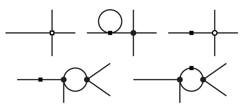
Figure 3: Examples of diagrams of next-to-leading order with no photons. An open square is a vertex from ${\cal L}_{W4}$ or ${\cal L}_{W2E2}$, an open circle a vertex from ${\cal L}_{S4}$ or ${\cal L}_{S2E2}$, a filled square a vertex from ${\cal L}_{W2}$ or ${\cal L}_{E2}\,(\Delta S=1)$ and a filled circle a vertex from ${\cal L}_{S2}$ or ${\cal L}_{E2}\,(\Delta S=0)$.

The second class of diagrams are the ones with a photon running in a loop. There are 18 of these and some examples can be found in Fig. 4. Their evaluation is the main new result of this paper. They are also responsible for the infrared divergences discussed in Sect. 5.

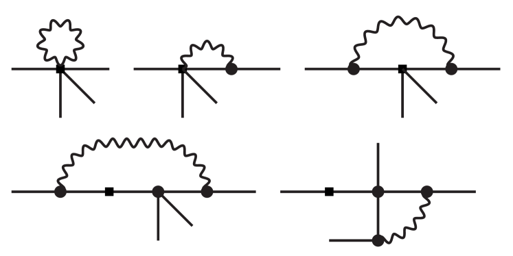
Figure 4: Examples of diagrams with photons in the loops. A filled square is a weak vertex, a filled circle a strong vertex, a straight line a pseudoscalar meson and a wiggly line a photon.

The first diagram is an example where the photon is the only particle in the loop, a photon tadpole diagram. These vanish in dimensional regularization when only singular and nonzero terms in the limit $m_{\gamma}\to 0$ are kept.

The last class of diagrams is the ones with tree level photon propagators, 20 in total. They are photon reducible, i.e. if we cut the photon line the diagram falls apart. They are infrared finite and some examples can be seen in Fig. 5. It turns out that for realistic values of the input parameters this class of diagrams give a negligible contribution to all $K\to 3\pi$ processes.

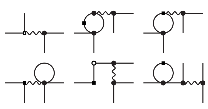
Figure 5: Examples of diagrams with photon propagators. An open square is a vertex from ${\cal L}_{W4}$ or ${\cal L}_{W2E2}$, an open circle a vertex from ${\cal L}_{S4}$ or ${\cal L}_{S2E2}$, a filled square a vertex from ${\cal L}_{W2}$ or ${\cal L}_{E2}\,(\Delta S=1)$ and a filled circle a vertex from ${\cal L}_{S2}$ or ${\cal L}_{E2}\,(\Delta S=0)$. A straight line is a pseudoscalar meson and a wiggly line a photon.

We work to first order in isospin breaking, i.e. as soon as $e^{2}$ is present we set $m_{u}=m_{d}$, $m_{\pi^{+}}=m_{\pi^{0}}=m_{\pi}$ and $m_{K^{+}}=m_{K^{0}}=m_{K}$. Even then, the resulting amplitudes at next-to-leading order are rather long, and it does not seem very useful to present them here explicitly. However, the full expressions for the amplitudes are available on request from the authors or can be downloaded [28]. It should be noted that the amplitude for $K_{L}\to\pi^{0}\pi^{0}\pi^{0}$ was given in [12]. It was stated that it was the full isospin breaking amplitude since no explicit photon diagrams can contribute to this process. This is not completely true, the amplitude will change indirectly through the definition of $F_{\pi^{+}}$ and $F_{K^{+}}$, see App. A.

The next-to-leading order amplitudes can in principle include all the low-energy coefficients (LECs) from ${\cal L}_{W4}$, ${\cal L}_{S4}$, ${\cal L}_{W2E2}$ and ${\cal L}_{S2E2}$. The coefficients from the strong and electromagnetic part of the Lagrangian are treated as input, which leaves $G_{8}$,$G_{27}$,$N^{r}_{1},\ldots,N^{r}_{13}$, $D^{r}_{1}$,$D^{r}_{2}$,$D^{r}_{4},\ldots,D^{r}_{7}$, $D^{r}_{26},\ldots,D^{r}_{31}$ and $Z^{r}_{1},\ldots,Z^{r}_{14}$ as undetermined. In total 41 unknown parameters. However, all of these do not appear independently, i.e. they multiply the same type of term, e.g. $m_{K}^{4}$ or $e^{2}m_{\pi}^{2}$. It turns out, as discussed in [12], that there are 30 independent combinations, denoted by $\tilde{K}_{1}\ldots\tilde{K}_{30}$. For the 11 combinations already appearing in the isospin limit see [9, 12] and the 19 additional ones for the isospin breaking case can be be found in [12]. In addition to the 30 combinations found in [12], four new coefficients show up when including photons: $N^{r}_{14}$, $N^{r}_{15}$, $D^{r}_{13}$ and $D^{r}_{15}$. These all come from the third class of diagrams where a tree level photon is present. The four coupling constants show up in precisely the same combinations in $K\to\pi\ell^{+}\ell^{-}$ and can thus be determined experimentally in other decays. We therefore treat them as input.

7 Numerical Results

7.1 Experimental data and fit

A full isospin limit fit was made in [9] taking into account all data published before May 2002. One of the motivations for this continued investigation of isospin breaking effects is to see whether isospin violation can solve the discrepancies in the quadratic slope parameters found there. A new full fit will be done in an upcoming paper. The data from ISTRA+ [13] and KLOE [14], which appeared after [9], will then also be taken into account. We do not present a new fit in this paper since estimates of the new combinations of constants should be done before attempting a full fit.

7.2 Inputs

$G_{8}$	$5.45$	$L_{1}^{r}$	$0.38\cdot 10^{-3}$	$\tilde{K}_{1}$	$0$
$G_{27}$	$0.392$	$L_{2}^{r}$	$1.59\cdot 10^{-3}$	$\tilde{K}_{2}/G_{8}$	$5.19\cdot 10^{-2}$
$G_{E}$	$-0.4$	$L_{3}^{r}$	$-2.91\cdot 10^{-3}$	$\tilde{K}_{3}/G_{8}$	$3.77\cdot 10^{-3}$
		$L_{4}^{r}$	$0$	$\tilde{K}_{4}$	0
$\sin\epsilon$	$1.19\cdot 10^{-2}$	$L_{5}^{r}$	$1.46\cdot 10^{-3}$	$\tilde{K}_{5}/G_{27}$	$-4.25\cdot 10^{-2}$
$Z$	$0.805$	$L_{6}^{r}$	$0$	$\tilde{K}_{6}/G_{27}$	$-1.66\cdot 10^{-1}$
$\mu$	0.77 GeV	$L_{7}^{r}$	$-0.49\cdot 10^{-3}$	$\tilde{K}_{7}/G_{27}$	$1.20\cdot 10^{-1}$
$F_{\pi}$	$0.0924$ GeV	$L_{8}^{r}$	$1.0\cdot 10^{-3}$	$\tilde{K}_{8}\ldots\tilde{K}_{11}$	0
$F_{K}$	$0.113$ GeV	$L_{9}^{r}$	$7.0\cdot 10^{-3}$	$\tilde{K}_{12}\ldots\tilde{K}_{30}$	$0$
$N_{14}$	$-10.4\cdot 10^{-3}$	$K_{1}\ldots K_{11}$	$0$	$D_{13}$	$0$
$N_{15}$	$5.95\cdot 10^{-3}$			$D_{15}$	$0$

Table 1: The various input values used.

The input values we use are presented in Table 1.

7.2.1 Strong and Electromagnetic Input

There are different ways to treat the masses, especially in the isospin limit case. In [9] the masses used in the phase space were obtained from the physical masses occuring in the decays. However in the amplitudes the physical mass of the kaon involved in the process was used and the pion mass was given by $m_{\pi}^{2}=\frac{1}{3}\sum_{i=1,3}m_{\pi^{i}}^{2}$ with $i=1,2,3$ being the three pions participating in the reaction. This allowed for the correct kinematical relation $s_{1}+s_{2}+s_{3}=m_{K}^{2}+3m_{\pi}^{2}$ to be satisfied while having the isospin limit in the amplitude but the physical masses in the phase space. The results in [9] were obtained with the physical mass for the eta. Results with the Gell-Mann-Okubo (GMO) relation for the eta mass in the loops gave small changes within the general errors given in [9].

In the decays here, we work to first order in isospin breaking. We have rewritten explicit factors of $m_{u}-m_{d}$ in terms of $\sin\epsilon$ according to

$$m_{u}-m_{d}=-\frac{2}{\sqrt{3}}\,\,(2\,m_{s}-m_{u}-m_{d})\,\sin\epsilon\,.$$ (38)

In general we use the physical masses of pions and kaons in the loops but as soon as a factor of $\sin\epsilon$ or $e^{2}$ is present we use a common kaon and a common pion mass. This simplifies the analytical formulas enormously. The kaon mass chosen is the mass from the kaon in the decay and the pion mass used is $3m_{\pi}^{2}=\sum_{i}m_{\pi^{i}}^{2}$ with $i=1,2,3$ the three pions in the final state, i.e. the mass we used in the isospin limit case. For the eta mass we use in general the GMO mass in the loops but with isospin violation included,

$$m_{\eta}^{2}=\frac{2}{3}\,(m_{K^{+}}^{2}+m_{K^{0}}^{2}-m_{\pi^{+}}^{2})+\frac{1}{3}\,m_{\pi^{0}}^{2}\,.$$ (39)

The possible lowest order contributions from the eta mass have been removed from the amplitudes using the corresponding next-to-leading order relation as described in [12].

The strong LECs $L_{1}^{r}$ to $L_{8}^{r}$ from ${\cal L}_{S4}$ as well as $\sin\epsilon$ come from the one-loop fit in [17].

The constant $Z$ from ${\cal L}_{E2}$ we estimate via

$$Z=\frac{1}{2\,F_{\pi}^{2}\,e^{2}}\,(m_{\pi^{+}}^{2}-m_{\pi^{0}}^{2}),$$ (40)

which corresponds to the value in Table 1. The higher order coefficients of ${\cal L}_{E4}$, $K_{1}\ldots K_{11}$, are rather unknown. Some rough estimates exist but we put them to zero here.

The IR divergences are cancelled by adding the soft-photon Bremsstrahlung. We have used a 10 MeV cut-off in energy for this and used the same cut-off in the definition of $F_{\pi^{+}}$ and $F_{K^{+}}$.

The subtraction scale $\mu$ is chosen to be $0.77$ GeV.

7.2.2 Weak Inputs

The coefficients contributing in the isospin limit from ${\cal L}_{W2}$ and ${\cal L}_{W4}$ are taken from the fit in [9]. The values of $G_{8}$, $G_{27}$ in Table 1 are taken from [9] as well. We use as a reasonable estimate for $G_{E}$ the value presented in [29].

No knowledge exists of the values of $\tilde{K}_{12}\ldots\tilde{K}_{30}$, so they are set equal to zero at $\mu=0.77$ GeV. Tests were also made assigning order of magnitude estimates to them. This imparted changes in the isospin breaking corrections similar in size to those of the loop contributions.

7.2.3 Input relevant for the Photon Reducible Diagrams

The two new constants $D_{13}$ and $D_{15}$ are set to zero since no knowledge exist of their values. Note that in order to contribute at all, they have to get values orders of magnitude larger than the expected size.

The two other new constants, $N_{14}$ and $N_{15}$, can be determined from $K\to\pi l^{+}l^{-}$ decays. For these decays, the branching ratios can be expressed as [27]

$$\mathrm{BR}(K^{+}\to\pi^{+}e^{+}e^{-}) = (3.15-21.1w_{+}+36.1w_{+}^{2})\cdot 10^{-8}\,|C\,G_{8}/(9\cdot 10^{-6}\cdot\mathrm{GeV}^{-2})|^{2}$$

$$\mathrm{BR}(K_{S}\to\pi^{0}e^{+}e^{-}) = (3.07-18.7w_{S}+28.4w_{S}^{2})\cdot 10^{-10}\,|C\,G_{8}/(9\cdot 10^{-6}\cdot\mathrm{GeV}^{-2})|^{2}$$

Using the measured central values [30]

$$\mathrm{BR}(K^{+}\to\pi^{+}e^{+}e^{-})=2.88\cdot 10^{-7},\,\,\,\mathrm{BR}(K_{S}\to\pi^{0}e^{+}e^{-})=3.0\cdot 10^{-9}$$ (42)

one gets the results

$$w_{+}^{(1)}=1.69,\,\,\,w_{+}^{(2)}=-1.10\,\,\,\,\,\mathrm{and}\,\,\,\,\,w_{S}^{(1)}=1.93,\,\,\,w_{S}^{(2)}=-1.28.$$ (43)

These constants, $w_{+}$ and $w_{S}$, can then be written in terms of both strong and weak low-energy constants [27],

$$w_{+} = \frac{4}{3}\,(4\pi)^{2}[N^{r}_{14}(\mu)-N^{r}_{15}(\mu)+3\,L^{r}_{9}(\mu)]-\frac{1}{3}\ln{\frac{m_{K}m_{\pi}}{\mu^{2}}}$$

$$w_{S} = \frac{2}{3}\,(4\pi)^{2}[2\,N^{r}_{14}(\mu)+N^{r}_{15}(\mu)]-\frac{1}{3}\ln{\frac{m_{K}^{2}}{\mu^{2}}},$$ (44)

and from the knowledge of $L^{r}_{9}(\mu)$ [31], one gets the values listed in Table 1 for one choice of signs in eq. (43).

Note that the influence of this class of diagrams is not visible in the figures nor in the results shown in the tables for any of the possible signs chosen in eq. (43). The magnitude of these constants needs to be increased significantly in order to have a visible impact on our numerical results.

7.3 Results with and without isospin breaking

The results we will present here is a comparison between the squared amplitudes and the decay rates in the isospin limit and including first order isospin breaking. The full squared amplitudes over the decay region is a 3-D plot with the two different cases plotted over phasespace. This is however very difficult to read, and instead we will present comparisons along three slices of these 3-D plots as explained below. We also present the corrections for the Dalitz plot parameters.

In Table 2 we present the values of the amplitudes squared in the center of the Dalitz plot, i.e. for $x=y=0$. We show the results in the isospin limit from [9], with the strong and local electromagnetic isospin breaking included [12] and with full isospin breaking included.

	Centralvalue
	Iso [9]	Strong [12]	Full
$K_{L}\to\pi^{0}\pi^{0}\pi^{0}$	$6.74\cdot 10^{-12}$	$6.97\cdot 10^{-12}$	$7.04\cdot 10^{-12}$
$K_{L}\to\pi^{+}\pi^{-}\pi^{0}$	$7.46\cdot 10^{-13}$	$7.66\cdot 10^{-13}$	$7.88\cdot 10^{-13}$
$K_{S}\to\pi^{+}\pi^{-}\pi^{0}$	$0$	$0$	$0$
$K^{+}\to\pi^{0}\pi^{0}\pi^{+}$	$0.93\cdot 10^{-13}$	$1.01\cdot 10^{-12}$	$1.03\cdot 10^{-12}$
$K^{+}\to\pi^{+}\pi^{+}\pi^{-}$	$3.72\cdot 10^{-12}$	$4.00\cdot 10^{-12}$	$4.14\cdot 10^{-12}$

Table 2: Comparison of the central values of the amplitudes squared in the isospin conserving case (Iso), including strong and local electromagnetic (Strong) and full (Full) isospin breaking.

Similarly, in Table 3 we present the integrated decay rates in the isospin conserving case [9], the one with strong and local electromagnetic isospin breaking included [12] and with all isospin breaking effects included. There are here in principle problems with an infinite correction when a charged two pion system is at rest. The effects of the electromagnetic interaction can then become very large from terms containing logarithms of the pion velocity. This is where the Coulomb interaction dominates and it should then really be resummed to all orders. In order to avoid this problem we have introduced the cut-off $E_{C}$. It means that we only integrate the phase space over the part where

$$\sqrt{s_{i}}\geq 2m_{\pi}+E_{C}\,.$$ (45)

Due to the way we have chosen the pion mass, the Coulomb problem only shows up for the decay $K^{+}\to\pi^{+}\pi^{+}\pi^{-}$ where the systems of two charged pions can be at rest or at very low relative velocity at the edges of phase space. The places where this happens are indicated by the large dots in Fig. 6. The choice of the pion masses in $K_{L,S}\to\pi^{+}\pi^{-}\pi^{0}$ is such that the Coulomb threshold is slightly outside the physical phasespace. It turns out that in this case the part of the correction that includes the Coulomb singularity is rather small. We have therefore not included any corrections for it in the results presented.

	Decay Rate
	Iso [9]	Strong	Full	$E_{C}$ [MeV]
$K_{L}\to\pi^{0}\pi^{0}\pi^{0}$	$2.65\cdot 10^{-18}$	$2.74\cdot 10^{-18}$	$2.77\cdot 10^{-18}$
$K_{L}\to\pi^{+}\pi^{-}\pi^{0}$	$1.63\cdot 10^{-18}$	$1.67\cdot 10^{-18}$	$1.72\cdot 10^{-18}$
$K_{S}\to\pi^{+}\pi^{-}\pi^{0}$	$3.1\cdot 10^{-21}$	$3.2\cdot 10^{-21}$	$3.3\cdot 10^{-21}$
$K^{+}\to\pi^{0}\pi^{0}\pi^{+}$	$9.11\cdot 10^{-19}$	$9.84\cdot 10^{-19}$	$1.00\cdot 10^{-18}$
$K^{+}\to\pi^{+}\pi^{+}\pi^{-}$	$2.97\cdot 10^{-18}$	$3.19\cdot 10^{-18}$	—	0
	$2.95\cdot 10^{-18}$	$3.17\cdot 10^{-18}$	$3.28\cdot 10^{-18}$	1
	$2.91\cdot 10^{-18}$	$3.13\cdot 10^{-18}$	$3.24\cdot 10^{-18}$	2
	$2.72\cdot 10^{-18}$	$2.93\cdot 10^{-18}$	$3.03\cdot 10^{-18}$	5

Table 3: Comparison of the decay rates in the isospin conserving case (Iso), including strong and local electromagnetic (Strong) and full (Full) isospin breaking. The Coulomb cut-off used, $E_{C}$, is explained in the text.

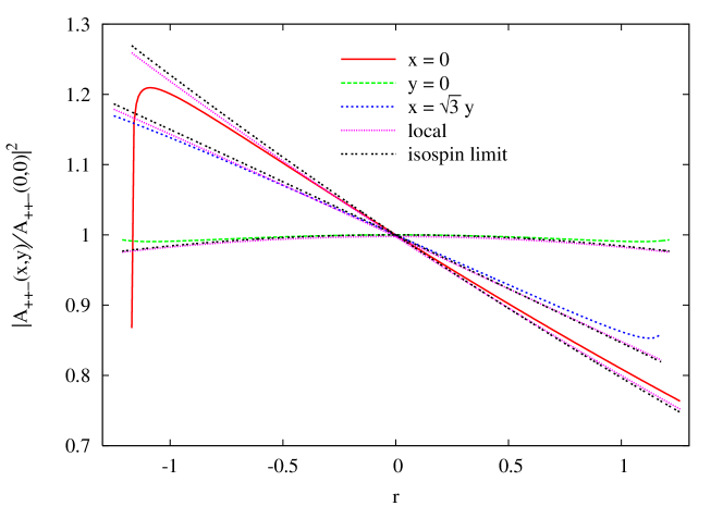
Figure 11: Comparison of $K^{+}\to\pi^{+}\pi^{+}\pi^{-}$ with and without isospin breaking.

In Fig. 6 we also show the phase space boundaries for the five different decays and the three curves along which we will show results for the squared amplitudes with and without isospin breaking. The three curves are $x=0$, $y=0$ and $x=\sqrt{3}\,y$. In Fig. 7 to Fig. 11 we then plot the five different squared amplitudes along these curves as a function of $r$, where $r=\pm\sqrt{y^{2}+\frac{x^{2}}{3}}$ and the sign is chosen according to

$$r=\left\{\begin{array}[]{ll}y,&x=0\\ x/\sqrt{3},&y=0\\ y\,\sqrt{2},&x=y\,\sqrt{3}\,.\end{array}\right.$$ (46)

Note that for all but $A^{S}_{+-0}$ the squared amplitudes are normalized to their value at the center of the Dalitz plot. A comparison of the central values themselves is shown in Table 2.

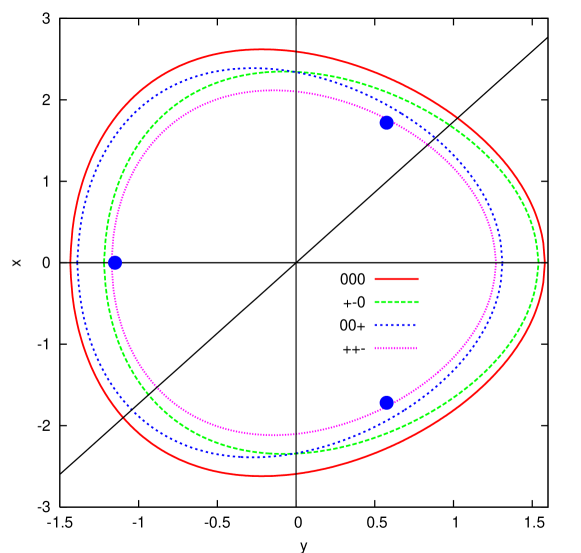
Figure 6: The phase space boundaries for the five different decays and the three curves along which we will compare the squared amplitudes. The points where two charged pions have low relative velocity for $K^{+}\to\pi^{+}\pi^{+}\pi^{-}$ are indicated by the large dots.

We also calculate the changes in the Dalitz plot distribution parameters. These are defined by

$$\left|\frac{A(s_{1},s_{2},s_{3})}{A(s_{0},s_{0},s_{0})}\right|^{2}=1+gy+hy^{2}+kx^{2}\,.$$ (47)

The isospin breaking corrections to these parameters are given in Table 4. The amplitude for $K_{S}\to\pi^{+}\pi^{-}\pi^{0}$ is parametrized via

$$A^{S}_{+-0}=\gamma_{S}x-\xi_{S}xy\,.$$ (48)

Decay	Quantity	Iso [9]	Strong	Full
$K_{L}\to\pi^{0}\pi^{0}\pi^{0}$	$h$	$-0.0072$	$-0.0068$	$-0.0068$
$K_{L}\to\pi^{+}\pi^{-}\pi^{0}$	$g$	0.673	0.683	0.677
	$h$	0.085	0.089	0.088
	$k$	0.0055	0.0057	0.0057
$K_{S}\to\pi^{+}\pi^{-}\pi^{0}$	$\gamma_{S}$	$3.4\cdot 10^{-8}$	$3.4\cdot 10^{-8}$	$3.5\cdot 10^{-8}$
	$\xi_{S}$	$-0.2\cdot 10^{-8}$	$-0.2\cdot 10^{-8}$	$-0.2\cdot 10^{-8}$
$K^{+}\to\pi^{0}\pi^{0}\pi^{+}$	$g$	0.635	0.619	0.619
	$h$	0.074	0.071	0.071
$K^{+}\to\pi^{+}\pi^{+}\pi^{-}$	$g$	$-0.215$	$-0.211$	$-0.201$
	$h$	0.012	0.012	0.008
	$k$	$-0.0052$	$-0.0050$	$-0.0037$

Table 4: Comparison of the Dalitz plot distribution parameters in the isospin conserving case (Iso), including strong and local electromagnetic (Strong) and full (Full) isospin breaking.

We now discuss the results in somewhat more detail. In general the results are of a size as can be expected from this type of isospin breaking. They are of order a few, up to 11% in the amplitudes squared outside the Coulomb region. The isospin breaking corrections tend to increase all decay rates somewhat and this will in a fit be compensated by small changes in the values of the $\tilde{K}_{i}$ compared to the results of [9]. The number of significant digits quoted in Table 2 is higher than the expected precision of our results, but the trend and the general size of the change compared to the isospin conserving results are stable with respect to variations in dealing with the eta mass (physical or GMO).

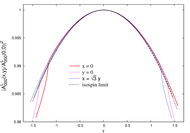
Figure 7: Comparison of $K_{L}\to\pi^{0}\pi^{0}\pi^{0}$ with and without isospin breaking.

For $K_{L}\to\pi^{0}\pi^{0}\pi^{0}$ the central value of the amplitude squared increases by about 4.5%. In this case we have because of the symmetry of the final state that $g=0$ and $k=h/3$. The quadratic slope decreases by about 5% but the total variation over the Dalitz plot is small so the total decay rate increases by about 4.5% as well. This decay is the one which has most variation in the amplitude when changing how one deals with the eta mass. The extreme case we have found was that this effect completely cancelled the change from isospin violation, but the relative change due to isospin breaking remained similar. Note the scale in Fig. 7 when viewing the result. The changes compared to [12] are entirely due to the photon loop corrections to $F_{\pi^{+}}$ and $F_{K^{+}}$.

In Fig. 7 one can also clearly see the thresholds induced by the difference between $m^{2}_{\pi^{+}}$ and $m^{2}_{\pi^{0}}$ introduced when isospin invariance is broken. These thresholds correspond to a new process being allowed where two of the neutral pions are produced through an intermediate on shell state with one positive and one negative pion.

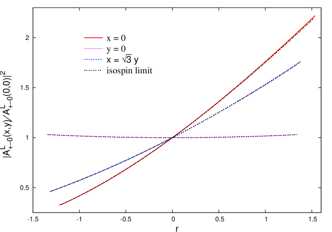
Figure 8: Comparison of $K_{L}\to\pi^{+}\pi^{-}\pi^{0}$ with and without isospin breaking.

The squared amplitude $K_{L}\to\pi^{+}\pi^{-}\pi^{0}$ increases by about 5.5% with very little variation with the eta mass treatment. The decay rate increases by the same amount. The changes in the Dalitz plot slopes are rather small as can be judged from Fig. 8. The marginal differences compared to $g$ quoted in [9] are due to a slightly different fitting procedure to the amplitudes squared.

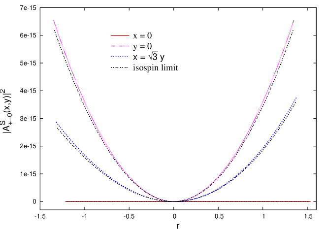
Figure 9: Comparison of $K_{S}\to\pi^{+}\pi^{-}\pi^{0}$ with and without isospin breaking.

For the decay $K_{S}\to\pi^{+}\pi^{-}\pi^{0}$ the amplitude in the center of the Dalitz plot vanishes because of the symmetries. The amplitude and the slopes increase by about 3% as can be seen in Fig. 9 and the tables.

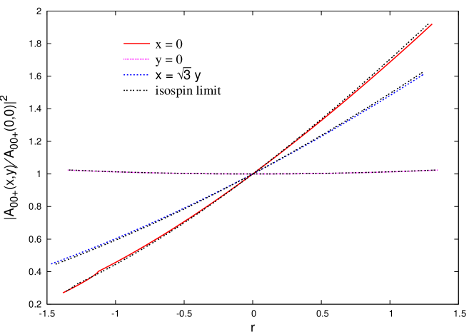
Figure 10: Comparison of $K^{+}\to\pi^{0}\pi^{0}\pi^{+}$ with and without isospin breaking.

The decay $K^{+}\to\pi^{0}\pi^{0}\pi^{+}$ has a large increase. The squared amplitude in the center changes by about 11%. The linear slopes decrease somewhat leading to an increase of about 10% to the total decay rate when compared with the isospin conserved case. This is shown in Fig. 10.

The amplitude for $K^{+}\to\pi^{0}\pi^{0}\pi^{+}$ is also calculated in [16]. Our results don’t agree with the numerics presented there. We find an increase in the amplitude while there a decrease is found. In [16] a different choice of lowest order was made than here and in [9, 12]. After taking that difference into account, we still disagree significantly with the numerical results of [16].

The decay $K^{+}\to\pi^{+}\pi^{+}\pi^{-}$ has a change of about 11% upwards in the center of the Dalitz plot. The slopes decrease somewhat. The decay rate can only be compared when the Coulomb region is excluded from the comparison but the total change is also about 11%.

The conclusions above do not change qualitatively when we give the $K_{i}^{r}$ a value of about $0.001$ and the new isospin breaking $\tilde{K}_{i}$ a value relative to $G_{8}$ and $G_{27}$ of $0.01$. However the changes induced by these values are numerically significant. They can be of the order of 10%, largest for $K_{L}\to\pi^{0}\pi^{0}\pi^{0}$.

It should be noted that the mentioned changes are with the values of $\tilde{K}_{i}$ determined from the isospin conserving fit in [9]. A new determination including isospin breaking effects is planned in an upcoming paper.

8 Conclusions

We have calculated the $K\to 3\pi$ amplitudes to next-to-leading order ($p^{4},p^{2}\,m^{2},m^{4},p^{2}\,e^{2}$) in Chiral Perturbation Theory. A similar calculation was done in [9] in the isospin limit, and in [12] including strong isospin breaking, but we have now included full isospin breaking. The motivations for this are both because it is interesting in general to see the importance of isospin breaking in this process, but also to investigate whether isospin violation will improve the fit to experimental data. Discrepancies between data and the quadratic slopes from ChPT were found in [9], and isospin breaking may be the cause of this.

We have estimated the effects of the isospin breaking by comparing the squared amplitudes with and without isospin violation. The effect seems to be at 5-10% percent level in the amplitudes squared. To investigate if this removes the discrepancies found in [9] a new full fit has to be done, also including the new data [13, 14] published after [9]. This is work in progress and will be presented in the future paper Isospin Breaking in $K\to 3\pi$ Decays III.

Appendix A The Decay constants $F_{\pi^{+}}$ and $F_{K^{+}}$.

We have chosen to normalize our lowest order contribution with $F_{0}^{4}/(F_{\pi^{+}}^{3}F_{K^{+}})$. $F_{\pi^{+}}$ and $F_{K^{+}}$ are the pion and kaon decay constants respectively. Including isospin breaking they are determined from the diagrams in Fig. 12 and the resulting expressions are

Figure 12: Diagrams for the decay constants. An open square is a vertex from ${\cal L}_{W4}$ or ${\cal L}_{W2E2}$, a filled square a vertex from ${\cal L}_{W2}$ or ${\cal L}_{E2}\,(\Delta S=1)$ and a filled circle a vertex from ${\cal L}_{S2}$ or ${\cal L}_{E2}\,(\Delta S=0)$. A straight line is a pseudoscalar meson and a wiggly line a photon.

$$F_{\pi^{+}}=F_{0}\Bigg{\{}1+\frac{1}{F_{0}^{2}}\Bigg{[}$$ (A.1)

$$F_{0}^{2}e^{2}\,\Big{(}4/3\,K^{r}_{1}+4/3\,K^{r}_{2}+10/9\,K^{r}_{5}+10/9\,K^{r}_{6}+2\,K^{r}_{12}$$

$$+2\,\frac{\partial}{\partial q^{2}}\overline{B}(m_{\gamma}^{2},m_{\pi}^{2},m_{\pi}^{2})\,m_{\pi}^{2}-\overline{B}_{1}(m_{\gamma}^{2},m_{\pi}^{2},m_{\pi}^{2})-2\,\frac{\partial}{\partial q^{2}}\overline{B}_{1}(m_{\gamma}^{2},m_{\pi}^{2},m_{\pi}^{2})\,m_{\pi}^{2}\Big{)}$$

$$+L^{r}_{4}\,\Big{(}16\,m_{\pi}^{2}\,\frac{\sin\epsilon}{\sqrt{3}}-16\,m_{K}^{2}\,\frac{\sin\epsilon}{\sqrt{3}}+4\,m_{\pi^{0}}^{2}+8\,m_{K^{0}}^{2}\Big{)}$$

$$+L^{r}_{5}\,\Big{(}4\,m_{\pi^{0}}^{2}\Big{)}+1/2\,\overline{A}(m_{\pi^{+}}^{2})+1/2\,\overline{A}(m_{\pi^{0}}^{2})+1/4\,\overline{A}(m_{K^{+}}^{2})+1/4\,\overline{A}(m_{K^{0}}^{2})\Bigg{]}\Bigg{\}}$$

and

$$F_{K^{+}}=F_{0}\Bigg{\{}1+\frac{1}{F_{0}^{2}}\Bigg{[}$$ (A.2)

$$F_{0}^{2}\,e^{2}\,\Big{(}4/3\,K^{r}_{1}+4/3\,K^{r}_{2}+10/9\,K^{r}_{5}+10/9\,K^{r}_{6}+2\,K^{r}_{12}$$

$$+2\,\frac{\partial}{\partial q^{2}}\overline{B}(m_{\gamma}^{2},m_{K}^{2},m_{K}^{2})\,m_{K}^{2}-\overline{B}_{1}(m_{\gamma}^{2},m_{K}^{2},m_{K}^{2})-2\,\frac{\partial}{\partial q^{2}}\overline{B}_{1}(m_{\gamma}^{2},m_{K}^{2},m_{K}^{2})\,m_{K}^{2}\Big{)}$$

$$+L^{r}_{4}\,\Big{(}16\,m_{\pi}^{2}\,\frac{\sin\epsilon}{\sqrt{3}}-16\,m_{K}^{2}\,\frac{\sin\epsilon}{\sqrt{3}}+4\,m_{\pi^{0}}^{2}+8\,m_{K^{0}}^{2}\Big{)}$$

$$+L^{r}_{5}\,\Big{(}16\,m_{\pi}^{2}\,\frac{\sin\epsilon}{\sqrt{3}}-16\,m_{K}^{2}\,\frac{\sin\epsilon}{\sqrt{3}}+4\,m_{K^{0}}^{2}\Big{)}$$

$$+3/4\,\frac{\sin\epsilon}{\sqrt{3}}\,\overline{A}(m_{\pi}^{2})+1/4\,\overline{A}(m_{\pi^{+}}^{2})+1/8\,\overline{A}(m_{\pi^{0}}^{2})$$

$$+1/2\,\overline{A}(m_{K^{+}}^{2})+1/4\,\overline{A}(m_{K^{0}}^{2})+\overline{A}(m_{\eta}^{2})\,\Big{(}3/8-3/4\,\frac{\sin\epsilon}{\sqrt{3}}\Big{)}\Bigg{]}\Bigg{\}}\,.$$

These formulas agree with known results [3, 33].

The above formulas are infrared divergent when $m_{\gamma}\to 0$, and the standard way to deal with this is the same as in the amplitudes, i.e. adding a bremsstrahlung diagram. We have chosen to just add a term including a cut-off scale for the bremsstrahlung photon,

$$-|A|_{LO}\,\frac{e^{2}}{4\pi^{2}}\,\log\frac{\omega^{2}_{F}}{m_{\gamma}^{2}}\,,$$ (A.3)

which cancels the dependence on the photon mass and therefore removes the divergence. The scale $\omega_{F}$ is set to $10\,\mathrm{MeV}$.

References

- [1] S. Weinberg, Physica A 96 (1979) 327.
- [2] J. Gasser and H. Leutwyler, Annals Phys. 158 (1984) 142.
- [3] J. Gasser and H. Leutwyler, Nucl. Phys. B 250 (1985) 465.
-
[4]
A. Pich, Lectures at Les Houches Summer School in
Theoretical Physics, Session 68: Probing the Standard Model of Particle
Interactions, Les Houches, France, 28 Jul - 5 Sep 1997,
[hep-ph/9806303];
G. Ecker, Lectures given at Advanced School on Quantum Chromodynamics (QCD 2000), Benasque, Huesca, Spain, 3-6 Jul 2000, [hep-ph/0011026]. - [5] J. Kambor, J. Missimer and D. Wyler, Nucl. Phys. B 346 (1990) 17.
- [6] J. Kambor, J. Missimer and D. Wyler, Phys. Lett. B 261 (1991) 496.
-
[7]
G. Ecker,
Prog. Part. Nucl. Phys. 35 (1995) 1,
[hep-ph/9501357];
A. Pich, Rept. Prog. Phys. 58 (1995) 563, [hep-ph/9502366];
E. de Rafael, Lectures given at Theoretical Advanced Study Institute in Elementary Particle Physics (TASI 94): CP Violation and the limits of the Standard Model, Boulder, CO, 29 May - 24 Jun 1994, [hep-ph/9502254]. - [8] J. Bijnens, E. Pallante and J. Prades, Nucl. Phys. B 521 (1998) 305, [hep-ph/9801326].
- [9] J. Bijnens, P. Dhonte and F. Persson, Nucl. Phys. B 648 (2003) 317, [hep-ph/0205341].
- [10] E. Gamiz, J. Prades and I. Scimemi, JHEP 0310 (2003) 042 [hep-ph/0309172].
-
[11]
J. Bijnens and M. B. Wise,
Phys. Lett. B 137 (1984) 245;
B. R. Holstein, Phys. Rev. D 20 (1979) 1187;
S. Gardner and G. Valencia, Phys. Rev. D 62 (2000) 094024, [hep-ph/0006240],
C. E. Wolfe and K. Maltman, Phys. Lett. B 482 (2000) 77 [hep-ph/9912254];
V. Cirigliano, J. F. Donoghue and E. Golowich, Phys. Lett. B 450 (1999) 24;
V. Cirigliano, G. Ecker, H. Neufeld and A. Pich, Eur. Phys. J. C 33 (2004) 369 [hep-ph/0310351]. - [12] J. Bijnens and F. Borg, Nucl. Phys. B 697 (2004) 319 [hep-ph/0405025].
- [13] I. V. Ajinenko et al., Phys. Lett. B 567, 159 (2003) [hep-ex/0205027].
- [14] A. Aloisio et al. [KLOE Collaboration], hep-ex/0307054.
- [15] N. Cabibbo, [hep-ph/0405001].
- [16] A. Nehme, [hep-ph/0406209].
- [17] G. Amorós, J. Bijnens, P. Talavera Nucl. Phys. B 602 (2001) 87,[hep-ph/0101127].
- [18] J. A. Cronin, Phys. Rev. 161 (1967) 1483.
- [19] G. Ecker, G. Isidori, G. Muller, H. Neufeld and A. Pich, Nucl. Phys. B 591 (2000) 419, [hep-ph/0006172].
- [20] V. Cirigliano, M. Knecht, H. Neufeld, H. Rupertsberger and P. Talavera, Eur. Phys. J. C 23, 121 (2002) [hep-ph/0110153].
- [21] G. Esposito-Farese, Z. Phys. C 50 (1991) 255.
- [22] G. Ecker, J. Kambor and D. Wyler, Nucl. Phys. B 394 (1993) 101, [hep-ph/0006172].
- [23] R. Urech, Nucl. Phys. B 433, 234 (1995) [hep-ph/9405341].
- [24] G. Amorós, J. Bijnens and P. Talavera, Nucl. Phys. B 568 (2000) 319, [hep-ph/9907264].
- [25] G. J. van Oldenborgh, Comput. Phys. Commun. 66 (1991) 1; G. J. van Oldenborgh and J. A. M. Vermaseren, Z. Phys. C 46 (1990) 425.
- [26] M. Peskin and D. Schroeder, “An Introduction to quantum field theory,” Perseus Books, Reading MA, USA (1995).
- [27] G. Ecker, A. Pich and E. de Rafael, Nucl. Phys. B 291 (1987) 692.
-
[28]
These can be downloaded
from
http://www.thep.lu.se/~bijnens/chpt.html. - [29] J. Bijnens and J. Prades, JHEP 0006 (2000) 035 [hep-ph/0005189].
- [30] S. Eidelman et al. [Particle Data Group Collaboration], Phys. Lett. B 592, 1 (2004).
- [31] J. Bijnens and P. Talavera, JHEP 0203 (2002) 046 [hep-ph/0203049].
- [32] J. A. Vermaseren, math-ph/0010025.
- [33] H. Neufeld and H. Rupertsberger, Z. Phys. C 71 (1996) 131 [hep-ph/9506448].