New Higgs Effects in B–Physics in Supersymmetry
with General Flavour Mixing

John Foster^a, Ken-ichi Okumura^b and Leszek Roszkowski<sup>a

a</sup> Department of Physics and Astronomy, University of Sheffield, Sheffield, UK

^b Department of Physics, KAIST, Daejeon, 305-701,Korea

1 Introduction

Flavour changing neutral current (FCNC) processes provide a promising place to look for possible signals of physics beyond the Standard Model (SM). This is because the GIM mechanism ensures that the SM contributions and additional effects due to “new physics” both enter at the one–loop level. As such the increasingly accurate experimental data obtained from dedicated $B$–factories as well as collider experiments can be used to place constraints on masses and other parameters of a given new physics model.

The process that provides some of the strictest constraints on physics beyond the SM is $\bar{B}\to X_{s}\gamma$. The current world average for the branching ratio is given by [1]

$${\rm BR}(\bar{B}\to X_{s}\gamma)_{\rm exp} =(3.52\pm 0.30)\times 10^{-4} E_{\gamma}>\frac{1}{20}m_{b}.$$

The SM prediction for the branching ratio for the decay is based on a next–to–leading order (NLO) calculation that was completed in Refs. [2, 3]

$${\rm BR}(\bar{B}\to X_{s}\gamma)_{\rm SM} =(3.70\pm 0.30)\times 10^{-4} E_{\gamma}>\frac{1}{20}m_{b}.$$

Using the recent results for the decay $\bar{B}\to X_{s}l^{+}l^{-}$, the sign of the $\bar{B}\to X_{s}\gamma$ amplitude can also be determined [5] to be that of the SM contribution. These results allow further constraints to be placed on any new physics beyond the SM that feature large contributions from additional sources of flavour violation.

Studies of physics beyond the SM such as supersymmetry (SUSY) have, until recently, typically focused on the inclusion of leading order (LO) effects (for example, see Ref. [6]). However, due to the increasing accuracy of experimental data and its relatively good agreement with the SM prediction it is becoming necessary to include at least the dominant effects that occur beyond the LO.

Such effects have been studied, for example, in the two Higgs doublet model (2HDM) and the Minimal Supersymmetric Standard Model (MSSM). The 2HDM calculation was completed in Refs. [7, 8]. Studies of the MSSM contributions have tended to focus on various approximations and specific schemes. For instance, the results presented in Ref. [9] assume minimal flavour violation (MFV) and a particle spectrum in which the charginos and one of the top squarks are lighter than the rest of the superpartners. In Refs. [10, 11] the effect of large $\tan\beta$–enhanced beyond leading order (BLO) corrections to the $b$–quark mass and charged Higgs coupling on the process $\bar{B}\to X_{s}\gamma$ was explored and shown to be sizable, and a resummation of terms proportional to $\alpha_{s}\tan\beta$ was performed to keep perturbation expansion under control. These methods were extended to include neutral Higgs contributions and $\tan\beta$–enhanced corrections to the tree–level CKM matrix in Ref. [12], general electroweak contributions and ${\rm SU}(2)_{L}\times{\rm U}(1)_{Y}$ breaking effects in Ref. [13] and the effects of general flavour mixing (GFM) in the soft sector in Ref. [14].

The calculation presented in Ref. [14] was based on constructing an effective field theory where the supersymmetric particles are integrated out at a scale $\mu_{SUSY}$ (in a similar manner to Ref. [10]). The down quark tree–level (or, in the language of Ref. [14], “bare”) mass matrix and the effective couplings were then calculated in the context of GFM. It was found that taking into account these effects can significantly reduce the bounds on the flavour violating parameters compared to purely LO calculations as a result of a “focusing effect” [14].

In this Letter we extend and generalise the methods presented in [14] to $\bar{B}_{s}-B_{s}$ mixing and the decay $\bar{B}_{s}\to\mu^{+}\mu^{-}$. Whilst the mass difference $\Delta M_{B_{s}}$ and the branching ratio BR($\bar{B}_{s}\to\mu^{+}\mu^{-}$) have so far remained undetermined, both processes provide possible places to look for signals of physics beyond the SM. In particular, large regions of the MSSM in the regime of large $\tan\beta$ can be explored. Since $B$–factories do not run at the energy required to produce large quantities of the $B_{s}$ mesons, the best experimental constraints on both processes are provided by collider experiments. The current experimental bound for the process $\bar{B}_{s}\to\mu^{+}\mu^{-}$ is provided by the DØ group at the Tevatron [15]

$${\rm BR}(\bar{B}_{s}\to\mu^{+}\mu^{-})_{\rm exp} <5.0\times 10^{-7} 95\%{\rm~{}C.L},$$

whilst the experimental bound on $\Delta M_{B_{s}}$ is [1]

$$\Delta M_{B_{s}}^{\rm exp} >14.5{\rm ps}^{-1} 95\%{\rm~{}C.L}.$$

The SM contributions to these processes are known to NLO [17, 18]. However, the largest source of error for both quantities is due to the hadronic matrix element $f_{B_{s}}$ which has to be determined using either lattice calculations or QCD sum rules. The values given in the literature for the branching ratio for the process $\bar{B}_{s}\to\mu^{+}\mu^{-}$ therefore tend to vary but are typically of the order [19]

$${\rm BR}(\bar{B}_{s}\to\mu^{+}\mu^{-})_{\rm SM}=(3.2\pm 1.5)\times 10^{-9}.$$ (1)

The SM prediction for $\Delta M_{B_{s}}$ is [20]

$$\Delta M_{B_{s}}^{\rm SM}=18.0\pm 3.7{\rm ps}^{-1},$$ (2)

where the large hadronic uncertainty has been avoided by using the experimentally measured value of $\Delta M_{d}^{\rm SM}$. It has also been pointed out that in models with minimal flavour violation the large uncertainty associated with the branching ratio for the decays $\bar{B}_{q}\to\mu^{+}\mu^{-}$ can also be avoided by relating it to the experimentally measured values of $\Delta M_{B_{q}}$ [21].

The contributions due to effects beyond the SM on the decay $\bar{B}_{s}\to\mu^{+}\mu^{-}$ arise due to contributions to $Z$ and Higgs penguins as well as box diagrams mediated by charginos and (in the GFM framework) neutralinos. The contributions due to neutral Higgs penguins in particular have been the subject of intense theoretical investigation [22, 23, 24, 25, 27, 28, 12, 13] recently due to the $\tan^{6}\beta$ dependence of ${\rm BR}(\bar{B}_{s}\to\mu^{+}\mu^{-})$. At large $\tan\beta$ it is therefore quite possible for ${\rm BR}(\bar{B}_{s}\to\mu^{+}\mu^{-})$ to be enhanced by a few orders of magnitude compared to the SM value, whilst still satisfying current experimental bounds and the restrictions imposed by $\bar{B}\to X_{s}\gamma$. Similar contributions arise in the $\bar{B}_{s}-B_{s}$ system, where the double Higgs penguin diagram, although strictly an NLO effect, can become comparable to the LO contributions in the large $\tan\beta$ limit [30, 27, 13].

In this Letter, in addition to the effects discussed in [14], we include the contributions of charginos and neutralinos when calculating corrections to the bare quark mass matrix and corrected vertices. We also include the effects of the modified neutral Higgs vertex when evaluating the contributions to $\bar{B}\to X_{s}\gamma$. For all three processes: $\bar{B}_{s}-B_{s}$ mixing and the decays $\bar{B}\to X_{s}\gamma$ and $\bar{B}_{s}\to\mu^{+}\mu^{-}$, we take into account all $\tan\beta$–enhanced corrections, the additional electroweak and ${\rm SU}(2)_{L}\times{\rm U}(1)_{Y}$ breaking effects discussed in [13] and the effects of GFM mixing parameters on the bare mass matrix [14].

2 GFM and $\tan\beta$–Enhanced Corrections

The effects of $\tan\beta$–enhanced SUSY corrections to the down quark Yukawa coupling [32] and the charged Higgs coupling [10, 11] have been found to be large and their inclusion can produce sizable deviations from purely LO calculations. As has been pointed out in Refs. [22, 24, 12, 13], these corrections can also affect the structure of the CKM matrix, K, due to the additional unitary transformations required to transform the quark fields into a super–CKM basis.

To illustrate this consider the effect of integrating out the SUSY particles on the down quark mass matrix. The physical down quark masses (denoted $m_{d}$) are given in terms of the uncorrected quark masses (denoted $m_{d}^{(0)}$) by the relation

$$m_{d}=m_{d}^{(0)}+\delta m_{d}.$$ (3)

Note that, relative to Ref. [14], we have dropped the factor $\alpha_{s}/4\pi$ in front of $\delta m_{d}$ because here we will also include chargino and neutralino corrections, in addition to the (dominant) SUSY QCD ones considered in Ref. [14].

In the physical super–CKM basis the mass matrix $m_{d}$ is (by definition) diagonal, but in general $m_{d}^{(0)}$ (and $\delta m_{d}$) is not and provides a source of flavour violation. Alternatively [22, 24, 12, 13], one can start with the “bare” super–CKM basis where $m_{d}^{(0)}$ is diagonal and, after computing the corrections, diagonalise the corrected mass matrix, which amounts to rotating to the physical super–CKM basis. In this approach flavour violation is introduced via unitary rotation matrices as they affect the CKM matrix, as well as the various other vertices present in the resulting effective theory.

In the limit of MFV both approaches can be shown to be equivalent. For example, the $1+\epsilon_{s}\tan\beta$ dependence (where $\epsilon_{s}$ will be defined shortly) that arises when the CKM matrix is modified in the approach described in Refs. [22, 24, 12, 13] is reproduced once the gluino contributions to a given process are taken into account. When performing MFV calculations the method presented in Ref. [13] is more convenient since the gluino corrections to a given vertex are solely to the flavour diagonal terms. However, in GFM scenarios the flavour violating gluino (and neutralino) contributions are evaluated anyway. Additionally the iterative procedure described in Ref. [14] is more suited to calculations where the squark mass matrix is diagonalised numerically.

Here we follow the procedure described in Ref. [14]. The bare mass matrix $m_{d}^{(0)}$ and the corrections to the electroweak vertices are calculated in the physical super–CKM basis using an iterative procedure. The supersymmetric contributions to the process in question are then evaluated, taking into account the effects of the modified bare mass matrix, and evolved from $\mu_{SUSY}$ to the electroweak scale $\mu_{W}$ using the relevant six flavour anomalous dimension matrix. The electroweak contributions are then evaluated, using the uncorrected vertices when evaluating the NLO corrections and the corrected vertices when evaluating the LO contributions. Finally the combined supersymmetric and electroweak Wilson coefficients are evolved from $\mu_{W}$ to $\mu_{b}$ using the five flavour anomalous dimension matrix and used to calculate the relevant observable for the process in question.

Before presenting our numerical results it will be useful to consider the effects of including GFM contributions when calculating $m_{d}^{(0)}$ and the resulting effects on the Wilson coefficients relevant to $\bar{B}\to X_{s}\gamma$, $\bar{B}_{s}\to\mu^{+}\mu^{-}$ or $\bar{B}_{s}-B_{s}$ mixing. To this end we work in the mass insertion approximation (MIA) where the off–diagonal entries of the $6\times 6$ squark mass matrix are treated as perturbations and flavour violation is communicated through mixed propagators proportional to the appropriate off–diagonal element. In our numerical analysis MIA is not assumed and all the squark mass matrices are diagonalised numerically.

Departures from MFV can be measured in terms of the parameters $\delta_{LL}$, $\delta_{LR}$, $\delta_{RL}$ and $\delta_{LR}$ definitions of which can be found in Ref. [14]. If one delta is varied at a time the diagonal terms of the bare mass matrix are given by the well known result [32]

$$\left(m_{d}^{(0)}\right)_{ii}=\frac{\left(m_{d}\right)_{ii}}{1+\left(\epsilon_{s}+\delta_{i3}\epsilon_{Y}Y_{t}^{2}\right)\tan\beta},$$ (4)

where $i=1,2,3$ (or $d$, $s$, $b$), $Y_{t}$ is the Yukawa coupling of the top quark and the presence of the Kronecker $\delta$–function $\delta_{i3}$ reflects the fact that the chargino contribution proportional to the top quark Yukawa coupling only effects the bottom quark mass. (Corrections to the strange and down quark masses are suppressed by $K_{ts}K_{ts}^{\ast}$ and $K_{td}K_{td}^{\ast}$, respectively, and are set equal to zero.) Finally,

$$\epsilon_{s} =-\frac{\alpha_{s}}{2\pi}C_{2}(3)\frac{\mu}{m_{\tilde{g}}}H_{2}(x_{\tilde{d}_{R}},x_{\tilde{d}_{L}}), \epsilon_{Y} =-\frac{A_{t}}{16\pi^{2}\mu}H_{2}(y_{\tilde{u}_{R}},y_{\tilde{u}_{L}}),$$ (5)

where $\alpha_{s}$ is the strong coupling constant, $C_{2}(3)=4/3$ is the quadratic Casimir operator for $SU(3)$, $\mu$ is the Higgs/higgsino mass parameter, $m_{\tilde{g}}$ is the gluino mass and $A_{t}$ is the $3,3$ element of the trilinear up–type soft term. The loop function $H_{2}$ can be found in the Appendix. Its arguments and some other quantities to appear below are defined as

$$x_{\tilde{d}_{L,R}} =\frac{\widetilde{m}_{d,LL,RR}^{2}}{m_{\tilde{g}}^{2}}, x_{\tilde{d}_{RL}} =\frac{\sqrt{\widetilde{m}_{d,LL}^{2}}\sqrt{\widetilde{m}_{d,RR}^{2}}}{m_{\tilde{g}}^{2}}, y_{\tilde{u}_{L,R}} =\frac{\widetilde{m}_{u,LL,RR}^{2}}{\mu^{2}},$$ (6)

where $\widetilde{m}^{2}_{d,LL}$, $\widetilde{m}^{2}_{d,RR}$ denote common values of the diagonal entries of $3\times 3$ squark soft SUSY breaking terms for which we follow the conventions given in Ref. [14]. Whilst the diagonal elements of the soft terms have been assumed to be universal, it is relatively easy to include the effects of flavour dependence at the cost of clarity in the final expressions.

It has been pointed out in Ref. [29] that if $\delta_{LL}$ and $\delta_{RR}$ are both non–zero large corrections to the bare strange and down quark masses can occur at third order in the MIA. In our numerical analysis we diagonalise the squark mass matrix numerically and therefore these corrections are automatically included.

Taking into account flavour violating effects in the LR sector and ignoring the effects induced by other sources of flavour violation (including the CKM matrix) the off–diagonal elements of $m_{d}^{(0)}$ are given by (a more complete formula will be given in Ref. [33])

$$\left(m_{d}^{(0)}\right)_{ij}=\frac{\epsilon_{RL}}{1+\left(\epsilon_{s}+\epsilon_{Y}Y_{t}^{2}\delta_{j3}\right)\tan\beta}\;x_{\tilde{d}_{RL}}m_{\tilde{g}}\left(\delta_{RL}\right)_{ij}+\mathcal{O}(\delta^{3})$$ (7)

where $i,j=1,2,3$ and

$$\epsilon_{RL}=-\frac{\alpha_{s}}{2\pi}C_{2}(3)H_{2}(x_{\tilde{d}_{R}},x_{\tilde{d}_{L}}).$$ (8)

The effect of including GFM corrections to $m_{d}^{(0)}$ and the electroweak vertices can be rather large. For example, in the case of $\bar{B}\to X_{s}\gamma$ the presence of non–zero $\left(m_{d}^{(0)}\right)_{32}$ can lead to large corrections to $\delta^{\chi^{-}}C_{7,8}$ that are otherwise suppressed by a factor of $K_{cb}m_{b}$ [14]. Similarly $\left(m_{d}^{(0)}\right)_{23}$ induces analogous corrections to the chargino contributions in the primed sector that are usually suppressed by $m_{s}K_{ts}^{\ast}$.

In the case of $\bar{B}_{s}\to\mu^{+}\mu^{-}$, the gluino contributions to the Wilson coefficients of the scalar and pseudoscalar operators become (in the large $\tan\beta$ limit)

$$\delta^{\tilde{g}}C_{S,P}=\pm\frac{4\alpha_{s}}{3\alpha}\frac{\mu m_{\mu}}{m_{A}^{2}{m}_{b}m_{\tilde{g}}}\frac{\tan^{3}\beta}{K_{tb}K_{ts}^{\ast}}\bigg{[} \left(m_{d}^{(0)}\right)_{32}^{\ast}H_{2}(x_{\tilde{d}_{R}},x_{\tilde{d}_{L}})$$

$$+ \left(m_{d}^{(0)}\right)_{33}^{\ast}\left(\delta_{LL}\right)_{23}x_{\tilde{d}_{L}}H_{3}(x_{\tilde{d}_{R}},x_{\tilde{d}_{L}},x_{\tilde{d}_{L}})\bigg{]},$$ (9)

where $m_{\mu}$ denotes the mass of the $\mu$–lepton, whilst the primed coefficients are given by

$$\delta^{\tilde{g}}C_{S,P}^{\prime}=\frac{4\alpha_{s}}{3\alpha}\frac{\mu m_{\mu}}{m_{A}^{2}{m}_{s}m_{\tilde{g}}}\frac{\tan^{3}\beta}{K_{tb}K_{ts}^{\ast}}\bigg{[} \left(m_{d}^{(0)}\right)_{23}H_{2}(x_{\tilde{d}_{L}},x_{\tilde{d}_{R}})$$

$$+ \left(m_{d}^{(0)}\right)_{33}\left(\delta_{RR}\right)_{23}x_{\tilde{d}_{R}}H_{3}(x_{\tilde{d}_{L}},x_{\tilde{d}_{R}},x_{\tilde{d}_{R}})\bigg{]},$$ (10)

(for details of the operator basis we use see Ref. [26]). Substituting Eq. (4) and Eq. (7) into the above expressions yields the Wilson coefficients:

$$\delta^{\tilde{g}}C_{S,P}= \pm\frac{4\alpha_{s}}{3\alpha}\frac{\mu m_{\mu}}{m_{A}^{2}}\frac{\tan^{3}\beta}{K_{tb}K_{ts}^{\ast}}\Bigg{\{}\frac{\epsilon_{RL}}{[1+\epsilon_{s}\tan\beta]}\frac{x_{\tilde{d}_{RL}}}{m_{b}}\left(\delta_{LR}\right)_{23}H_{2}(x_{\tilde{d}_{R}},x_{\tilde{d}_{L}})$$

$$+ \frac{1}{[1+\epsilon_{s}\tan\beta][1+\left(\epsilon_{s}+\epsilon_{Y}Y_{t}^{2}\right)\tan\beta]}\frac{x_{\tilde{d}_{L}}}{m_{\tilde{g}}}\left(\delta_{LL}\right)_{23}H_{3}(x_{\tilde{d}_{R}},x_{\tilde{d}_{L}},x_{\tilde{d}_{L}})\Bigg{\}},$$ (11)

$$\delta^{\tilde{g}}C_{S,P}^{\prime}= \frac{4\alpha_{s}}{3\alpha}\frac{\mu m_{\mu}}{m_{A}^{2}}\frac{\tan^{3}\beta}{K_{tb}K_{ts}^{\ast}}\Bigg{\{}\frac{[\epsilon_{RL}+\frac{m_{\tilde{g}}}{\mu}\epsilon_{Y}Y_{t}^{2}]}{[1+\left(\epsilon_{s}+\epsilon_{Y}Y_{t}^{2}\right)\tan\beta]}\frac{x_{\tilde{d}_{RL}}}{m_{s}}\left(\delta_{RL}\right)_{23}H_{2}(x_{\tilde{d}_{L}},x_{\tilde{d}_{R}})$$

$$+\frac{1}{[1+\left(\epsilon_{s}+\epsilon_{Y}Y_{t}^{2}\right)\tan\beta]^{2}}\frac{x_{\tilde{d}_{R}}}{m_{\tilde{g}}}\frac{m_{b}}{m_{s}}\left(\delta_{RR}\right)_{23}H_{3}(x_{\tilde{d}_{L}},x_{\tilde{d}_{R}},x_{\tilde{d}_{R}})\Bigg{\}},$$ (12)

where $m_{A}$ denotes the mass of the pseudoscalar Higgs boson and $\alpha$ denotes the electromagnetic coupling constant.

Comparing the above expressions with the analysis of Ref. [27], the term in Eq. (4.15) proportional to the insertion $\delta_{LL}$ needs to be corrected by a factor

$$\frac{1+\left(\epsilon_{s}+\epsilon_{Y}Y_{t}^{2}\right)\tan\beta}{1+\epsilon_{s}\tan\beta}$$ (13)

which reflects the additional contribution (which was omitted in Ref. [27]) obtained when including the effects of the insertion on the bare CKM matrix.

Values of up to $\mathcal{O}(1)$ for both $\delta_{LL}$ and $\delta_{RR}$ are viable in some regions of parameter space [34] and can lead to large contributions to $C_{S}^{(\prime)}$ and $C_{P}^{(\prime)}$. Large values of $\delta_{RR}$, in particular, are motivated by $SO(10)$ or $SU(5)$ based solutions [35, 36] to the neutrino mass problem. As well as these corrections, the insertions $\delta_{LR}$ and $\delta_{RL}$ reappear once BLO effects are taken into account. At LO the insertions vanish due to an accidental cancellation between the self energy and vertex corrections to the effective Higgs vertex. Including BLO effects however, allows the insertions to appear through their effects on the bare mass matrix Eq. (7). This effect is independent of the LO cancellation and originates from the additional unitary transformations that are required to transform between the bare super–CKM basis and the physical super–CKM basis. Additionally, since the corrections proportional to $\delta_{LR}$ and $\delta_{RL}$ depend on $m_{\tilde{g}}$, rather than the strange or bottom quark mass, the enhancement by $m_{\tilde{g}}/m_{b}$ can compensate for the $\alpha_{s}^{2}$–dependence of the Wilson coefficient.

As discussed in Ref. [13] the corrected neutral Higgs vertex can effect $\bar{B}_{s}-B_{s}$ mixing via double Higgs penguin diagrams that contribute to the Wilson coefficients of the operators

$$\mathcal{O}^{LR}_{2}= (b^{\alpha}P_{L}s^{\alpha})(b^{\beta}P_{R}s^{\beta}), \mathcal{O}^{SLL}_{1}= (b^{\alpha}P_{L}s^{\alpha})(b^{\beta}P_{L}s^{\beta}), \mathcal{O}^{SRR}_{1}= (b^{\alpha}P_{R}s^{\alpha})(b^{\beta}P_{R}s^{\beta}).$$ (14)

(for details of the operator basis we use see Ref. [31]). In the large $\tan\beta$ regime the dominant contribution arises from the Wilson coefficient $C^{LR}_{2}$, as the pseudoscalar and scalar contributions approximately cancel for both $C^{SLL}_{1}$ and $C^{SRR}_{1}$. For non–zero $\delta_{LL}$ and $\delta_{LR}$ the contributions to $C^{LR}_{2}$ are typically suppressed by a factor of the strange quark mass. For the insertions $\delta_{RR}$ and $\delta_{RL}$, however, it is possible to avoid this suppression factor via the diagram where one Higgs penguin is mediated by chargino exchange and the other by gluino exchange. In the case of non–zero $\delta_{RR}$, for example, $C^{LR}_{2}$ is given by

$$C^{LR}_{2}=-\frac{8\alpha_{s}}{3\pi^{2}\alpha\sin^{2}\theta_{W}}\frac{A_{t}Y_{t}^{2}m_{b}^{2}}{m_{\tilde{g}}m_{A}^{2}}\frac{\tan^{4}\beta}{K_{tb}^{\ast}K_{ts}}\;\kappa\,\left(\delta_{RR}\right)_{23}\,x_{\tilde{d}_{R}}H_{2}(y_{\tilde{u}_{R}},y_{\tilde{u}_{L}})H_{3}(x_{\tilde{d}_{L}},x_{\tilde{d}_{R}},x_{\tilde{d}_{R}}),$$ (15)

where $\kappa$ contains the effects of resuming $\tan\beta$ enhanced contributions

$$\kappa=\frac{1}{(1+\epsilon_{s}\tan\beta)\times[1+(\epsilon_{s}+\epsilon_{Y}Y_{t}^{2})\tan\beta]^{3}}.$$ (16)

Figure 1: BR($\bar{B}_{s}\to\mu^{+}\mu^{-}$) vs. $\delta_{RR}$ (on the left) and vs. $\delta_{RL}$ (on the right).The soft sector is parameterised in terms of a common mass for the squark soft terms $m_{\tilde{q}}$, $m_{\tilde{g}}=\sqrt{2}m_{\widetilde{q}}=1\,\mbox{TeV}$, $A_{t}=-1\,\mbox{TeV}$, $m_{H^{+}}=\mu=500\,\mbox{GeV}$ and the gaugino soft terms $M_{1}=M_{2}=0.5m_{\tilde{g}}$, for $\tan\beta=50$.

3 Numerical Results

When performing our numerical calculations we diagonalise all the various mixing matrices numerically, whilst we use FeynHiggs 2.0.2 [37] to compute the parameters associated with the Higgs sector. Fig. 1 shows the effects of including beyond leading order GFM contributions on the decay $\bar{B}_{s}\to\mu^{+}\mu^{-}$ and its dependence on the flavour violating parameters $\delta_{RR}$ and $\delta_{RL}$. For $\delta_{RR}$ the effect of using the bare bottom quark mass, as well as the additional effects induced by the off–diagonal elements of $m_{d}^{(0)}$ present in Eq. (10), reduce the contribution to the decay by about a factor of two. A similar reduction between the LO and BLO results occurs for the insertion $\delta_{LL}$. This reduction of LO effects by the inclusion of BLO supersymmetric corrections can be viewed as an extension of the focusing effect found in Ref. [14] to the neutral Higgs vertex. For $\delta_{RL}$ (and similarly $\delta_{LR}$) the effects are more dramatic. As stated above, at leading order the contribution due to $\delta_{RL}$ cancels and the remaining contributions stem from Z penguin diagrams that are not enhanced at large $\tan\beta$. However, once BLO corrections are taken into account the effects can differ quite significantly from the LO scenario where the dominant contributions at large $\tan\beta$ arise from the chargino contributions to the neutral Higgs vertex.

Figure 2: $\Delta M_{B_{s}}$ vs. $\delta_{RR}$ (on the left) and vs. $\delta_{RL}$ (on the right) for the same parameters as in Fig. 1.

Fig. 2 shows a similar plot for the $\bar{B}_{s}-B_{s}$ system. The strong linear dependence on both $\delta_{RL}$ and $\delta_{RR}$ confirms the approximate formula presented in the previous section. The effect of including BLO contributions once again has a large effect. Both graphs are somewhat similar to their $\bar{B}_{s}\to\mu^{+}\mu^{-}$ analogs underlining the dependence on the corrected Higgs vertex and the large effects it can display in the large $\tan\beta$ region. For $\delta_{RR}$ the effect of including BLO contributions can once again lessen the dependence on $\delta_{RR}$ with respect to a purely LO analysis and lead to values of $\Delta M_{B_{s}}$ closer to the SM prediction. In the case of the insertion $\delta_{RL}$, the effect of including BLO contributions is once again rather large and can lead to large deviations from a purely LO calculation.

From Figs. 1–2 it is evident that the inclusion of BLO effects can significantly reduce both BR($\bar{B}_{s}\to\mu^{+}\mu^{-}$) and $\Delta M_{B_{s}}$ relative to LO predictions in the case of the insertion $\delta_{RR}$. This focusing effect can be viewed as an extension of the results presented in Ref. [14] to the neutral Higgs vertex. Fig. 3 illustrates the strong correlation between $\Delta M_{B_{s}}$ and BR($\bar{B}_{s}\to\mu^{+}\mu^{-}$) at large $\tan\beta$ reflecting the fact that both processes are highly dependent on the neutral Higgs coupling in this regime.

Figure 3: A scatter plot of BR($\bar{B}_{s}\to\mu^{+}\mu^{-}$) vs. $\Delta M_{B_{s}}$ for $0.2<|\delta_{RR}|<0.5$ and $\tan\beta=40$.

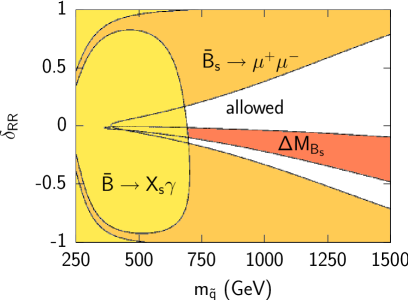
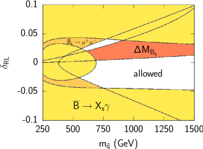
Figure 4: In the above plots the region excluded by $\bar{B}\to X_{s}\gamma$ is shaded in yellow (light grey). The additional regions excluded by $\bar{B}_{s}\to\mu^{+}\mu^{-}$ and $\Delta M_{B_{s}}$ are shaded in orange (medium grey) and red (dark grey), respectively. The soft sector is parameterised as follows, $m_{\tilde{g}}=\sqrt{2}m_{\tilde{q}}$, $A_{t}=-m_{\tilde{q}}$ and $\mu=m_{H^{+}}=0.5m_{\tilde{q}}$, for $\tan\beta=40$.

Finally let us consider the effects the current experimental bounds on $\bar{B}_{s}\to\mu^{+}\mu^{-}$ and $\Delta M_{B_{s}}$ have on the flavour violating parameters. As discussed in Ref. [14] the constraints placed on $\delta_{RR}$ and $\delta_{RL}$ by $\bar{B}\to X_{s}\gamma$ are rather weak. This is mainly due to the fact that the dominant contributions from both insertions are to the primed Wilson coefficients ${\rm C}_{7,8}^{\prime}$. Since there is no interference between the primed and unprimed operators the contributions to the final branching ratio are always positive. These additional contributions can therefore, in the CMSSM (mSUGRA) favoured scenario $A_{t}<0$, $\mu>0$, counter the chargino contribution which tends to decrease the overall branching ratio. These arguments however do not apply to the $\bar{B}_{s}-B_{s}$ system and the decay $\bar{B}_{s}\to\mu^{+}\mu^{-}$, where it is quite possible for the behaviour at large $\tan\beta$ to be completely dominated by the effects of the Higgs penguin contributions.

In Fig. 4 we show how the additional constraints supplied by the decay $\bar{B}_{s}\to\mu^{+}\mu^{-}$ and $\Delta M_{B_{s}}$ affect the otherwise permitted values of both $\delta_{RL}$ and $\delta_{RR}$. In both plots we used the current 95% confidence limits on $\Delta M_{B_{s}}$ and $\bar{B}_{s}\to\mu^{+}\mu^{-}$,

$${\rm BR}(\bar{B}_{s}\to\mu^{+}\mu^{-}) <5.0\times 10^{-7}, \Delta M_{B_{s}}>14.5{\rm ps}^{-1}.$$ (17)

For $\bar{B}\to X_{s}\gamma$ we combined the current experimental and theoretical errors in quadrature and added a small additional error to account for the accuracy of the supersymmetric portion of the calculation

$$2.72\times 10^{-4}<{\rm BR}(\bar{B}\to X_{s}\gamma)<3.96\times 10^{-4}.$$ (18)

It can be seen from both plots that $\bar{B}_{s}\to\mu^{+}\mu^{-}$ and $\Delta M_{B_{s}}$ can provide sizable constraints compared to $\bar{B}\to X_{s}\gamma$. $\Delta M_{B_{s}}$ in particular provides a rather effective means of constraining $\delta_{RL}$ and $\delta_{RR}$. As stated in the previous section, the contributions due to $\delta_{RL}$ and $\delta_{RR}$ to the Wilson coefficient $C^{LR}_{2}$ are not suppressed by factors of $m_{s}$. Coupled with the $\tan^{4}\beta$ dependence of the contribution the effects of the double penguin can be rather large and can compete with the Standard Model contribution at large $\tan\beta$.

4 Conclusions

We have found that by taking into account GFM contributions when calculating the radiative corrections to the down quark mass matrix, the $\delta_{LR}$ (and $\delta_{RL}$) dependence of the corrected neutral Higgs vertex that conventionally cancels in LO calculations can reappear. The behaviour of processes that are highly dependent on this vertex (such as $\bar{B}_{s}\to\mu^{+}\mu^{-}$ and $\bar{B}_{s}-B_{s}$ mixing) can therefore change dramatically once GFM corrections are taken into account. In the case of the insertions $\delta_{RR}$ and $\delta_{LL}$ the effects of including beyond leading order GFM contributions typically reduce the values of BR($\bar{B}_{s}\to\mu^{+}\mu^{-}$) and $\Delta M_{B_{s}}$ compared to a purely LO calculation, exhibiting a focusing effect in the Higgs sector similar to the one pointed out in the case of $\bar{B}\to X_{s}\gamma$ in Ref. [14].

In the second part of our analysis we have illustrated how these effects can constrain the values of the flavour violating parameters $\delta_{RL}$ and $\delta_{RR}$. The strong enhancement that supersymmetric contributions to $\Delta M_{B_{s}}$ and BR($\bar{B}_{s}\to\mu^{+}\mu^{-}$) receive for non–zero $\delta_{RL}$ and $\delta_{RR}$, can lead to far stricter constraints on these parameters than in an analysis that just takes into account the effects that they have on $\bar{B}\to X_{s}\gamma$.

Acknowledgements
We would like to thank D. Demir, G. Giudice and A. Masiero for helpful comments. J.F. has been supported by a PPARC Ph.D. studentship and K.O. by a Korean government grant KRF PBRG 2002-070-C00022.

Appendix A Loop Functions

The loop functions $H_{2}(x_{1},x_{2})$ and $H_{3}(x_{1},x_{2},x_{3})$ are given by

$$H_{2}(x_{1},x_{2})= \frac{x_{1}\log x_{1}}{\left(1-x_{1}\right)\left(x_{1}-x_{2}\right)}+\frac{x_{2}\log x_{2}}{\left(1-x_{2}\right)\left(x_{2}-x_{1}\right)}$$ (19)

$$H_{3}(x_{1},x_{2},x_{3})= \frac{H_{2}(x_{1},x_{2})-H_{2}(x_{1},x_{3})}{x_{2}-x_{3}}$$ (20)

References

- [1] SLAC Heavy Flavour Averaging Group http://www.slac.stanford.edu/xorg/hfag/.
- [2] P. Gambino and M. Misiak, Nucl. Phys. B611, 338 (2001) [hep-ph/0104034].
- [3] A. Buras, A. Czarnecki, M. Misiak and J. Urban, Nucl. Phys. B631, 219 (2002) [hep-ph/0203135].
- [4] T. Hurth, E. Lunghi and W. Porod, hep-ph/0312260.
- [5] P. Gambino, U. Haisch and M. Misiak, hep-ph/0410155.
- [6] S. Bertolini, F. Borzumati, A. Masiero and G. Ridolfi, Nucl. Phys. B353, 591 (1991); F. Borzumati, C. Greub, T. Hurth and D. Wyler, Phys. Rev. D62, 075005 (2000) [hep-ph/9911245]; T. Besmer, C. Greub and T. Hurth, Nucl. Phys. B609, 359 (2001) [hep-ph/0105292].
- [7] M. Ciuchini, G. Degrassi, P. Gambino and G. Giudice, Nucl. Phys. B527, 21 (1998) [hep-ph/9710335].
- [8] F. Borzumati and C. Greub, Phys. Rev. D58, 074004 (1998) [hep-ph/9802391].
- [9] M. Ciuchini, G. Degrassi, P. Gambino and G. Giudice, Nucl. Phys. B534, 3 (1998) [hep-ph/9806308].
- [10] G. Degrassi, P. Gambino and G. Giudice, JHEP 0012, 009 (2000) [hep-ph/0009337].
- [11] M. Carena, D. Garcia, U. Nierste and C. E. Wagner, Phys. Lett. B499, 141 (2001) [hep-ph/0010003].
- [12] G. D’Ambrosio, G. Giudice, G. Isidori and A. Strumia, Nucl. Phys. B645, 155 (2002) [hep-ph/0207036].
- [13] A. Buras, P. Chankowski, J. Rosiek and Ł. Sławianowska, Nucl. Phys. B659, 3 (2003) [hep-ph/0210145].
- [14] K. Okumura and L. Roszkowski, Phys. Rev. Lett. 92, 161801 (2004) [hep-ph/0208101] and JHEP 0310, 024 (2003) [hep-ph/0308102].
- [15] V. M. Abazov et al., DØ Collaboration, hep-ex/0410039.
- [16] D. Acosta et al., CDF Collaboration, Phys. Rev. Lett. 93 032001, (2004) [hep-ex/0403032].
- [17] G. Buchalla and A. Buras, Nucl. Phys. B398, 285 (1993), ibid. B400, 225 (1993) and ibid. B548, 309 (1999) [hep-ph/9901288]; M. Misiak and J. Urban, Phys. Lett. B451, 161 (1999) [hep-ph/9901278].
- [18] A. Buras, M. Jamin and P. Weisz, Nucl. Phys. B347, 491 (1990).
- [19] A. Buras, hep-ph/0101336.
- [20] V. Barger, C-W. Chiang, J. Jiang and P. Langacker, Phys. Lett. B596, 229 (2004) [hep-ph/0405108].
- [21] A. Buras, Phys. Lett. B566, 115 (2003) [hep-ph/0303060].
- [22] K. Babu and C. Kolda, Phys. Rev. Lett. 84, 228 (2000) [hep-ph/9909476].
- [23] C-S. Huang, W. Liao, Q-S. Yan and S-H. Zhu, Phys. Rev. D63, 114021 (2001) [hep-ph/0006250]; (E) ibid. D64, 059902 (2001); C. Bobeth, T. Ewerth, F. Krüger and J. Urban, Phys. Rev. D64, 074014 (2001) [hep-ph/0104284].
- [24] G. Isidori and A. Retico, JHEP 0111, 001 (2001) [hep-ph/0110121].
- [25] P. Chankowski and Ł. Sławianowska, Phys. Rev. D63, 054012 (2001) [hep-ph/0008046].
- [26] C. Bobeth, T. Ewerth, F. Krüger and J. Urban, Phys. Rev. D66, 074021 (2002) [hep-ph/0204225].
- [27] G. Isidori and A. Retico, JHEP 0209, 063 (2002) [hep-ph/0208159].
- [28] A. Dedes and A. Pilaftsis, Phys. Rev. D67, 015012 (2003) [hep-ph/0209306].
- [29] D. Demir, Phys. Lett. B571, 193 (2003) [hep-ph/0303249].
- [30] A. Buras, P. Chankowski, J. Rosiek and Ł. Sławianowska, Nucl. Phys. B619, 434 (2001) [hep-ph/0107048].
- [31] A. Buras, S. Jäger and J. Urban, Nucl. Phys. B605, 600 (2001) [hep-ph/0102316].
- [32] L. Hall, R. Rattazzi and U. Sarid, Phys. Rev. D50, 7048 (1994) [hep-ph/9306309].
- [33] J. Foster, K. Okumura and L. Roszkowski, in preparation.
- [34] M. Ciuchini, E. Franco, A. Masiero and L. Silvestrini, Phys. Rev. D67, 075016 (2003) [hep-ph/0212397]; (E) ibid. D68, 079901 (2003).
- [35] D. Chang, A. Masiero and H. Murayama, Phys. Rev. D67, 075013 (2003), [hep-ph/0205111].
- [36] S. Baek, T. Goto, Y. Okada and K. Okumura, Phys. Rev. D63, 051701 (2001) [hep-ph/0002141] and ibid. D64, 095001 (2001) [hep-ph/0104146]; T. Moroi, JHEP 0003, 019 (2000) [hep-ph/0002208] and Phys. Lett. B493, 366 (2000) [hep-ph/0007328].
- [37] M. Frank, S. Heinemeyer, W. Hollik and G. Weiglein, [hep-ph/0212037]; S. Heinemeyer, Eur. Phys. J. C22, 521 (2001) [hep-ph/0108059]; http://www.feynhiggs.de.
- [38] S. Heinemeyer, W. Hollik, F. Merz and S. Penaranda, hep-ph/0403228.