Exclusive Semileptonic Rare Decays $B\to K^{(*)}l^{+}l^{-}$ in a SUSY SO(10) GUT

Abstract

In the SUSY SO(10) GUT context, we study the exclusive processes $B\to K^{(*)}l^{+}l^{-}(l=\mu,\tau)$. Using the Wilson coefficients of relevant operators including the new operators $Q_{1,2}^{(\prime)}$ which are induced by neutral Higgs boson (NHB) penguins, we evaluate some possible observables associated with these processes like, the invariant mass spectrum (IMS), lepton pair forward backward asymmetry (FBA), lepton polarization asymmetries etc. In the model the contributions from Wilson coefficients $C_{Q_{1,2}}^{\prime}$, among new contributions, are dominant. Our results show that the NHB effects are sensitive to the FBA, $dL/d\hat{s}$, and $dT/d\hat{s}$ of $B\to K^{(*)}\tau^{+}\tau^{-}$ decay, which are expected to be measured in B factories, the deviation of $dT/d\hat{s}$ in $B\to K\mu^{+}\mu^{-}$ can reach 0.1 from SM, which could be seen in B factories, and the average of the normal polarization $dN/d\hat{s}$ can reach several percent for $B\to K\mu^{+}\mu^{-}$ and it is 0.05 or so for $B\to K\tau^{+}\tau^{-}$, which could be measured in the future super B factories and provide a useful information to probe new physics and discriminate different models.

I Introduction

The rich flavor changing neutral current processes $B\to K^{(*)}l^{+}l^{-}$ have been the sharper focus since these decays are potential testing grounds for the SM at loop level and hoped to probe the new physics beyond the SM. Recently exclusive measurements have been done by Belle and BaBar and the following results for the branching ratios of the $B\to K\ell^{+}\ell^{-}$ and $B\to K^{\ast}\ell^{+}\ell^{-}$ ($l=e,\mu$) decays are announced ichep ; Aubert :

$${\cal B}r(B\to K\ell^{+}\ell^{-})=\left\{\begin{array}[]{lc}\left(4.8^{+1.0}_{-0.9}\pm 0.3\pm 0.1\right)\times 10^{-7}&[Belle]~{},\\ \\ \left(0.65^{+0.14}_{-0.13}\pm 0.04\right)\times 10^{-6}&[BaBar]~{},\end{array}\right.$$ (4)

$${\cal B}r(B\to K^{\ast}\ell^{+}\ell^{-})=\left\{\begin{array}[]{lc}\left(11.5^{+2.6}_{-2.4}\pm 0.8\pm 0.2\right)\times 10^{-7}&[Belle]~{},\\ \\ \left(0.88^{+0.33}_{-0.29}\right)\times 10^{-6}&[BaBar]~{},\end{array}\right.$$ (8)

which imply

$$Br(B\to Kl^{+}l^{-})_{\rm world-ave} = (0.54\pm 0.09)\times 10^{-6}$$

$$Br(B\to K^{*}l^{+}l^{-})_{\rm world-ave} = (1.04\pm 0.22)\times 10^{-6}$$ (9)

In addition, the FBA for $B\to K^{*}l^{+}l^{-}$ have firstly observed at Belle collider ichep .

The $B\to K^{(*)}l^{+}l^{-}$ decays, induced by $b\to sl^{+}l^{-}$ transition at quark level, are experimentally easier to measure than inclusive processes $B\to X_{s}l^{+}l^{-}$. From the theoretical point of view there are large uncertainties, which come mostly from the decay form factors, to make predictions for the exclusive processes. At present, the knowledge of form factors lacks a precisely non-perturbative solution. A number of papers are dedicated to calculating the form factors with various appropriate methods quarkmodel ; svzqcd ; lcsr ; rcqm . Among them, the QCD sum rules on the light-cone (LCSRs), which deals with form factors at small values of $\hat{s}$, the momentum transfer to leptons, is a complementary to lattice approach and has the consistence with perturbative QCD and the heavy quark limit. In this paper, we will use the form factors calculated by the LCSRs 9910221 .

The measurement of invariant mass spectrum, forward-backward asymmetry, and lepton polarizations are efficient tools to establish the new physics. There are a great deal of studies for processes $B\to K^{(*)}l^{+}l^{-}$ in theory. A model independent analysis has been carried out in modindep ; dan and a lot of papers perform the investigation in many new physics scenarios 9705222 ; 9910221 ; 0004262 ; 0008210 ; 0009149-2 ; 0003188 ; 0112149 ; 0112300 ; 0204219cpp ; 0307276FBA and some works 0304084 ; 0209228 ; double are dedicated to the double lepton polarization. It has been pointed out 9705222 ; 0004262 ; 0009149-2 that in the some types of two-Higgs-double model and SUSY models the neutral Higgs bosons have sizable contributions to these decays (for $l=\mu,\tau$) at large $\tan{\beta}$. In 9910221 , Ali et.al calculate these quantities in five scenarios of supersymmetric model with assuming no additional phase. Kruger’s studies 0008210 are focus on the $CP$ violation of $\bar{B}\to Kl^{+}l^{-}$ in the model with additional $CP$ phases and an extended operator basis. In ref. 0004262 only the Higgs penguins with chargino-stop propagated in the loop are considered.

The rapid progress in neutrino experiment neu requires new physics to provide a theoretical explanation. Motivated by neutrino observations, a number of SUSY SO(10) models have been proposed asy ; cmc1 ; 0205111 ; bsv and some phenomenological consequences of the models have been discussed asy ; bi ; cmc2 ; 0312145 ; 0407263 . In SUSY SO(10) GUT models, there is a complex flavor non-diagonal down-type squark mass matrix element of 2nd and 3rd generations of order one in the RR sector (i.e., $\delta_{23}^{dRR}$ non-zero with $\delta_{23}^{dRR}\equiv(M^{2}_{\tilde{d}RR})_{23}/m_{\tilde{q}}^{2}$, where $(M^{2}_{\tilde{d}RR})_{ij}$ is the flavor non-diagonal squared right-handed down squark mass matrix element and $m_{\tilde{q}}$ is the average right-handed down-type squark mass) at the GUT scale 0205111 which can induce large flavor off-diagonal couplings such as the coupling of gluino to the quark and squark which belong to different generations. These couplings are in general complex and may contribute to the process of flavor changing neutral currents(FCNC). For specific, we use the SUSY SO(10) model described in ref. 0205111 . The details and a simple description of this model can be found in Refs. 0205111 ; 0407263 . In this paper, we investigate exclusive decay $B\to K^{(*)}l^{+}l^{-}(l=\mu,\tau)$ in the context of SUSY SO(10) GUT. It is well-known that the effects of the counterparts of usual chromo-magnetic and electro-magnetic dipole moment operators as well as semileptonic operators with opposite chirality are suppressed by ${m_{s}}/{m_{b}}$ and consequently negligible in SM. However, in SUSY SO(10) GUTs their effects can be significant, since $\delta_{23}^{dRR}$ can be as large as 0.5 0205111 . Furthermore, $\delta_{23}^{dRR}$ can induce new operators, the counterparts of usual scalar operators ($Q_{1,2}$, for their definitions, see below) in SUSY models, due to NHB penguins with gluino-down type squark propagated in the loop. We include the contributions of these counterpart operators and find that indeed they are dominant in the SUSY SO(10), using the MIA with double insertions to calculate Wilson coefficients of operators. The aim of our paper is make an analysis of the SUSY contributions, in particular, the contributions of neutral Higgs bosons, to the exclusive decay $B\to K^{(*)}l^{+}l^{-}(l=\mu,\tau)$ in the context of SUSY SO(10) GUT.

The paper is organized as follows. In section 2, we present the effective Hamiltonian and hadronic matrix elements of relevant operators in terms of form factors. In section 3, the expressions of observables are given. In section 4, we give the sparticle mass spectrum using the revised ISAJET. We make the numerical analysis and draw the conclusion in section 5.

II Effective Hamiltonian and Form Factors

In the SUSY SO(10) GUT, after integrating the heavy degree of freedom from the full theory, the general effective Hamiltonian for $b\to sl^{+}l^{-}$ can be written as follows:

$${\cal H}_{\rm eff} = -\frac{4G_{F}}{\sqrt{2}}V_{tb}V^{*}_{ts}\bigg{[}\!\sum_{i=1}^{2}C_{i}(\mu)\,O_{i}(\mu)+\!\sum_{i=3}^{10}(C_{i}(\mu)O_{i}(\mu)+C_{i}^{\prime}(\mu)\,O_{i}^{\prime}(\mu))+\!\sum_{i=1}^{8}\!(C_{i}(\mu)\,Q_{i}(\mu)+C_{i}^{\prime}(\mu)\,Q_{i}^{\prime}(\mu))\bigg{]}$$ (10)

where $O_{i}(\mu)(i=1,\cdots,10)$ are dimension-six operators and $C_{i}(\mu)$ are the corresponding Wilson coefficients at the scale $\mu$ goto . The additional operators $Q_{i}(i=1,\cdots,8)$ come from the neutral Higgs exchange diagrams and their definitions are given as dyb ; 0009149-2

$$Q_{1} = \frac{e^{2}}{16\pi^{2}}(\bar{s}^{\alpha}_{L}b^{\alpha}_{R})(\bar{l}l)$$

$$Q_{2} = \frac{e^{2}}{16\pi^{2}}(\bar{s}^{\alpha}_{L}b^{\alpha}_{R})(\bar{l}\gamma_{5}l)$$

$$Q_{3(4)} = \frac{g^{2}}{16\pi^{2}}(\bar{s}^{\alpha}_{L}b^{\alpha}_{R})(\sum_{q}\bar{q}^{\beta}_{L(R)}q^{\beta}_{R(L)})$$

$$Q_{5(6)} = \frac{g^{2}}{16\pi^{2}}(\bar{s}^{\alpha}_{L}b^{\beta}_{R})(\sum_{q}\bar{q}^{\beta}_{L(R)}q^{\alpha}_{R(L)})$$

$$Q_{7} = \frac{g^{2}}{16\pi^{2}}(\bar{s}^{\alpha}_{L}\sigma^{\mu\nu}b^{\alpha}_{R})(\sum_{q}\bar{q}^{\beta}_{L}\sigma_{\mu\nu}q^{\beta}_{R})$$

$$Q_{8} = \frac{g^{2}}{16\pi^{2}}(\bar{s}^{\alpha}_{L}\sigma^{\mu\nu}b^{\beta}_{R})(\sum_{q}\bar{q}^{\beta}_{L}\sigma_{\mu\nu}q^{\alpha}_{R})$$

and the corresponding Wilson coefficients can be found in  wuxh . The primed operators, the counterpart of the unprimed operators, are obtained by replacing the chiralities in the corresponding unprimed operators with opposite ones. The explicit expressions of the operators governing $B\to K^{(*)}l^{+}l^{-}$ are given as:

$$O_{7} = \frac{e}{16\pi^{2}}m_{b}(\bar{s}\sigma_{\mu\nu}P_{R}b)F^{\mu\nu},\hskip 28.45274ptO^{\prime}_{7}=\frac{e}{16\pi^{2}}m_{b}(\bar{s}\sigma_{\mu\nu}P_{L}b)F^{\mu\nu},$$

$$O_{9} = \frac{e^{2}}{16\pi^{2}}(\bar{s}\gamma_{\mu}P_{L}b)(\bar{l}\gamma^{\mu}l),\hskip 34.14322ptO^{\prime}_{9}=\frac{e^{2}}{16\pi^{2}}(\bar{s}\gamma_{\mu}P_{R}b)(\bar{l}\gamma^{\mu}l),$$

$$O_{10} = \frac{e^{2}}{16\pi^{2}}(\bar{s}\gamma_{\mu}P_{L}b)(\bar{l}\gamma^{\mu}\gamma_{5}l),\hskip 28.45274ptO^{\prime}_{10}=\frac{e^{2}}{16\pi^{2}}(\bar{s}\gamma_{\mu}P_{R}b)(\bar{l}\gamma^{\mu}\gamma_{5}l),$$

$$Q_{1} = \frac{e^{2}}{16\pi^{2}}(\bar{s}P_{R}b)(\bar{l}l),\hskip 56.9055ptQ^{\prime}_{1}=\frac{e^{2}}{16\pi^{2}}(\bar{s}P_{L}b)(\bar{l}l),$$

$$Q_{2} = \frac{e^{2}}{16\pi^{2}}(\bar{s}P_{R}b)(\bar{l}\gamma_{5}l),\hskip 56.9055ptQ^{\prime}_{2}=\frac{e^{2}}{16\pi^{2}}(\bar{s}P_{L}b)(\bar{l}\gamma_{5}l)$$ (12)

where $P_{L,R}=(1\mp\gamma_{5})/2$. From the above Hamiltonian, we get the decay amplitude of $b\to sl^{+}l^{-}$:

$${\cal M}(b\to sl^{+}l^{-})= - \frac{G_{F}\alpha}{\sqrt{2}\pi}V_{tb}V^{*}_{ts}\left\{C_{9}^{eff}[\overline{s}\gamma_{\mu}Lb][\overline{l}\gamma^{\mu}l]+C_{10}[\overline{s}\gamma_{\mu}Lb][\overline{l}\gamma^{\mu}\gamma_{5}l]\right.$$ (13)

$$\left.-2\hat{m}_{b}C_{7}^{eff}[\overline{s}i\sigma_{\mu\nu}\frac{\hat{q}^{\nu}}{\hat{s}}Rb][\overline{l}\gamma^{\mu}l]+C_{Q_{1}}[\overline{s}Rb][\overline{l}l]+C_{Q_{2}}[\overline{s}Rb][\overline{l}\gamma_{5}l]+(C_{i}(m_{b})\leftrightarrow C^{\prime}_{i}(m_{b}))\right\}$$

where $s=q^{2},\hat{s}=\frac{s}{m_{B}^{2}}$, $q=p_{B}-p_{K^{(*)}}$ is the momentum transfer. The Wilson coefficient $C^{eff}_{9}(\mu)$ and $C_{7}^{eff}$ are defined as:

$$C_{9}^{eff}(\mu,\hat{s}) = C_{9}(\mu)+Y(\mu,\hat{s})+\frac{3\pi}{\alpha^{2}}C(\mu)\Sigma_{V_{i}=\psi(1s)...\psi(6s)}k_{i}\frac{\Gamma(V_{i}\to l^{+}l^{-})m_{V_{i}}}{m_{V_{i}}^{2}-\hat{s}m_{B}^{2}-im_{V_{i}}\Gamma_{V_{i}}},$$ (14)

$$C_{7}^{eff} = C_{7}-C_{5}/3-C_{6}$$ (15)

where $C^{eff}_{9}(\mu)$ contains the long distance effects associated with real $\bar{c}c$ in the intermediate states $B\to KJ/\psi(\psi^{\prime})\to Kl^{+}l^{-}$, which can be expressed as the last term in Eq.(14), as well as the short distance contributions. The function $Y(\mu,\hat{s})$ comes from the one-loop contributions of the four-quark operators and its explicit expression can be found in buras . The $C^{{}^{\prime}eff}_{9}(\mu)$ and $C_{7}^{{}^{\prime}eff}$ can be obtained by replacing the unprimed Wilson coefficients with the corresponding primed ones in the above formula.

In virtue of the form factors in 9910221 , the hadronic matrix elements in the $B\to Kl^{+}l^{-}$ decay can be expressed as:

$$<K(p)|\overline{s}\gamma_{\mu}b|B(p_{b})> = f_{+}(s)p_{\mu}+f_{-}(s)q_{\mu},$$ (16)

$$<K(p)|\overline{s}\sigma_{\mu\nu}q^{\nu}(1+\gamma_{5})b|B(p_{b})> = i\left\{p_{\mu}s-q_{\mu}(m^{2}_{B}-m_{K}^{2})\right\}\frac{f_{T}(s)}{m_{B}+m_{K}}$$ (17)

Using equations of motion, we obtain

$$<K(p_{K})|\bar{s}b|B(p_{B})> = \frac{m_{B}^{2}-m_{K}^{2}}{m_{s}-m_{b}}f_{0}(s)\;.$$ (18)

For $B\to K^{*}l^{+}l^{-}$, the form factors are defined as follows.

$$<K^{*}(p_{K^{*}},\varepsilon)|\bar{s}\gamma_{\mu}(1\pm\gamma_{5})b|B(p_{B})> = \epsilon_{\mu\nu\rho\sigma}\epsilon^{*\nu}p^{\rho}_{B}p_{K^{*}}^{\sigma}\frac{2V(s)}{m_{B}+m_{K^{*}}}\pm i\epsilon^{*}_{\mu}(m_{B}+m_{K^{*}})A_{1}(s)$$ (19)

$$\mp ip_{\mu}(\epsilon^{*}p_{B})\frac{A_{2}(s)}{m_{B}+m_{K^{*}}}$$

$$\mp iq_{\mu}(\epsilon^{*}p_{B})\frac{2m_{K^{*}}}{s}(A_{3}(s)-A_{0}(s)),$$

$$<K^{*}(p_{K^{*}},\varepsilon)|\overline{s}\sigma_{\mu\nu}q^{\nu}(1\pm\gamma_{5})b|B(p_{B})> = i\epsilon_{\mu\nu\rho\sigma}\epsilon^{*\nu}p^{\rho}_{B}p_{K^{*}}^{\sigma}2T_{1}(s)\pm\epsilon^{*}_{\mu}T_{2}(s)(m^{2}_{B}-m^{2}_{K^{*}})$$ (20)

$$\mp(\epsilon^{*}p_{B})p_{\mu}\left(T_{2}(s)+T_{3}(s)\frac{s}{m^{2}_{B}-m^{2}_{K^{*}}}\right)\pm(\epsilon^{*}p_{B})q_{\mu}T_{3}(s)$$

and

$$<K^{*}(p_{K^{*}},\varepsilon)|\bar{s}(1\pm\gamma_{5})b|B(p_{B})> = \mp i(\epsilon^{*}p_{B})\frac{2m_{K^{*}}}{m_{b}+m_{s}}A_{0}(s)$$ (21)

by means of equations of motion.

The $q^{2}$ dependence of the form factors can be parameterized as

$$F(\hat{s})=F(0)exp(c_{1}\hat{s}+c_{2}\hat{s}^{2}+c_{3}\hat{s}^{3})$$

where related parameters are given in the Table.4 of 9910221 .

III The formula for observables

From Eq.(10-21), we can write the decay matrix elements as

$${\cal A}=-\frac{G_{F}\alpha}{2\sqrt{2}\pi}V_{tb}V^{*}_{ts}m_{B}\left[T^{1}_{\mu}(\overline{l}\gamma^{\mu}l)+T^{2}_{\mu}(\overline{l}\gamma^{\mu}\gamma_{5}l)+S(\overline{l}l)\right\}$$ (22)

where for $B\to Kl^{+}l^{-}$ decay:

$$T^{1}_{\mu} = A^{\prime}(\hat{s})\hat{p}_{\mu},$$

$$T^{2}_{\mu} = C^{\prime}(\hat{s})\hat{p}_{\mu}+D^{\prime}(\hat{s})\hat{q}_{\mu},$$

$$S = S_{1}(\hat{s})$$ (23)

and for $B\to K^{*}l^{+}l^{-}$ decay:

$$T^{1}_{\mu} = A(\hat{s})\epsilon_{\mu\rho\alpha\beta}\epsilon^{*\rho}\hat{p}^{\alpha}_{B}\hat{p}^{\beta}_{K^{*}}-iB(\hat{s})\epsilon^{*}_{\mu}+iC(\hat{s})(\epsilon^{*}\cdot\hat{p}_{B})\hat{p}_{\mu},$$

$$T^{2}_{\mu} = E(\hat{s})\epsilon_{\mu\rho\alpha\beta}\epsilon^{*\rho}\hat{p}^{\alpha}_{B}\hat{p}^{\beta}_{K^{*}}-iF(\hat{s})\epsilon^{*}_{\mu}+iG(\hat{s})(\epsilon^{*}\cdot\hat{p}_{B})\hat{p}_{\mu}+iH(\hat{s})(\epsilon^{*}\cdot\hat{p}_{B})\hat{q}_{\mu},$$

$$S = i2\hat{m}_{K^{*}}(\epsilon^{*}\cdot\hat{p}_{B})S_{2}(\hat{s})$$ (24)

where $p=p_{B}+p_{K^{(*)}},q=p_{B}-p_{K^{(*)}},\hat{m}=\frac{m}{m_{B}}$, $\hat{p}=\frac{p}{m_{B}}$, and the auxiliary functions are defined as:

$$A^{\prime}(\hat{s}) = [C_{9}^{eff}(\hat{s})+C_{9}^{{}^{\prime}eff}(\hat{s})]f_{+}(\hat{s})+\frac{2\hat{m}_{b}}{1+\hat{m}_{K}}(C^{eff}_{7}+C^{{}^{\prime}eff}_{7})f_{T}(\hat{s}),$$ (25)

$$C^{\prime}(\hat{s}) = (C_{10}+C^{\prime}_{10})f_{+}(\hat{s}),$$ (26)

$$D^{\prime}(\hat{s}) = (C_{10}+C^{\prime}_{10})f_{-}(\hat{s})-\frac{1-\hat{m}^{2}_{K}}{2\hat{m}_{l}(\hat{m}_{b}-\hat{m}_{s})}(C_{Q_{2}}+C^{\prime}_{Q_{2}})f_{0}(\hat{s}),$$ (27)

$$S_{1}(\hat{s}) = \frac{1-\hat{m}^{2}_{K}}{(\hat{m}_{b}-\hat{m}_{s})}(C_{Q_{1}}+C^{\prime}_{Q_{1}})f_{0}(\hat{s}),$$ (28)

$$A(\hat{s}) = \frac{2V(\hat{s})}{1+\hat{m}_{K^{*}}}[C_{9}^{eff}(\hat{s})+C_{9}^{{}^{\prime}eff}(\hat{s})]+\frac{4\hat{m}_{b}}{\hat{s}}(C^{eff}_{7}+C^{{}^{\prime}eff}_{7})T_{1}(\hat{s}),$$ (29)

$$B(\hat{s}) = (1+\hat{m}_{K^{*}})[C_{9}^{eff}(\hat{s})-C_{9}^{{}^{\prime}eff}(\hat{s})]A_{1}(\hat{s})+\frac{2\hat{m}_{b}}{\hat{s}}(1-\hat{m}^{2}_{K^{*}})(C^{eff}_{7}-C^{{}^{\prime}eff}_{7})T_{2}(\hat{s}),$$ (30)

$$C(\hat{s}) = \frac{A_{2}(\hat{s})}{(1+\hat{m}_{K^{*}})}[C_{9}^{eff}(\hat{s})-C_{9}^{{}^{\prime}eff}(\hat{s})]+\frac{2\hat{m}_{b}}{1-\hat{m}^{2}_{K^{*}}}(C^{eff}_{7}-C^{{}^{\prime}eff}_{7})\left(T_{3}(\hat{s})+\frac{1-\hat{m}^{2}_{K^{*}}}{\hat{s}}T_{2}(\hat{s})\right),$$ (31)

$$E(\hat{s}) = \frac{2V(\hat{s})}{1+\hat{m}_{K^{*}}}(C_{10}+C^{\prime}_{10}),$$ (32)

$$F(\hat{s}) = (1+\hat{m}_{K^{*}})(C_{10}-C^{\prime}_{10})A_{1}(\hat{s}),$$ (33)

$$G(\hat{s}) = \frac{1}{1+\hat{m}_{K^{*}}}(C_{10}-C^{\prime}_{10})A_{2}(\hat{s}),$$ (34)

$$H(\hat{s}) = \frac{2\hat{m}_{K^{*}}}{\hat{s}}(C_{10}-C^{\prime}_{10})\left(A_{3}(\hat{s})-A_{0}(\hat{s})\right)+\frac{\hat{m}_{K^{*}}}{\hat{m}_{l}(\hat{m}_{b}+\hat{m}_{s})}(C_{Q_{2}}-C^{\prime}_{Q_{2}})A_{0}(\hat{s})$$ (35)

$$S_{2}(\hat{s}) = \frac{1}{(\hat{m}_{b}+\hat{m}_{s})}A_{0}(\hat{s})(C^{\prime}_{Q_{1}}-C_{Q_{1}})\;,$$ (36)

where $f_{-}(s)=\frac{m_{B}^{2}-m_{K}^{2}}{s}(f_{0}(s)-f_{+}(s)),A_{3}(s)=\frac{m_{B}+m_{K^{*}}}{2m_{K^{*}}}A_{1}(s)-\frac{m_{B}-m_{K^{*}}}{2m_{K^{*}}}A_{2}(s)$. The above results reduce to those in ref. 0004262 if all $C_{i}^{\prime}=0$, as expected. It is worth to note that the final term in eq. (22) vanishes if one does not include the NHB contributions.

III.1 The dilepton invarient mass spectra and differential FBA

The kinematic variables $\hat{s},\hat{u}$ are defined as:

$$\hat{s} = \hat{q}^{2}=(\hat{p}_{+}+\hat{p}_{-})^{2},$$

$$\hat{u} = (\hat{p}_{B}-\hat{p}_{-})^{2}-(\hat{p}_{B}-\hat{p}_{+})^{2}$$ (37)

Here we choose the center of mass frame of the dileptons as the frame of reference, in which the leptons move back to back, and the momentum of B meson makes an angle $\theta$ with that of $l^{+}$. $\hat{u}$ can be written in terms of $\theta$:

$$\hat{u} = -\hat{u}(\hat{s})\cdot\cos{\theta}\equiv-\hat{u}(\hat{s})z,z=\cos{\theta},$$

$$\hat{u}(\hat{s}) = \sqrt{\lambda(1-4\frac{\hat{m}^{2}_{l}}{\hat{s}})},{\cal D}=\sqrt{1-4\frac{\hat{m}^{2}_{l}}{\hat{s}}},$$

$$\lambda = 1+\hat{m}^{4}_{K^{(*)}}+\hat{s}^{2}-2\hat{s}-2\hat{m}^{2}_{K^{(*)}}(1+\hat{s})$$ (38)

The phase space is defined in terms of $\hat{s}$ and z:

$$(2\hat{m}_{l})^{2}\leq\hat{s}\leq(1-\hat{m}_{K^{(*)}})^{2},-1\leq z\leq 1$$ (39)

Keeping the lepton mass and integrating over $\hat{u}$ in the kinematic region, we can get the dilepton invariant mass spectra (IMS):

$$\frac{d\Gamma^{K(K^{*})}}{d\hat{s}} = \frac{G^{2}_{F}\alpha^{2}m^{5}_{B}}{2^{10}\pi^{5}}|V_{tb}V^{*}_{ts}|^{2}\hat{u}(\hat{s})D^{K(K^{*})},$$ (40)

$$D^{K} = (|A^{\prime}|^{2}+|C^{\prime}|^{2})(\lambda-\frac{\hat{u}(\hat{s})^{2}}{3})+|S_{1}|^{2}(\hat{s}-4\hat{m}^{2}_{l})$$ (41)

$$+|C^{\prime}|^{2}4\hat{m}^{2}_{l}(2+2\hat{m}^{2}_{K}-\hat{s})+Re(C^{\prime}D^{\prime\dagger})8\hat{m}^{2}_{l}(1-\hat{m}^{2}_{K})+|D^{\prime}|^{2}4\hat{m}^{2}_{l}\hat{s},$$

$$D^{K^{*}} = \frac{|A|^{2}}{3}\hat{s}\lambda(1+2\frac{\hat{m}^{2}_{l}}{\hat{s}})+\frac{|E|^{2}}{3}\hat{s}\hat{u}(\hat{s})^{2}+|S_{2}|^{2}(\hat{s}-4\hat{m}^{2}_{l})\lambda$$ (42)

$$+\frac{1}{4\hat{m}^{2}_{K^{*}}}\left[|B|^{2}(\lambda-\frac{\hat{u}(\hat{s})^{2}}{3}+8\hat{m}^{2}_{K^{*}}(\hat{s}+2\hat{m}^{2}_{l}))+|F|^{2}(\lambda-\frac{\hat{u}(\hat{s})^{2}}{3}+8\hat{m}^{2}_{K^{*}}(\hat{s}-4\hat{m}^{2}_{l}))\right]$$

$$+\frac{\lambda}{4\hat{m}^{2}_{K^{*}}}\left[|C|^{2}(\lambda-\frac{\hat{u}(\hat{s})^{2}}{3})+|G|^{2}\left(\lambda-\frac{\hat{u}(\hat{s})^{2}}{3}+4\hat{m}^{2}_{l}(2+2\hat{m}^{2}_{K^{*}}-\hat{s})\right)\right]$$

$$-\frac{1}{2\hat{m}^{2}_{K^{*}}}\left[Re(BC^{\dagger})(1-\hat{m}^{2}_{K^{*}}-\hat{s})(\lambda-\frac{\hat{u}(\hat{s})^{2}}{3})\right.$$

$$\left.+Re(FG^{\dagger})\left((1-\hat{m}^{2}_{K^{*}}-\hat{s})(\lambda-\frac{\hat{u}(\hat{s})^{2}}{3})+4\hat{m}^{2}_{l}\lambda\right)\right]$$

$$-2\frac{\hat{m}^{2}_{l}}{\hat{m}^{2}_{K^{*}}}\lambda\left[Re(FH^{\dagger})-Re(GH^{\dagger})(1-\hat{m}^{2}_{K^{*}})\right]+|H|^{2}\frac{\hat{m}^{2}_{l}}{\hat{m}^{2}_{K^{*}}}\hat{s}\lambda$$

The differential FBA is defined as:

$$A_{FB(\hat{s})}=\frac{-\int^{\hat{u}(\hat{s})}_{0}dz\frac{d^{2}\Gamma}{d\hat{s}d\hat{u}}+\int_{-\hat{u}(\hat{s})}^{0}d\hat{u}\frac{d^{2}\Gamma}{d\hat{s}d\hat{u}}}{\int^{\hat{u}(\hat{s})}_{0}dz\frac{d^{2}\Gamma}{d\hat{s}d\hat{u}}+\int_{-\hat{u}(\hat{s})}^{0}d\hat{u}\frac{d^{2}\Gamma}{d\hat{s}d\hat{u}}}$$ (43)

According to the definition, it is straightforward to obtain the expressions of FBA in the exclusive decays:

• $B\to Kl^{+}l^{-}$

  $$\frac{dA^{K}_{FB}}{d\hat{s}}D^{K}=-2\hat{m}_{l}\hat{u}(\hat{s})Re(S_{1}A^{\prime\dagger})$$ (44)

• $B\to K^{*}l^{+}l^{-}$

  $$\frac{dA^{K^{*}}_{FB}}{d\hat{s}}D^{K^{*}}=\hat{u}(\hat{s})\left\{\hat{s}[Re(BE^{\dagger})+Re(AF^{\dagger})]+\frac{\hat{m}_{l}}{\hat{m}_{K^{*}}}[Re(S_{2}B^{\dagger})(1-\hat{s}-\hat{m}^{2}_{K^{*}})-Re(S_{2}C^{\dagger})\lambda]\right\}$$ (45)

Seen from the Eqs. (40), (41), (42), (44) and (45), the functions $D^{\prime}(\hat{s}),S_{1}(\hat{s}),H(\hat{s})$, and $S_{2}(\hat{s})$, which come from the contribution of NHBs, enter the IMS and FBA. Hence, the effects of NHBs will manifest themselves in the numerical results of these formula. In particular, Eq. (44) shows that the FBA in $B\to Kl^{+}l^{-}$ vanishes if there is no NHB contributions and from Eq. (45) it follows that the NHB contributions change the position of the zero-point of the FBA in $B\to K^{*}l^{+}l^{-}$. As pointed out in ref. 0209228 , in an untagged sample, the FB asymmetry for unpolarized leptons vanishes. Once the flavor of the decaying b-quark is tagged, one can measure the unpolarized FB asymmetry which is an important observable to discriminate new physics from the SM, as we noted above.

III.2 The lepton polarization

In this subsection, we will present the analytical expressions of lepton polarization. We define the three orthogonal unit vectors in the center mass frame of dilepton as

$$\hat{e}_{L} = \vec{p}_{+},$$

$$\hat{e}_{N} = \frac{\vec{p}_{K}\times\vec{p}_{+}}{|\vec{p}_{K}\times\vec{p}_{+}|},$$

$$\hat{e}_{T} = \hat{e}_{N}\times\hat{e}_{L}\;,$$ (46)

which are related to the spin of lepton by a Lorentz boost. Then, the decay width of the $B\to K^{(*)}l^{+}l^{-}$ decay for any spin direction $\hat{n}$ of the lepton, where $\hat{n}$ is a unit vector in the dilepton center mass frame, can be written as:

$$\frac{d\Gamma(\hat{n})}{d\hat{s}}=\frac{1}{2}\big{(}\frac{d\Gamma}{d\hat{s}}\big{)}_{0}[1+(P_{L}\hat{e}_{L}+P_{N}\hat{e}_{N}+P_{T}\hat{e}_{T})\cdot\hat{n}]$$ (47)

where the subscript $"0"$ denotes the unpolarized decay width, $P_{L}$ and $P_{T}$ are the longitudinal and transverse polarization asymmetries in the decay plane respectively, and $P_{N}$ is the normal polarization asymmetry in the direction perpendicular to the decay plane.

The lepton polarization asymmetry $P_{i}$ can be obtained by calculating

$$P_{i}(\hat{s})=\frac{d\Gamma(\hat{n}=\hat{e}_{i})/d\hat{s}-d\Gamma(\hat{n}=-\hat{e}_{i})/d\hat{s}}{d\Gamma(\hat{n}=\hat{e}_{i})/d\hat{s}+d\Gamma(\hat{n}=-\hat{e}_{i})/d\hat{s}}\;.$$ (48)

By a straightforward calculation, we get

• $B\to Kl^{+}l^{-}$

  $$P^{K}_{L}D^{K} = \frac{4}{3}{\cal D}\left\{\lambda Re(A^{\prime}C^{\prime\dagger})-3\hat{m}_{l}(1-\hat{m}^{2}_{K})Re(C^{\prime\dagger}S_{1})-3\hat{m}_{l}\hat{s}Re(D^{\prime\dagger}S_{1})\right\},$$ (49)

  $$P^{K}_{N}D^{K} = \frac{\pi\sqrt{\hat{s}}\hat{u}(\hat{s})}{2}\left\{-Im(A^{\prime}S_{1}^{\dagger})+2\hat{m}_{l}Im(C^{\prime}D^{\prime\dagger})\right\},$$ (50)

  $$P^{K}_{T}D^{K} = -\frac{\pi\sqrt{\lambda}}{\sqrt{\hat{s}}}\left\{\hat{m}_{l}\left[(1-\hat{m}^{2}_{K})Re(A^{\prime}C^{\prime\dagger})+\hat{s}Re(A^{\prime}D^{\prime\dagger})\right]+\frac{(\hat{s}-4\hat{m}^{2}_{l})}{2}Re(C^{\prime}S_{1}^{\dagger})\right\}$$ (51)

• $B\to K^{*}l^{+}l^{-}$

  $$P^{K^{*}}_{L}D^{K^{*}} = {\cal D}\left\{\frac{2\hat{s}\lambda}{3}Re(AE^{\dagger})+\frac{(\lambda+12\hat{m}^{2}_{K^{*}}\hat{s})}{3\hat{m}^{2}_{K^{*}}}Re(BF^{\dagger})\right.$$ (52)

  $$\left.-\frac{\lambda(1-\hat{m}^{2}_{K^{*}}-\hat{s})}{3\hat{m}^{2}_{K^{*}}}Re(BG^{\dagger}+CF^{\dagger})+\frac{\lambda^{2}}{3\hat{m}_{K^{*}}}Re(CG^{\dagger})\right.$$

  $$\left.+\frac{2\hat{m}_{l}\lambda}{\hat{m}_{K^{*}}}[Re(FS^{\dagger}_{2})-\hat{s}Re(HS^{\dagger}_{2})-(1-\hat{m}^{2}_{K^{*}})Re(GS^{\dagger}_{2})]\right\},$$

  $$P^{K^{*}}_{N}D^{K^{*}} = \frac{-\pi\sqrt{\hat{s}}\hat{u}(\hat{s})}{4\hat{m}_{K^{*}}}\left\{\frac{\hat{m}_{l}}{\hat{m}_{K^{*}}}\left[Im(FG^{\dagger})(1+3\hat{m}^{2}_{K^{*}}-\hat{s})\right.\right.$$ (53)

  $$\left.\left.+Im(FH^{\dagger})(1-\hat{m}^{2}_{K^{*}}-\hat{s})-Im(GH^{\dagger})\lambda\right]\right.$$

  $$\left.+2\hat{m}_{K^{*}}\hat{m}_{l}[Im(BE^{\dagger})+Im(AF^{\dagger})]\right.$$

  $$\left.-(1-\hat{m}^{2}_{K^{*}}-\hat{s})Im(BS^{\dagger}_{2})+\lambda Im(CS_{2}^{\dagger})\right\},$$

  $$P^{K^{*}}_{T}D^{K^{*}} = \frac{\pi\sqrt{\lambda}\hat{m}_{l}}{4\sqrt{\hat{s}}}\left\{4\hat{s}Re(AB^{\dagger})\right.$$ (54)

  $$\left.+\frac{(1-\hat{m}^{2}_{K^{*}}-\hat{s})}{\hat{m}^{2}_{K^{*}}}\left[-Re(BF^{\dagger})+(1-\hat{m}^{2}_{K^{*}})Re(BG^{\dagger})+\hat{s}Re(BH^{\dagger})\right]\right.$$

  $$\left.+\frac{\lambda}{\hat{m}^{2}_{K^{*}}}[Re(CF^{\dagger})-(1-\hat{m}^{2}_{K^{*}})Re(CG^{\dagger})-\hat{s}Re(CH^{\dagger})]\right.$$

  $$\left.+\frac{(\hat{s}-4\hat{m}^{2}_{l})}{\hat{m}_{K^{*}}\hat{m}_{l}}[(1-\hat{m}^{2}_{K^{*}}-\hat{s})Re(FS^{\dagger}_{2})-\lambda Re(GS^{\dagger}_{2})]\right\}$$

One can see from Eq. (50) that $P_{N}=0$ for the decay $B\to Kl^{+}l^{-}$ in the SM because $C_{10}^{\prime}=0$ in the approximation of $m_{s}/m_{b}=0$, $C_{Q_{1,2}}^{(\prime)}=0$, and $C_{10}$ is real in the SM. Thus, a non zero normal polarization asymmetry in $B\to Kl^{+}l^{-}$ would signal the existence of new physics.

IV Mass spectra and the permitted parameter space

To see the impact of the induced off-diagonal elements in the mass matrix of the right-handed down-type squarks on B rare decays and simplify the analysis, we assume that at the GUT scale ($M_{G}$) all sfermion mass matrices except the right-handed down-type squark mass matrix are flavor diagonal and all diagonal elements are approximately universal and equal to $m^{2}_{0}$. The 2-3 matrix element of right-handed down-type squark mass matrix is parameterized by $\delta_{23}^{dRR}\equiv\frac{(M^{2}_{\tilde{d}RR})_{23}}{m_{0}^{2}}$ which can be treated as a free parameter of order one. Furthermore, we have a universal gaugino mass $M_{1/2}$, a universal trilinear coupling $A_{0}$ and a universal bilinear coupling $B_{0}$ at $M_{G}$. Taking account to the radiative electro-weak (EW) symmetry breaking, finally we have five parameters ($m_{0},M_{1/2},A_{0},\delta_{23}^{dRR},tan\beta$) plus the sign of $\mu$ as the initial conditions for solving the renormalization group equations (RGEs).

We require the lightest neutralino to be the lightest supersymmetric particle (LSP) and use several experimental limits to constraint the parameter space, including 1)the width of the decay $Z\rightarrow\chi^{0}_{1}\chi^{0}_{1}$ is less than 4.3 MeV, and branching ratios of $Z\rightarrow\chi^{0}_{1}\chi^{0}_{2}$ and $Z\rightarrow\chi^{0}_{2}\chi^{0}_{2}$ are less than $1\times 10^{-5}$, where $\chi^{0}_{1}$ is the lightest neutralino and $\chi^{0}_{2}$ is the other neutralino; 2) the mass of light neutral Higgs can not be lower than 111 GeV as the present experments required; 3) the mass of lighter chargino must be larger than 94 GeV as given by the Particle Data Group pdg ; 4) sneutrinos are larger than 94GeV; 5) seletrons are larger than 73GeV; 6) smuons larger than 94 GeV; 7) staus larger than 81.9 GeV.

In the numerical calculation, we use the revised ISAJET. We find that the parameter $\delta_{23}^{dRR}$ does not receive any significant correction and the diagonal entries of mass matrices are significantly corrected, which is in agreement with the results in Ref. cmsvv . We scan $m_{0},\;M_{1/2}$ in the range (100, 800) GeV for given values of $A_{0},\tan\beta$ and sign($\mu$)=+1, with the constraints from the relevant low energy experiments such as $B\to X_{s}\gamma$, $B_{s}\to\mu^{+}\mu^{-}$, etc. (for the detailed discussions of constraints, see VB).

For an illustration, we present the mass spectra without and with the constraints from the low energy experiments in Figs. 1 and 2, respectively, where (a) and (b) are for $A_{0}=0,-1000GeV$ respectively. One can see from the Figs. 1, 2 that the mass spectrum lifts when $A_{0}$ increases and when the constraints from the low energy experiments are imposed the masses of sparticles are larger than those without the constraints, as expected.

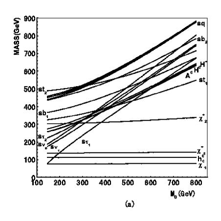
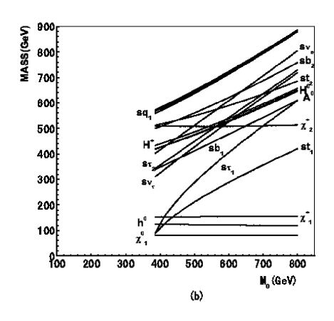
Figure 1: The mass spectrum versus $m_{0}$ for fixed $M_{1/2}$=200 Gev, $tan\beta$=40, $\delta^{d}_{23RR}$=(0.04-0.03i), and sign($\mu$)=+1 without the constraints from the low energy experiments imposed. (a) is for $A_{0}=0$. (b) is for $A_{0}$=-1000.

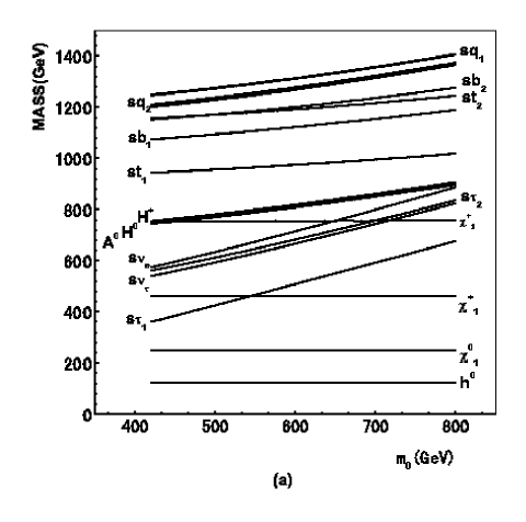
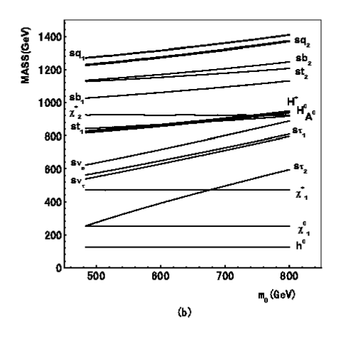
Figure 2: The mass spectrum versus $m_{0}$ for fixed $M_{1/2}$=600 Gev, $tan\beta$=40, $\delta^{d}_{23RR}$=(0.04-0.03i), and sign($\mu$)=+1 with the constraints from the low energy experiments imposed. (a) is for $A_{0}=0$. (b) is for $A_{0}$=-1000.

V Numerical analysis

In this section, we will discuss the numerical results and make an analysis.

V.1 Parameters input

Parameters in our calculation are list :

$$\begin{array}[]{ll@{\,}@{\qquad}lll}&m_{b}=4.8GeV,m_{c}=1.4GeV,&m_{s}=0.2GeV,m_{\mu}=0.1057GeV,&m_{\tau}=1.7769GeV,\\ &M_{B}=5.28GeV,M_{J/\psi}=3.10GeV,&M_{\psi^{\prime}}=3.69GeV,M_{K^{*}}=0.89GeV,&M_{K}=0.49GeV,\\ &\Gamma_{B}=4.22\times 10^{-13}GeV,&\Gamma_{J/\psi}=8.70\times 10^{-5}GeV,&\Gamma_{\psi^{\prime}}=27.70\times 10^{-5}GeV\\ &\Gamma({J/\psi}\to l^{+}l^{-})=5.26\times 10^{-6}GeV,&\Gamma({\psi^{\prime}}\to l^{+}l^{-})=2.14\times 10^{-6}GeV\end{array}$$ (56)

V.2 Constraints from experiments

In our calculation, we consider the constraints from $B\to X_{s}\gamma$, $B_{s}\to\mu^{+}\mu^{-}$, $\Delta M_{s}$, $B\to K^{(*)}l^{+}l^{-}$, and $\tau\to\mu\gamma$. The leading order $B_{s}\to X_{s}\gamma$ branching ratio normalized to $Br(B\to X_{c}e\bar{\nu})$ can be written as

$$Br(B\to X_{s}\gamma)=\frac{6\alpha_{em}}{\pi f(z)}|\frac{V_{tb}V_{ts}^{*}}{V_{cb}}|^{2}Br(B\to X_{c}e\bar{\nu})(|C_{7}(m_{b})|^{2}+|C^{\prime}_{7}(m_{b})|^{2})$$

where $\sqrt{z}=m_{c}^{pole}/m_{b}^{pole}$ , $f(z)$ is the phase space function. We take $2\times 10^{-4}<Br(B\to X_{s}\gamma)<4.5\times 10^{-4}$, considering the theoretical uncertainties. The $B\to X_{s}\gamma$ make a direct constraint on $|C_{7}(m_{b})|^{2}+|C^{\prime}_{7}(m_{b})|^{2}$. The single insertion term $\delta_{23}^{LR(RL)}$ in $C^{\prime}_{7}(m_{b})$ are more severely constrained than $\delta_{23}^{LL(RR)}$, due to the strong enhancement factor $m_{\tilde{g}}/m_{b}$ associated with single $\delta^{dLR(RL)}_{23}$ insertion term in $C^{(\prime)}_{7}(m_{b})$. Because the double insertion term $\delta^{dLL(RR)}_{23}\delta^{dLR(LR*)}_{33}$ is also enhanced by $m_{\tilde{g}}/m_{b}$, $\delta^{dLL(RR)}_{23}$ is constrained to be order of $10^{-2}$ if the left-right mixing of scalar bottom quark $\delta^{dLR(RL)}_{33}$ is large ($\sim 0.5$). Nevertheless, in the large $\tan\beta$ case the chargino contribution can destructively interfere with the SM (plus the charged Higgs) contribution so that the constraint can be easily satisfied.

The branching ratio $Br(B\to\mu^{+}\mu^{-})$ is given as wuxh

$${\rm Br}(B_{s}\rightarrow\mu^{+}\mu^{-}) = \frac{G_{F}^{2}\alpha^{2}_{\rm em}}{64\pi^{3}}m^{3}_{B_{s}}\tau_{B_{s}}f^{2}_{B_{s}}|\lambda_{t}|^{2}\sqrt{1-4\widehat{m}^{2}}[(1-4\widehat{m}^{2})|C_{Q_{1}}(m_{b})-C^{\prime}_{Q_{1}}(m_{b})|^{2}+$$ (57)

$$|C_{Q_{2}}(m_{b})-C^{\prime}_{Q_{2}}(m_{b})+2\widehat{m}(C_{10}(m_{b})-C^{\prime}_{10}(m_{b}))|^{2}]$$

where $\widehat{m}=m_{\mu}/m_{B_{s}}$. With large $C^{(\prime)}_{Q_{1,2}}$, $Br(B\to\mu^{+}\mu^{-})$ can have large enhancements bsmu . The new $D_{0}$ experimental upper bound of ${\rm Br}(B_{s}\to\mu^{+}\mu^{-})$ is $4.6\times 10^{-7}$  d0 at $90\%$ confidence level. It gives a stringent constraint on $C^{(\prime)}_{Q_{1,2}}$ and consequently the parameter space of the model. At the same time we require that predicted branching ratios of $B\to X_{s}\mu^{+}\mu^{-}$ and $B\to K^{(*)}\mu^{+}\mu^{-}$ falls within 1 $\sigma$ experimental bounds.

We also impose the current experimental lower bound $\Delta M_{s}>14.4ps^{-1}$ msd . The $\delta^{dLR(RL)}_{23}$ contribution to $\Delta M_{s}$ is small because it is constrained to be order of $10^{-2}$ by Br($B\to X_{s}\gamma$). The dominant contribution to $\Delta M_{s}$ comes from $\delta^{dLL(RR)}_{23}$ insertion with both constructive and destructive effects compared with the SM contribution, where the too large destructive effect is ruled out, because SM prediction is only slightly above the present experiment lower bound.

Furthermore, as analyzed in ref. cmsvv , there is the correlation between flavor changing squark and slepton mass insertions in SUSY GUTs. The correlation leads to a bound on $\delta_{23}^{dRR}$ from the rare decay $\tau\to\mu\gamma$. We update the analysis with latest BELLE upper bound of Br($\tau\to\mu\gamma$)$<3.1\times 10^{-7}$ taumugamma at $90\%$ confidence level in the SUSY SO(10) model.

Table 1: The Wilson coefficients for the two cases in the $SUSYSO(10)$. The SM values also are listed for comparison. The values in bracket are for $l=\tau$.

$A_{0}$	$C_{Q_{1}}$	$C_{Q_{1}}^{\prime}$	$C_{Q_{2}}$	$C_{Q_{2}}^{\prime}$
SM	0	0	0	0
$A_{0}=0$	0.074+0.I(1.252+0.001I)	-0.013+0.008I(-0.213+0.128I)	-0.075+0.I(-1.267-0.001I)	-0.013+0.008I(-0.216+0.129I)
$A_{0}=-1000$	0.106+0.I(1.775+0.002I)	-0.247+0.242I(-4.148+4.074I)	-0.107+0.I(-1.797-0.002I)	-0.250+0.246I(-4.202+4.128I)

$A_{0}$	$C_{7}^{eff}$	$C_{7}^{{}^{\prime}eff}$	$C_{9}$	$C^{\prime}_{9}$	$C_{10}$	$C^{\prime}_{10}$
SM	-0.313	0	+4.344	0	-4.669	0
$A_{0}=0$	-0.225-0.I	-0.02-0.01I	4.277+0.I	-0.-0.002I	-4.717-0.I	-0.001+0.019I
$A_{0}=-1000$	-0.219+0.I	0.039-0.038I	4.275+0.I	0.011+0.072I	-4.732-0.I	-0.075-0.670I

V.3 The Numerical results and Conclusions

We will focus on the parameter space at large $tan\beta$. The reason for this is that in the large $tan\beta$ region of parameter space the contributions of NHB exchange become very important for quark level semi-leptonic transitions $b\to sl^{+}l^{-}$ when the final state lepton is either a muon or tau dyb ; hy . In numerical calculations, we take $\tan\beta$=40, sign($\mu$)=+1, and $A_{0}=0,-1000$ and get the sparticle mass spectrum and mixing at the EW scale. Using the resulted Wilson coefficients, we calculate the IMS, FBA and polarization asymmetries of processes $B\to K^{(*)}l^{+}l^{-}$ under the constraints on $\delta_{23}^{dRR}$ from the all relevant experiments as discussed in subsection VB, whose phase varies from 0 to $2\pi$.

The Wilson coefficients $C_{Q_{1}}^{(\prime)}$ and $C_{Q_{2}}^{(\prime)}$ come from NHB exchanging. Specially, we are interested in the case of maximal enhancements of $C_{Q_{1,2}}^{(\prime)}$. Through scanning the parameter space under constraints, we find, for $A_{0}=0$, when $m_{0}$=800GeV, $M_{1/2}$=400GeV (for $A_{0}$=-1000, $M_{1/2}$=500GeV), $C_{Q_{1,2}}^{(\prime)}$ have maximal values. The obtained $C_{Q_{1,2}}^{(\prime)}$ and other relevant Wilson coefficients in the two cases and in SM are listed in Table I. From Table I, we can know: (i) the NHB contributions in the case of $A_{0}=-1000$ are larger than those in the case of $A_{0}=0$ except for $C_{9}$; (ii) the Wilson coefficients $C_{Q_{1,2}}^{\prime}$ of primed operators are dominant, which is due to the presence of $\delta_{23}^{dRR}$ of order one at the high scale in the SUSY SO(10) model, and their imaginary parts are sizable, which contribute to the normal polarization, a T violating observable.

The figures for the dependence of observable on $\hat{s}$ with and without long-distance contributions are presented in Fig.(3-7) in the case of $A_{0}=-1000$, where the solid lines denote the all contributions ($W^{\pm},H^{\pm}$, chargino, gluino, neutrilino propagated in the loop) including the NHB contributions; the dot lines present the SM contribution plus only the NHB contributions, and the dot-dashed lines are for the SM contribution. We also calculated the dependence of observable on $\hat{s}$ in the case of $A_{0}=0$ and give the results for $A_{0}=0$ when the two cases have a sizable difference.

The IMS of the process $B\to K^{(*)}l^{+}l^{-}$ is given in Fig.3, where the left two figures are for $B\to K^{(*)}\mu^{+}\mu^{-}$ and the right for $B\to K^{(*)}\tau^{+}\tau^{-}$. For the case of $B\to K\mu^{+}\mu^{-}$, we can see that, at the low $\hat{s}$ region, there are some enhancement from NHB contributions. Compared to the decay $B\to K\mu^{+}\mu^{-}$, the IMS of $B\to K^{*}\mu^{+}\mu^{-}$ deviates from the SM prediction sizably in the whole region of $\hat{s}$. Nevertheless, the SUSY effects are small compared with the SM for the decay $B\to K^{(*)}\tau^{+}\tau^{-}$.

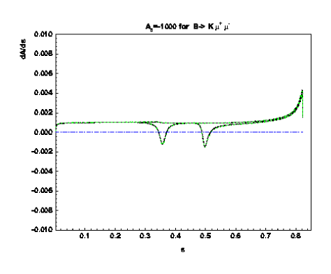
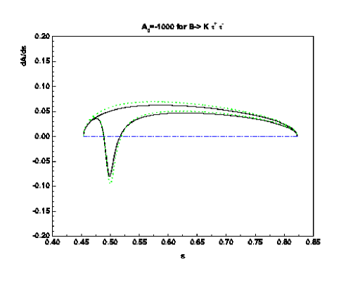
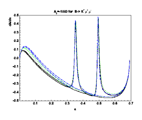
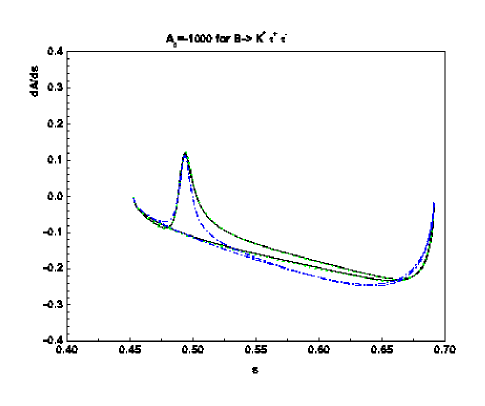
Figure 4: The FBA of the process $B\to K^{(*)}l^{+}l^{-}$ for $A_{0}=-1000$. The line conventions are the same as those in Fig. 3.

The Fig. 4 is for the FBA ($dA/d\hat{s}$) of the decay $B\to K^{(*)}l^{+}l^{-}$, where the left two figures are for $l=\mu$ and the right for $l=\tau$, like that in Fig.3. As it is known, the FBA ($dA/d\hat{s}$) of $B\to Kl^{+}l^{-}$ in the SM is zero. Since FBA arises in the SUSY models only when NHB effects are taken into account, it provides a good probe to test these effects. Our numerical results show that the average of FBA in $B\to K\mu^{+}\mu^{-}$ can reach only 0.001 which is too small to be observed. The average of FBA in $B\to K\tau^{+}\tau^{-}$ can reach -0.1 and 0.05 for the case of $A_{0}=0$ and $A_{0}=-1000$, respectively. (The reason why FBA in the two cases has the opposite sign is that the sign of function $S_{1}$ in these two cases is opposite.) So, the $10^{10}-10^{11}$ $B_{d}\;\bar{B}_{d}$ pairs per year, which is in the designed range in the future super B factors with B hadrons $10^{10}-10^{12}$ per year superb , is needed in order to observe the FBA with good accuracy. Our results show that the SUSY effects show up at the low $\hat{s}$ region for the FBA of $B\to K^{*}\mu^{+}\mu^{-}$ and the deviation from SM is 0.05 or so. It is worth to note that there is a sizable change of the position of the zero-point of the FBA in $B\to K^{*}\mu^{+}\mu^{-}$ in the SUSY SO(10) model, as it can be seen in Fig.5, which could be tested in the future experiments with high precision. For FBA in $B\to K^{*}\tau^{+}\tau^{-}$, the deviation from the SM is about several percent. The average of FBA of $B\to K^{*}\tau^{+}\tau^{-}$ can reach 0.3 in the case of $A_{0}=0$. To observe the FBA in $B\to K^{*}\tau^{+}\tau^{-}$ decay at 1$\sigma$ level, the required number of events is $1.1\times 10^{8}$. The number of B$\bar{B}$ pairs that is expected to be produced at B factories is about $N\simeq 5\times 10^{8}$. Therefore the FBA in $B\to K^{*}\tau^{+}\tau^{-}$ could be observed at B factories. Hence, with the enhancement of experimental precision and statistics, the measurements of FBA would provide more data and effectively pin to the NP effects.

Now, we turn to discuss the lepton polarization. We present the longitudinal, transverse and normal polarization in the Fig.(5,6,7) for $B\to K^{(*)}l^{+}l^{-}$ decay. As it can be seen in Fig. 5 and 6, the $dL/d\hat{s}$ of $B\to K^{(*)}\mu^{+}\mu^{-}$ is not sensitive to the NHB effects, while for $dT/d\hat{s}$ of $B\to K(K^{*})\mu^{+}\mu^{-}$, the deviation from SM can reach 0.1 (0.05). As it is expected, the contribution from the $\tau^{+}\tau^{-}$ channel is much larger than that from the $\mu^{+}\mu^{-}$ one. For $B\to K^{(*)}\tau^{+}\tau^{-}$, the NHB contributions are manifest and dominant, and both $dL/d\hat{s}$ and $dT/d\hat{s}$ are significantly different from SM. And the $dL/d\hat{s}$ of $B\to K\tau^{+}\tau^{-}$ can even reach 0.6. Thus, the NHB effects are sensitive to $B\to K^{(*)}\tau^{+}\tau^{-}$ and will be observable at B factories.

The $dN/d\hat{s}$ of $B\to K^{(*)}l^{+}l^{-}$ decay are given in Fig. 7. The average of $dN/d\hat{s}$ can reach several percent for $B\to K\mu^{+}\mu^{-}$ which could be observed in the future super B factories, while it is the order of $10^{-3}$ for $B\to K^{*}\mu^{+}\mu^{-}$ which can not be observed even in designed super B factories. The average of $dN/d\hat{s}$ in $B\to K\tau^{+}\tau^{-}$ is 0.05 or so. For $B\to K^{*}\tau^{+}\tau^{-}$, the deviation from SM is a few percent. As noted above, the Wilson coefficient $C_{10}$ is real and $C_{10}^{\prime},C_{Q_{i}}^{(\prime)}=0$ (precisely speaking, they are negligibly small) in the SM so that $dN/d\hat{s}=0$ in $B\to K\mu^{+}\mu^{-}$ in the SM. It is still true in the minimal super gravity model (mSUGRA) and SUSY models with real universal boundary conditions at the high scale 0004262 . In the SUSY SO(10) model we considered, the complex flavor non-diagonal down-type squark mass matrix element of 2nd and 3rd generations of order one at the GUT scale induces the complex couplings which lead to the complex Wilson coefficients and consequently the non zero normal polarization of $B\to K\mu^{+}\mu^{-}$. Therefore, the measurements of the CP violating (as usual, the CPT invariance is assumed in the paper) normal polarization in $B\to Kl^{+}l^{-}$ could discriminate the SUSY SO(10) model (and other SUSY models with the flavor non diagonal complex couplings) from the SM and mSUGRA.

In summary, we have carried out a study of SUSY effects, in particular, the neutral Higgs bosons contributions to the IMS, FBA and polarization, in the exclusive decay $B\to K^{(*)}l^{+}l^{-}$ ($l=\mu,\tau$) in the SUSY SO(10) model, taking account of the constraints from existing experimental data such as $b\to s\gamma$, $\Delta M_{s}$, $Br(B\to K^{(*)}\mu^{+}\mu^{-})$, $\tau\to\mu\gamma$ as well as the upper bound of $Br(B_{s}\to\mu^{+}\mu^{-})$. Our main findings can be summarized as follows:

• The IMS of the process $B\to K^{(*)}\mu^{+}\mu^{-}$ can sizably deviate from the SM.

• The FBA comes only from NHB contributions in $B\to Kl^{+}l^{-}$ and its average for $l=\mu$ is nonzero but too small to be ovserved. However for $B\to K\tau^{+}\tau^{-}$, it is the order of 10$\%$, which should be within the luminosity reach of coming B factories. The SUSY effects show up at the low $\hat{s}$ region for the FBA of $B\to K^{*}\mu^{+}\mu^{-}$ and the deviation from SM is 0.05 or so. Moreover, there is a sizable change of the position of the zero-point of the FBA in $B\to K^{*}\mu^{+}\mu^{-}$, which can be used to discriminate the model from the SM.

• The average of $dN/d\hat{s}$ can reach several percent for $B\to K\mu^{+}\mu^{-}$ and it is 0.05 or so for $B\to K\tau^{+}\tau^{-}$, which could be measured in the future super B factories and provide a useful information to probe new physics and discriminate different models.

• The longitudinal polarization, $dL/d\hat{s}$, of $B\to K^{(*)}\mu^{+}\mu^{-}$ is not sensitive to the NHB effects. However, for the transverse polarization, $dT/d\hat{s}$, of $B\to K(K^{*})\mu^{+}\mu^{-}$, the deviation from SM can reach 0.1 (0.05) which could be seen in B factories. For $B\to K^{(*)}\tau^{+}\tau^{-}$, the NHB contributions are manifest and dominant, and both $dL/d\hat{s}$ and $dT/d\hat{s}$ are significantly different from SM. And the $dL/d\hat{s}$ of $B\to K\tau^{+}\tau^{-}$ can even reach 0.6, which can be measured in B factories.

Therefore, the experimental investigation of observable, in particular, FBA and the polarization components, in the $B\to K^{(*)}l^{+}l^{-}$ decays in the present B factories and future super B factories can be used to search for SUSY effects, in particular, NHB effects, in SUSY grand unification models.

References

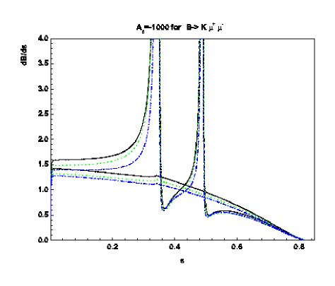
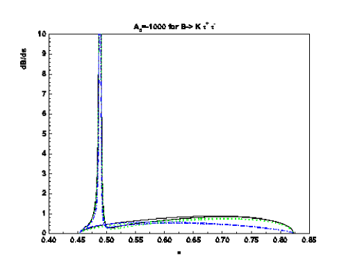
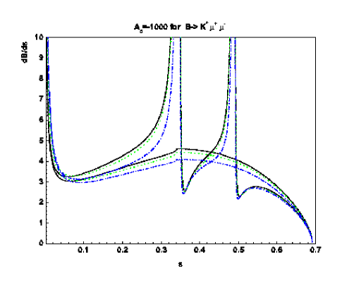
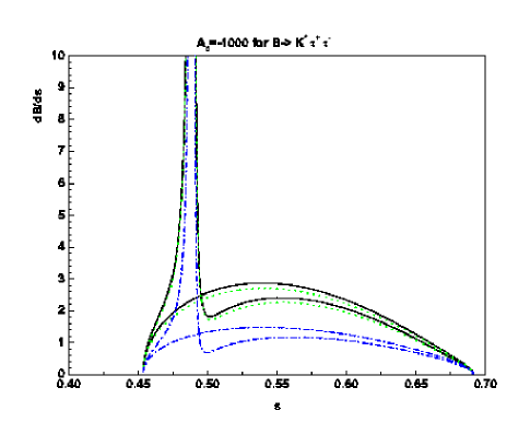
Figure 3: The IMS of the process $B\to K^{(*)}l^{+}l^{-}$ for $A_{0}=-1000$. The solid line(black), dot line(green), and dashed-dot line(blue) represent the all contributions included, the SM contributions plus only the NHB contributions, and the SM contributions, respectively. Both the total (SD+LD) and the pure SD contributions are shown in order to compare. In the fig. we write ”s” in stead of ”$\hat{s}$” for simplicity.

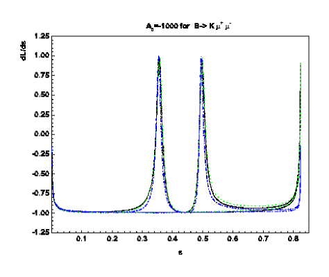
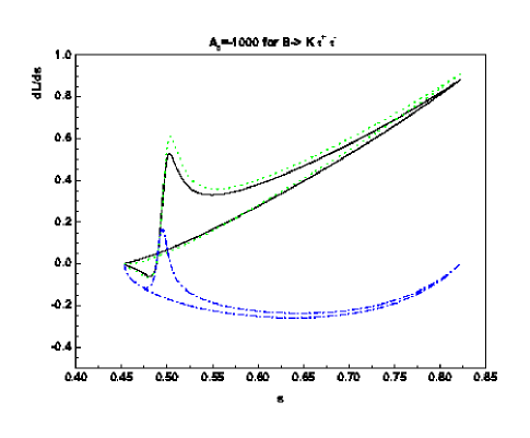
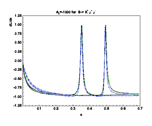
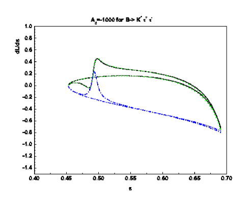
Figure 5: The $dL/d\hat{s}$ of the process $B\to K^{(*)}l^{+}l^{-}$ for $A_{0}=-1000$. The line conventions are the same as those in Fig. 3.

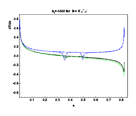
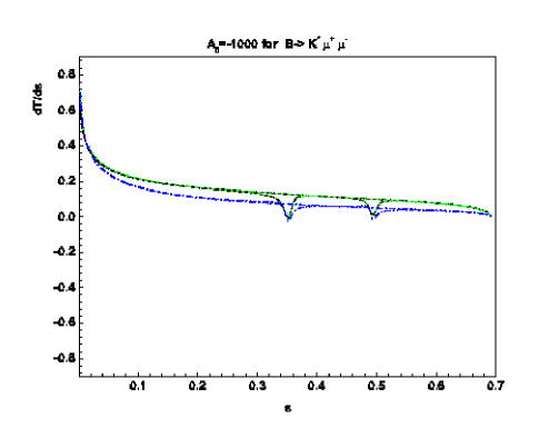
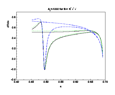
Figure 6: The $dT/d\hat{s}$ of the process $B\to K^{(*)}l^{+}l^{-}$ for $A_{0}=-1000$. The line conventions are the same as those in Fig. 3.

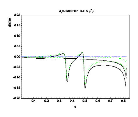
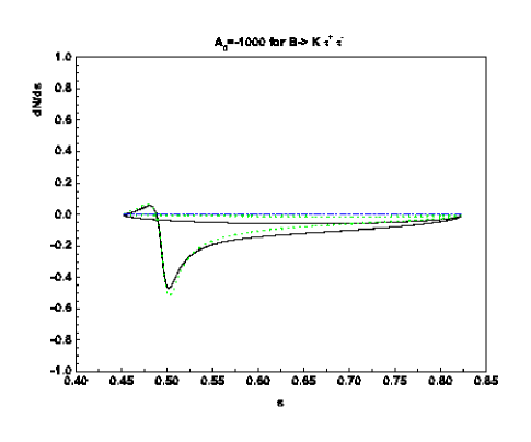
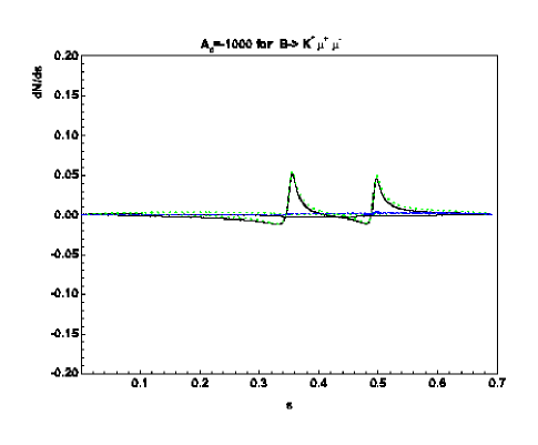
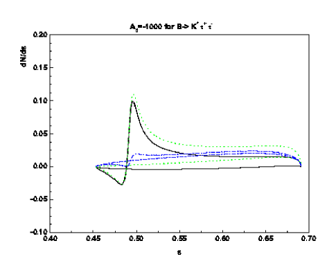
Figure 7: The $dN/d\hat{s}$ of the process $B\to K^{(*)}l^{+}l^{-}$ for $A_{0}=-1000$. The line conventions are the same as those in Fig. 3.

References

• (1) A.Ishikawa, (Belle Collaboration), Lecture given at ICHEP 2004.
• (2) A. Ishikawa et. al, BELLE Collaboration, Phys. Rev. Lett. 91, 261601 (2003); B. Aubert et al., (BABAR Collaboration), Phys. Rev. Lett. 91, 221802 (2003).
• (3) P. Ball and R. Zwicky, hep-ph/0406232; M.A. Ivanov and V.E. Lyubovitskij, Lectures given at International School on Heavy Quark Physics, Dubna, Russia, 27 May - 5 Jun 2002; W. Jaus and D. Wyler, Phys. Rev. D 41 (1990) 3405; P. Colangelo et al., Phys. Lett. B317 (1993) 183; Ceng et al., Phys. Rev. D 54 (1996) 3656; Amand Faessler et al., EPJ C, 4, C18, 1 C33 (2002).
• (4) P. Colangelo et al., Phys. Rev. D 53 (1996) 3672 [arXiv:hep-ph/9510403]; Erratum, ibid, D 57 (1998) 3186.
• (5) I.I. Balitsky, V.M. Braun and A.V. Kolesnichenko, Nucl. Phys. B312 (1989) 509; V.L. Chernyak and I.R. Zhitnitsky, Nucl. Phys. B345 (1990) 137; V.M. Braun, Preprint NORDITA C98 C1 CP [arXiv:hep-ph/9801222]; A. Khodjamirian and R. Ruckl, [arXiv:hep-ph/9801443]; P. Ball and V.M. Braun, Phys. Rev. D 58 (1998) 094016 [arXiv:hep-ph/9805422]; Nucl. Phys. B543 (1999) 201 [arXiv:hep-ph/9810475]; P. Ball et al., Nucl. Phys. B529 (1998) 323 [arXiv:hep-ph/9802299]; P. Ball, JHEP 09 (1998) 005 [arXiv:hep-ph/9802394]; JHEP 01 (1999) 010 [arXiv:hep-ph/9812375].
• (6) C.Q. Geng and C.P. Kao, Phys. Rev. D 54 (1996) 5636 [arXiv:hep-ph/9608466]; Phys. Rev. D 57 (1998) 4479.
• (7) S. Fukaea, C.S. Kimb, T. Morozumi, and T. Yoshikawac, Phys. Rev. D 59 (1999) 074013 [arXiv:hep-ph/9807254]; T.M. Aliev,C. S. Kim and Y. G. Kim, Phys. Rev. D 62, 014026 (2000) [arXiv:hep-ph/9910501]; T. M. Aliev,et.al, Nucl. Phys. B607 (2001) 305-325 [arXiv:hep-ph/0009133]; T.M. Aliev, M.K. Cakmak, A. $\ddot{O}$zpineci, M. Savci, Phys. Rev. D 64 (2001) 055007 [arXiv:hep-ph/0103039].
• (8) Benjamin Grinstein, Dan Pirjol,CTP-MIT-3490,[arXiv:hep-ph/0404250].
• (9) T.M. Aliev, M. Savci, Phys. Lett. B481 (2000) 275-286 [arXiv:hep-ph/0003188].
• (10) L.T. Handoko, C.S. Kim, T. Yoshikawa, Phys. Rev. D 65 (2002) 077506 [arXiv:hep-ph/0112149].
• (11) A. Ali, E. Lunghi, C. Greub, G. Hiller, DESY 01-217, BUTP-01-21, SLAC-PUB-9076 [arXiv:hep-ph/0112300].
• (12) T.M. Aliev, M. Savci, A. Ozpineci, H. Koru,J.Phys. G24 (1998) 49-65 [arXiv:hep-ph/9705222].
• (13) Qi-Shu Yan, Chao-Shang Huang, Liao Wei, Shou-Hua Zhu, Phys. Rev. D 62 (2000) 094023 [arXiv:hep-ph/0004262].
• (14) A. Ali, P. Ball, L.T. Handoko, G. Hiller, Phys. Rev. D 61 (2000) 074024 [arXiv:hep-ph/9910221].
• (15) F. Kr$\ddot{u}$ger, E. Lunghi, Phys. Rev. D 63 (2001) 014013 [arXiv:hep-ph/0008210].
• (16) C.S. Huang, Nucl.Phys. Proc. Suppl. 93 (2001) 73-78 [arXiv:hep-ph/0009149]; C. Bobeth, T. Ewerth, F. Kruger, J. Urban, Phys. Rev. D 64 (2001) 074014 [arXiv:hep-ph/0104284].
• (17) Guray Erkol, Gursevil Turan, Nucl. Phys. B635 (2002) 286-308 [arXiv:hep-ph/0204219].
• (18) S. R. Choudhury et al., Phys. Rev. D 69 (2004) 054018 [arXiv:hep-ph/0307276].
• (19) S. Rai Choudhury et al., Phys. Rev. D 68, 054016 (2003) [arXiv:hep-ph/0304084]
• (20) Wafia Bensalam, David London, Nita Sinha, Rahul Sinha, Phys. Rev. D 67 (2003) 034007 [arXiv:hep-ph/0209228]
• (21) T.M. Aliev, V. Bashiry, M. Savci, Eur. Phys. J. C35 (2004) 197-206 [arXiv:hep-ph/0311294]; JHEP 0405 (2004) 037 [arXiv:hep-ph/0403282]; A.S. Cornell, Naveen Gaur, [arXiv:hep-ph/0408164].
• (22) V. Barger et al., Phys. Rev. Lett. 82 (1999) 2640 [arXiv:astro-ph/9810121]; E. lisi et al., Phys. Rev. Lett. 85 (2000) 1166 [arXiv:hep-ph/0002053]; John N. Bahcall et al., Phys. Rev. Lett. 90, 131301 (2003) [arXiv:astro-ph/0212331]; John N. Bahcall and M. H. Pinsonneault, Phys. Rev. Lett. 92, 121301 (2004) [arXiv:astro-ph/0402114]; Sandhya Choubey and Probir Roy, Phys. Rev. Lett. 93, 021803 (2004) [arXiv:hep-ph/0310316].
• (23) K.S. Babu and S.M. Barr, Phys. Lett. B381 (1996) 202 [arXiv:hep-ph/9511446]; C.H. Albright, K.S. Babu, and S.M. Barr, Phys. Rev. Lett. 81 (1998) 1167 [arXiv:hep-ph/9802314]; J. Sato and T. Yanagida, Phys. Lett. B430 (1998) 127 [arXiv:hep-ph/9710516]; N. Irges, S. Lavignac, and P. Ramond, Phys. Rev. D 58 (1998) 035003 [arXiv:hep-ph/9802334].
• (24) Mu-Chun Chen, K.T. Mahanthappa,Phys.Rev.D62 113007 (2000), [arXiv:hep-ph/0005292].
• (25) D. Chang, A. Masiero and H. Murayama, Phys. Rev. D67 (2003) 075013 [arXiv:hep-ph/0205111].
• (26) B. Bajc, G. Senjanovi$\acute{c}$ and F. Vissani, [arXiv:hep-ph/0210207]; H.S. Goh, R.N. Mohapatra and S.-P. Ng, [arXiv:hep-ph/0303055].
• (27) X-J. Bi, Y-B. Dai and X-Y Qi, Phys. Rev. D63 096008 (2001); X-J. Bi and Y-B. Dai, Phys. Rev. D66 076006 (2002).
• (28) Mu-Chun Chen, K.T. Mahanthappa, Phys.Rev.D65 053010 (2002), [arXiv:hep-ph/0106093]; Mu-Chun Chen, K.T. Mahanthappa,Phys.Rev.D68 017301 (2003),[arXiv:hep-ph/0212375];Mu-Chun Chen and K.T. Mahanthappa, Int.J.Mod.Phys. A18:5819-5888,2003 [arXiv:hep-ph/0305088];Mu-Chun Chen, K.T. Mahanthappa,[arXiv:hep-ph/0409096].
• (29) Sebastian Jager, Ulrich Nierste,FERMILAB-Conf-03/394-T, [arXiv:hep-ph/0312145].
• (30) Y-B. Dai, C-S. Huang, W-J. Li, X-H. Wu, [arXiv:hep-ph/0407263].
• (31) T. Goto et al., Phys. Rev. D 55 (1997) 4273; T. Goto, Y. Okada and Y. Shimizu, Phys. Rev. D 58 (1998) 094006; S. Bertolini, F. Borzynatu, A. Masiero and G. Ridolfi, Nucl. Phys. B353 (91) 591.
• (32) Y-B. Dai, C-S. Huang, H-W. Huang, Phys. Lett. B390:257-262,1997; Erratum-ibid. B513:429-430, 2001 [arXiv:hep-ph/9607389].
• (33) Chao-Shang Huang, Xiao-Hong Wu, Nucl. Phys. B657 (2003) 304-332 [arXiv:hep-ph/0212220]; Jian-Feng Cheng, Chao-Shang Huang, Xiao-Hong Wu, hep-ph/0404055, to appear in Nucl. Phys. B.
• (34) A.J. Buras, M. Muenz, Phys. Rev. D 52 (1995) 186-195 [arXiv:hep-ph/9501281].
• (35) D. Acosta et al., (CDF Collaboration), [arXiv:hep-ex/0403032].
• (36) C.-S. Huang, W. Liao, Q.-S. Yan, S.-H. Zhu, Phys. Rev. D63 (2001) 114021; ibid. 64 (2001) 059902(E) [arXiv:hep-ph/0006250]; For review papers, see, e.g., C.-S. Huang, Nucl. Phys. Proc. Suppl. 115, 89 (2003); A. Dedes, Mod. Phys. Lett. A18, 2627 (2003) [arXiv:hep-ph/0309233].
• (37) The $D_{0}$ collaboration, $D_{0}$ Coneference Note 4514.
• (38) A. Stocchi, Nucl. Phys. Proc. Suppl. 117(2003) 145 [arXiv:hep-ph/0211245].
• (39) A. Kagan, [arXiv:hep-ph/9806266]; T.E. Coan et al., (CLEO Collaboration), Phys. Rev. Lett. 80, 1150 (1998) [arXiv:hep-ex/9710028].
• (40) K. Hagiwara et al., Phys. Rev. D66, 010001 (2002).
• (41) M. Ciuchini et al., Phys. Rev. Lett. 92 (2004) 071801.
• (42) K.Abe et. al., Belle collaboration, Phys. Rev. Lett. 92 (2004) 171802 [arXiv:hep-ex/0310029].
• (43) T.E. Browder and A. Soni, hep-ph/0410192, and references therein.
• (44) J.L. Lopez, D.V. Nanopoulos, X. Wang and A. Zichichi, Phys. Rev. D51, 147 (1995) [arXiv:hep-ph/9406427].
• (45) C.-S. Huang and Q.-S. Yan, Phys. Lett. B442(1998) 209 [arXiv:hep-ph/9803366]; C.-S. Huang, W. Liao, and Q.-S. Yan, Phys. Rev. D59 (1999) 011701 [arXiv:hep-ph/9803460].
• (46) A. Stocchi, Nucl. Phys. Proc. Suppl. 117 (2003) 145 [arXiv:hep-ph/0211245].
Refer to caption
Refer to caption
Refer to caption
Refer to caption