Are There Diquarks in the Nucleon?

Abstract

This work is devoted to the study of diquark correlations inside the nucleon. We analyze some matrix elements which encode information about the non-perturbative forces, in different color anti-triplet diquark channels. We suggest a lattice calculation to check the quark-diquark picture and clarify the role of instanton-mediated interactions. We study in detail the physical properties of the $0^{+}$ diquark, using the Random Instanton Liquid Model. We find that instanton forces are sufficiently strong to form a diquark bound-state, with a mass of $\sim~{}500$ MeV, which is compatible with earlier estimates. We also compute its electro-magnetic form factor and find that the diquark is a broad object, with a size comparable with that of the proton.

I Introduction

A complete description of the strong interaction between quarks is available only at asymptotically short distances, where the QCD becomes weakly coupled. At the perturbative level, it is well known that two quarks strongly attract each other if they are in a $J^{P}=0^{+}$ and color anti-triplet state ptdiquark1 ; ptdiquark2 . The question whether a particularly strong attraction in this channel is present also at intermediate and large distances -where the theory is strongly coupled- has long been debated. From a phenomenological point of view, the notion of strongly correlated, quasi-bound diquarks has been widely used to describe low-$q^{2}$ processes in hadrons ( for early studies see earlydiquarks1 , for a review see earlydiquarks2 , for further references see also earlydiquarks3 ). For example, it has been observed that the anti-triplet scalar diquarks play an important role in non-leptonic weak decays of both hyperons and kaons stech ; stech2 ; delta12 .

The problem of understanding the role of diquark correlations in QCD has recently become particularly important, after several experimental groups have reported evidence for the first truly exotic state, the $\Theta^{+}$ pentaquark exppropentaquark . The existence of such a state was originally predicted by Diakonov, Petrov and Polyakov using a soliton model pentaquark and several experiments are being performed to confirm this important discovery. There are also on-going theoretical inverstigations based on lattice QCD simulations (see for example saza and references therein).

The claims of the observation of the pentaquark have triggered a huge theoretical activity, aiming to identify possible dynamical mechanisms which could explain the existence and the extremely narrow width of this resonance. Jaffe and Wilczek jw have suggested that several important properties of the hadronic spectrum, including the existence of a pentaquark anti-decuplet, could be explained by assuming that the non-perturbative quark-quark interaction is particularly attractive in the anti-triplet $0^{+}$ channel, leading to strongly correlated scalar $u-d$ diquarks, inside hadrons.

The implications of the diquark hypothesis on the structure and the decay of the pentaquark has been analyzed in a number of recent works (for an incomplete list see incomplete ). At the same time, the Jaffe-Wilczek analysis has opened a related discussion concerning the possible non-perturbative mechanisms in QCD, which can lead to a strong attraction in the scalar anti-triplet channel. Shuryak and Zahed have performed an analysis of the hadronic spectrum assuming that diquark correlations are induced by instantons diquarkSHU . In addition to diquarks, Kochelev, Lee and Vento have also suggested the existence of instanton-induced tri-quarks diquarkVENT . It should be mentioned all models in which the quarks in the pentaquark are strongly correlated contrast with the original mean-field picture proposed by Diakonov, Petrov and Polyakov, in which two-body correlations are neglected pentaquark .

Even though the experimental evidence for the $\Theta^{+}$ pentaquark is still a matter of debate, understanding if strong correlations in the $0^{+}$ anti-triplet diquark channel are present in the vacuum and in hadrons is an important open problem in QCD. At present, Lattice Gauge Theory represents the only available framework to perform ab-initio non-perturbative calculations in QCD. It is therefore natural to attempt to use it to address this fundamental question. In this paper, we take a first step in this direction. We identify and study a set of lattice-calculable matrix-elements, which are very sensitive to the quark-quark interaction in different diquark channels. In order to show that these matrix elements can be used to gain insight on diquark correlations inside hadrons, we compute them using three different phenomenological models: a naive $SU(6)$ Non-Relativistic Quark Model, in which dynamical diquark correlations are absent, the Random Instanton Liquid Model, where scalar diquarks are strongly favored by the ’t Hooft interaction, and a Chiral Soliton Model, where the ’t Hooft interaction is treated at the mean-field level. We show that these models lead to very different predictions. We also identify a lattice calculation which can check if the strong attraction in the scalar anti-triplet diquark channel can be mediated by instantons, as in the model of Shuryak and Zahed.

In the second part of this work, we study the physical properties of the diquarks induced by instanton-mediated forces. We provide unambiguous evidence that the ’t Hooft interaction leads to a $0^{+}$ bound-state of about 500 MeV. This result agrees with the early estimate by Shuryak and collaborators baryonRILM . We also compute the electro-magnetic form factor of such a bound-state, finding that its size is comparable with that of the proton. This result suggests that diquarks cannot at all be modeled as point-like objects.

The paper is organized as follows. In section II, we define the relevant matrix elements and explain why these quantities can be used to study diquark correlations, in different diquark channels. The matrix elements are computed in different models in section III and the results are analyzed in section IV. The diquark mass and size are computed in the Random Instanton Liquid Model, in section V. All the results and the conclusions of this work are summarized in section VI.

II Diquark densities in the proton

Much of the theoretical studies of the internal structure of hadrons focus on observables related to one-body local operators. These matrix elements allow to access information on the hadron internal wave-function, but are only indirectly sensitive to the Dirac and flavor structure of the non-perturbative quark-quark interaction. For example, models of the proton with drastically different diquark content typically give comparable charge radii.

Much more direct insight on quark-quark correlations inside hadrons can be learned by focusing on two-body local density operators, which simultaneously probe the position and the discrete quantum numbers of two quarks. In this view, we consider a set of four-field operators (which we shall refer to as diquark densities), in which two quarks with quantum numbers of a scalar, vector, axial-vector and pseudo-scalar color anti-triplet diquark are destroyed and re-emitted, in the same point.

We work with Euclidean space-time, and we define:

$$D_{\Gamma}({\bf r}) = F_{\Gamma}^{a\,\dagger}({\bf r},0)F^{a}_{\Gamma}({\bf r},0),$$ (1)

$$F^{a}_{\Gamma}(x) = \epsilon^{abc}u^{b}(x)\,C\,\Gamma\,d^{c}(x),$$ (2)

where $C=i\,\gamma_{2}\,\gamma_{4}$ is the charge-conjugation operator, $\Gamma\in\{1,\gamma_{5},\gamma_{\mu},\gamma_{\mu}~{}\gamma_{5},\sigma_{\mu,\nu}\}$ and $a,b,c$ are color indexes The operator $F^{a}_{\Gamma}(x)$ absorbs two quarks in a point with quantum numbers of a color anti-triplet diquark. For example, $F^{a}_{\gamma_{3}}(x)$ annihilates an axial-vector diquark, while $F^{a}_{\gamma_{5}}(x)$ absorbs scalar diquarks. Hence, the matrix element:

$$\rho_{\Gamma}({\bf r})=\langle P|D_{\Gamma}({\bf r})|P\rangle$$ (3)

measures the probability amplitude to find at time $t=0$ two quarks at the point ${\bf r}$ in the proton, in a anti-triplet color state and with quantum numbers specified by $\Gamma$.

The choice of $\Gamma$ in (2) determines the transformation property of the $F_{\Gamma}^{a}(x)$ operator under exchanges of the flavor indexes. Acting on the vacuum, the operator $F_{\Gamma}^{a\,\dagger}\left({\bf r},0\right)$ creates at time $t=0$ the diquark state:

$$F_{\Gamma}^{a\,\dagger}\left({\bf r},0\right)\left|0\right\rangle=\varepsilon^{abc}\left(\Gamma^{\dagger}C\right)_{s\,t}\left|{\bf r}\,s\,d\,b;{\bf r}\,t\,u\,c\right\rangle,$$ (4)

where $s,t$ are spinor indexes, $a,b,c$ are color indexes, $u,d$ are quark flavors. This state is symmetric under the exchange of the coordinates ${\bf r}$ and antisymmetric under the exchange of color. Under the exchange of the Dirac indexes, the state is either symmetric or anti-symmetric, depending on $\Gamma$, as shown in table 1:

$\Gamma$	space	Dirac	flavor	color	total
$1$	S	A	A $\left(T=0\right)$	A	A
$\gamma_{5}$	S	A	A $\left(T=0\right)$	A	A
$\gamma^{4}$	S	S	$S\left(T=1,M_{T}=0\right)$	A	A
$\gamma^{3}$	S	S	S $\left(T=1,M_{T}=0\right)$	A	A
$\gamma^{4}\gamma^{5}$	S	A	A $\left(T=0\right)$	A	A

Table 1: Symmetry properties of the operators $F^{a}_{\Gamma}(x)$, under exchange of space, color, flavor and Dirac indexes.

for $\Gamma=\gamma_{5}$, the matrix $\Gamma^{\dagger}C$ is antisymmetric and the diquark state is thus antisymmetric under the exchange of Dirac indexes. The state is symmetric under the exchange of space indexes and antisymmetric under the exchange of color indexes. It is by construction antisymmetric with respect to the exchange of all indexes (space, Dirac, flavor and color) so that it is necessarily antisymmetric with respect to flavor indexes, meaning that it is a flavor $T=0$ state. However, when $\Gamma=\gamma_{4}$ ( a symmetric matrix ) the diquark state is symmetric under the exchange of Dirac indexes. The state is thus necessarily symmetric with respect to flavor indexes, meaning that it is a flavor $T=1$ $M_{T}=0$ state.

The comparison of the different matrix elements (3) can provide useful insight into the internal dynamics of the hadron, in particular about the strength and the spin- and flavor- structure of the quark-quark interaction. In general, we expect that the stronger are the two-body correlations inside the hadron, the larger are the discrepancies between a mean-field description and the exact calculation. More specifically, if the quark-quark interaction is particularly attractive in the scalar anti-triplet diquark channel $-$ as it is assumed in the Jaffe-Wilczek picture $-$ then we expect that the scalar diquark density $\rho_{\gamma_{5}}({\bf r})$ should be enhanced with respect to a model in which the interaction is not particularly attractive, in this channel. In fact, the $u$ and $d$ quarks would have a larger probability “to be found” in the same point and be destroyed by the local operator $F_{\gamma_{5}}^{a}(x)$.

The diquark densities can also be used to study relativistic effects in the hadron. The $F^{a}_{1}(x)$ and $F^{a}_{\gamma_{4}}(x)$ operators mix upper and lower spinor components of the quark fields and vanish in the non-relativistic limit. Hence the densities $\rho_{1}({\bf r})$ and $\rho_{\gamma_{4}}({\bf r})$ are sensitive only to the relativistic components of the wave-function. On the contrary the operators $F^{a}_{\gamma_{3}}(x)$, $F^{a}_{\gamma_{5}\gamma_{4}}(x)$, and $F^{a}_{\gamma_{5}}(x)$ remain finite in the non-relativistic limit.

III Diquark densities in different models

In this section, we compute the predictions for the diquark densities defined in the previous section, using the Chiral Soliton Model, the $SU(6)$ Non-Relativistic Quark Model, and the Random Instanton Liquid Model. The Non-Relativistic Quark Model is used to mimic a scenario in which the quarks are very weakly dynamically correlated and do not form bound diquarks. In such a model, all spin-flavor correlations are due to the $SU(6)$ symmetry properties of the wave-function only. The Random Instanton Liquid Model calculation represents the opposite scenario, in which the non-perturbative interaction is spin-flavor dependent and is particularly attractive in the $0^{+}$ anti-triplet diquark channel. The mean-field Chiral Soliton Model can be used to mimic a scenario in which the same interaction binds the nucleon, but leads to negligible two-body correlations.

The reader who is not interested in the technical details of these calculations may skip the remaining part of this section and consider directly the discussion of the results presented in section IV.

III.1 Chiral Soliton Model

The Chiral Soliton Model (for a detailed discussion we refer the reader to e.g. chiralsoliton ; Ripka ) can be used to account for the ’t Hooft interaction in the nucleon to all orders, keeping only the leading terms in the $1/N_{c}$ expansion. Hence, in the large $N_{c}$ limit, the Random Instanton Liquid Model and Chiral Soliton Model should give similar results.

As all mean-field approaches, the Chiral Soliton Model is most efficient for calculations of matrix elements of one-body operators. Indeed, the Random Instanton Liquid Model and Chiral Soliton Model give similar predictions for the proton form factors solitonFF ; myformfactors . On the other hand, if the instanton-induced two-body correlations are strong for $N_{c}=3$, then we expect that the Random Instanton Liquid Model and the Chiral Soliton Model should give significantly different results for matrix elements of two-body operators, such as the diquark densities (3).

For $N_{f}=2$, the Chiral Soliton Model is derived by bosonization of the four-field ’t Hooft contact interaction, introducing an auxiliary chiral field. The chirally-invariant Hamiltonian governing the dynamics of the quarks field $\psi$ and the chiral fields $\sigma$ and $\pi_{a}$ ($a=1,2,3$) is:

$${\mathcal{H}}=\int d^{3}{\bf r}~{}\psi^{\dagger}\left[{\bf\alpha}\cdot{\bf p}+g\beta(\sigma+i\gamma_{5}{\bf\pi}\cdot{\bf\tau})\right]\psi$$

$$+\int d^{3}{\bf r}\left[\frac{1}{2}(\nabla\sigma)^{2}+\frac{1}{2}(\nabla{\bf\pi})^{2}+\lambda(\sigma^{2}+{\bf\pi}^{2}-\sigma_{0}^{2})^{2}\right],$$ (5)

where $\tau_{a}$ are isospin Pauli matrices, $g$ and $\lambda$ are coupling constants and $\sigma_{0}$ is the vacuum expectation value of the scalar field $\sigma$. In the large $N_{c}$ limit, one can apply the zero-loop approximation and treat the ($\sigma,{\bf\pi}$) fields as classical.

The Hamiltonian (III.1) is quadratic in the quark fields and gives rise to the single-particle Dirac equation

$$\left[-i\,{\bf\alpha\cdot\nabla}+\beta(\phi+i\gamma_{5}{\bf\chi}\cdot{\bf\tau})\right]|\lambda\rangle=\epsilon_{\lambda}|\lambda\rangle,$$ (6)

where, for convenience, we have introduced dimensionless distances and fields defined as:

$${\bf x}=g\,\sigma_{0}{\bf r},\qquad\phi=\frac{\sigma}{\sigma_{0}},\qquad\chi_{a}=\frac{\pi_{a}}{\sigma_{0}}.$$ (7)

The total energy, when $N_{c}$ quarks are accommodated in the ${\bf J}+{\bf I}={\bf 0}$ valence orbital of energy $\epsilon_{\lambda}$, is

$$E=N_{c}\,g\,\sigma_{0}~{}\epsilon_{\lambda}+\frac{\sigma_{0}}{2g}~{}\int d^{3}~{}{\bf x}\left[(\nabla\phi)^{2}+(\nabla\chi)^{2}+\frac{\lambda}{g^{4}}(\phi^{2}+{\bf\chi}^{2}-1)^{2}\right].$$ (8)

By requiring that the total energy must be stationary with respect to infinitesimal variations of the chiral fields one obtains the equations:

$$\frac{-1}{g^{2}}\,\nabla^{2}\phi+4\frac{\lambda}{g^{4}}\phi~{}(\phi^{2}+{\bf\chi}^{2}-1)+N_{c}\langle\lambda|{\bf x}\rangle~{}\beta~{}\langle{\bf x}|\lambda\rangle=0,$$ (9)

$$\frac{-1}{g^{2}}\,\nabla^{2}\chi_{a}+4\frac{\lambda}{g^{4}}\chi_{a}~{}(\phi^{2}+{\bf\chi}^{2}-1)+N_{c}\langle\lambda|{\bf x}\rangle~{}i\beta\,\gamma_{5}~{}\langle{\bf x}|\lambda\rangle=0,$$ (10)

Eq.s (6), (9) and (10) represent a self-consistent set of equations for the quark orbitals $|\lambda\rangle$ and the classical chiral fields. The chiral soliton state is a solution of such equations, in which the chiral fields are assumed to be time-independent and have a hedgehog shape:

$$\phi(x)=\phi({\bf x}),\qquad\chi_{a}(x)=\hat{{\bf x}}_{a}\chi({\bf x}).$$ (11)

In the chiral soliton model of Diakonov and Petrov chiralsoliton , the fields $\sigma$ and $\pi_{a}$ are restricted to the chiral circle, $\sigma^{2}+{\bf\pi}^{2}=\sigma_{0}^{2}$. With the ansatz (11), the Dirac equation (6) generates a bound-state composed of valence and Dirac-sea quarks:

$$|\Phi\rangle=\prod_{\mu\in valence}~{}a^{\dagger}_{\mu}~{}\prod_{\lambda\in sea}a^{\dagger}_{\lambda}~{}|0\rangle.$$ (12)

The first product of creation operators excites three valence quarks of different colors in a $s$-state wave-function in the form:

$$\langle{\bf x}~{}u|\lambda\rangle=\frac{1}{\sqrt{2}}\left(\begin{array}[]{c}i\frac{F({\bf x)}}{|{\bf x}|}~{}|\downarrow~{}\rangle\\ -\frac{G({\bf x})}{|{\bf x}|}{\bf\sigma\cdot\hat{x}}~{}|\downarrow~{}\rangle\end{array}\right),\qquad\langle{\bf x}~{}d|\lambda\rangle=\frac{1}{\sqrt{2}}\left(\begin{array}[]{c}-i\frac{F({\bf x)}}{|{\bf x}|}~{}|\uparrow~{}\rangle\\ \frac{G({\bf x})}{|{\bf x}|}{\bf\sigma\cdot\hat{x}}~{}|\uparrow~{}\rangle\end{array}\right)$$ (17)

The radial functions $F({\bf x})$ and $G({\bf x})$ are normalized according to

$$\int_{0}^{\infty}d^{3}{\bf x}~{}[~{}F^{2}({\bf x})+G^{2}({\bf x})~{}]=1,$$ (18)

and can be computed numerically.

The second product of creation operators in (11) generates the contribution of quarks in the Dirac sea. In this work, we shall neglect such a contribution and retain only the valence part of the soliton wave-function.

After having solved for the valence component of the soliton wave-function $|\Phi\rangle$, it is straightforward to compute the different diquark densities:

$$\rho_{\Gamma}\left({\bf r}\right)=\left\langle\Phi\left|\,F_{\Gamma}^{a\,\dagger}\left({\bf r},0\right)F_{\Gamma}^{a}\left({\bf r},0\right)\right|\Phi\right\rangle,\qquad\Gamma=1,i\gamma_{5},\gamma_{4},\gamma_{3},\gamma_{4}\gamma_{5}.$$ (19)

We begin by contracting the color index $a$. The diquark density becomes:

$$\rho_{\Gamma}\left({\bf r}\right)=\left(\Gamma C\right)_{s_{1}s_{2}}\left(C\Gamma\right)_{s_{3}s_{4}}\left\langle\Phi\left|d_{s_{1}}^{c_{3}\,\dagger}u_{s_{2}}^{c_{2}\,\dagger}u_{s_{3}}^{c_{2}}d_{s_{4}}^{c_{3}}-d_{s_{1}}^{c_{3}\,\dagger}u_{s_{2}}^{c_{2}\,\dagger}u_{s_{3}}^{c_{3}}d_{s_{4}}^{c_{2}}\right|\Phi\right\rangle,$$ (20)

where $s_{1},s_{2},s_{4},s_{4}=1,..,4$ are Dirac indexes and $c_{2},c_{3}=1,...,3$ are color indexes. By applying Wick’s theorem we get:

$$\left\langle\Phi\left|d_{s_{1}}^{c_{3}\,\dagger}u_{s_{2}}^{c_{2}\,\dagger}u_{s_{3}}^{c_{2}}d_{s_{4}}^{c_{3}}-d_{s_{1}}^{c_{3}\,\dagger}u_{s_{2}}^{c_{2}\,\dagger}u_{s_{3}}^{c_{3}}d_{s_{4}}^{c_{2}}\right|\Phi\right\rangle=$$ (21)

$$= N_{c}^{2}\sum_{\lambda\mu\in D}\left\langle\lambda\left|{\bf x}s_{1}d\right.\right\rangle\left\langle{\bf x}s_{4}d\left|\lambda\right.\right\rangle\left\langle\mu\left|{\bf x}s_{2}u\right.\right\rangle\left\langle{\bf x}s_{3}u\left|\mu\right.\right\rangle$$

$$+ N_{c}^{2}\sum_{\lambda\mu\in D}\left\langle\lambda\left|{\bf x}s_{1}d\right.\right\rangle\left\langle{\bf x}s_{3}u\left|\lambda\right.\right\rangle\left\langle\mu\left|{\bf x}s_{2}u\right.\right\rangle\left\langle{\bf x}s_{4}d\left|\mu\right.\right\rangle$$

$$- N_{c}\sum_{\lambda\mu\in D}\left\langle\lambda\left|{\bf x}s_{1}d\right.\right\rangle\left\langle{\bf x}s_{3}u\left|\lambda\right.\right\rangle\left\langle\mu\left|{\bf x}s_{2}u\right.\right\rangle\left\langle{\bf x}s_{4}d\left|\mu\right.\right\rangle$$

$$- N_{c}\sum_{\lambda\mu\in D}\left\langle\lambda\left|{\bf x}s_{1}d\right.\right\rangle\left\langle{\bf x}s_{4}d\left|\lambda\right.\right\rangle\left\langle\mu\left|{\bf x}s_{2}u\right.\right\rangle\left\langle{\bf x}s_{3}u\left|\mu\right.\right\rangle.$$

Substituting the explicit expression for the valence orbits (17), and performing the summation over the spinor indexes, it is straightforward to obtain the result (choosing ${\bf x}$ along the $\hat{z}$ direction):

$$\rho_{1}({\bf r}) = 0,$$ (22)

$$\rho_{\gamma_{5}}({\bf r}) = N_{c}(N_{c}-1)\left(\frac{F^{2}(g\,\sigma_{0}\,{\bf r})+G^{2}(g\,\sigma_{0}\,{\bf r})}{\sqrt{2}\,(g\,\sigma_{0}\,{\bf r})^{2}}\right)^{2},$$ (23)

$$\rho_{\gamma_{4}}({\bf r}) = 2N_{c}(N_{c}-1)\left(\frac{F(g\,\sigma_{0}\,{\bf r})~{}G(g\,\sigma_{0}\,{\bf r})}{(g\,\sigma_{0}\,{\bf r})^{2}}\right)^{2},$$ (24)

$$\rho_{\gamma_{3}}({\bf r}) = N_{c}(N_{c}-1)\left(\frac{F^{2}(g\,\sigma_{0}\,{\bf r})-G^{2}(g\,\sigma_{0}\,{\bf r})}{\sqrt{2}\,(g\,\sigma_{0}\,{\bf r})^{2}}\right)^{2},$$ (25)

$$\rho_{\gamma_{4}\gamma_{5}}({\bf r}) = N_{c}(N_{c}-1)\left(\frac{F^{2}(g\,\sigma_{0}\,{\bf r})-G^{2}(g\,\sigma_{0}\,{\bf r})}{\sqrt{2}\,(g\,\sigma_{0}\,{\bf r})^{2}}\right)^{2},$$ (26)

where we have used the relationship between ${\bf x}$ and ${\bf r}$ given by (7).

These results correspond to the different diquark densities in the soliton state, which is neither an eigenstate of the angular momentum nor an eigenstate of the isospin operator. Instead, it is characterized by its (vanishing) eigenvalue of the grand-spin ${\bf G}={\bf J}+{\bf I}$ operator. In order to make contact with the proton, one has to perform a projection onto a state with $(T=1/2,M_{T}=1/2)$. The operators $F_{\Gamma}^{a\,\dagger}\left(x\right)$ are all color zero and flavor zero operators, except for the operators $F_{\gamma_{4}}^{a\,\dagger}\left(x\right)$ and $F_{\gamma_{3}}^{a\,\dagger}\left(x\right)$. Thus the operators $D_{\Gamma}\left({\bf r},0\right)=\,F_{\Gamma}^{a\,\dagger}\left({\bf r},0\right)F_{\Gamma}^{a}\left({\bf r},0\right)$ with $\Gamma=\left(1,\gamma_{5},\gamma_{4}\gamma_{5}\right)$ are flavor zero operators, so that their expectation value in the nucleon state is equal to their expectation value in the soliton state.

This, however, is not true for the operators $F_{\gamma_{4}}^{a\,\dagger}\left(x\right)$ and $F_{\gamma_{3}}^{a\,\dagger}\left(x\right)$ which are flavor $T=1,\;M_{T}=0$ operators. Indeed, acting at time $t=0$ on a flavor zero state $\left|0\right\rangle$ (which is not the soliton state), the operator $F_{\gamma_{4}}^{a\,\dagger}$ produces the state

$$F_{\gamma_{4}}^{a\,\dagger}\left({\bf r},0\right)\left|0\right\rangle=\varepsilon^{abc}\left(\gamma_{4}\,C\right)_{st}\left|{\bf r}\,s\,d\,b;{\bf r}\,t\,u\,c\right\rangle,$$ (27)

which is symmetric under the exchange of the flavor indexes. Similarly, the hermitian conjugate operator $F_{\gamma_{4}}^{a}$ produces the state:

$$F_{\gamma_{4}}^{a}\left({\bf r},0\right)\left|0\right\rangle=\varepsilon^{abc}\left(C\gamma_{4}\right)_{ts}\left|{\bf r}\,t\,d\,b;{\bf r}\,s\,u\,c\right\rangle,$$ (28)

which is a flavor $T=1,M_{T}=0$ state. Therefore the operator $D_{\gamma_{4}}({\bf r})~{}=~{}F_{\gamma_{4}}^{a\,\dagger}({\bf r},0)~{}F_{\gamma_{4}}^{a}({\bf r},0)$ behaves, under flavor rotations as the following mixture of $T=0$ and $T=2$ operators:

$$D_{\gamma_{4}}({\bf r})=\frac{1}{\sqrt{3}}~{}D_{\gamma_{4}}^{T=0,M_{T}=0}\left({\bf r}\right)-\sqrt{\frac{2}{3}}D_{\gamma_{4}}^{T=2,M_{T}=0}\left({\bf r}\right),$$ (29)

where $\frac{1}{\sqrt{3}}$ and $-\sqrt{\frac{2}{3}}$ are Clebsch-Gordon coefficients. The second term, which is a flavor $T=2$ operator, has a vanishing expectation value in the nucleon state which has flavor $T=\frac{1}{2}$. Therefore only the first term of (29) contributes to the diquark density in the proton:

$$\rho_{\gamma_{4}}({\bf r})=\langle P|D_{\gamma_{4}}({\bf r})|P\rangle=\frac{1}{\sqrt{3}}\langle P|D_{\gamma_{4}}^{T=0,M_{T}=0}({\bf r})|P\rangle.$$ (30)

We need to determine the operator $D^{\gamma_{4}}_{T=0,M_{T}=0}\left({\bf r}\right)$. To do this we use a simplified and more transparent notation:

$$F_{\gamma_{4}}^{a\,\dagger}\left(x\right)=F_{du}^{a\,\dagger}(x)=F_{ud}^{a\,\dagger}(x)\;\;\;\;F^{a}_{\gamma_{4}}\left(x\right)=F_{du}^{a}(x)=F_{ud}^{a}(x).$$ (31)

Then the inverse Clebsch expansion reads:

$$D_{\gamma_{4}}^{T=0,M_{T}=0}\left({\bf r}\right)=-\frac{1}{\sqrt{3}}F_{uu}^{a\,\dagger}({\bf r},0)\,F_{uu}^{a}({\bf r},0)-\frac{1}{\sqrt{3}}F_{dd}^{a\,\dagger}({\bf r},0)F_{dd}^{a}({\bf r},0)+\frac{1}{\sqrt{3}}F_{du}^{a\,\dagger}({\bf r},0)\,F^{a}_{du}({\bf r},0).$$

On the right hand side, the operators $F_{uu}^{a\,\dagger}$ and $F_{dd}^{a\,\dagger}$ are the $T=1,M_{T}=\pm 1$ operators:

$$F_{uu}^{a\,\dagger}(x)=\varepsilon^{abc}u_{s}^{c\,\dagger}\left(x\right)\left(\gamma_{4}\,C\right)_{st}u_{t}^{b\,\dagger}\left(x\right)\;\;\;\;\;F_{dd}^{a\,\dagger}(x)=\varepsilon^{abc}d_{s}^{c\,\dagger}\left(x\right)\left(\gamma_{4}\,C\right)_{st}d_{t}^{b\,\dagger}\left(x\right).$$ (33)

Since the $D_{\gamma_{4}}^{T=0,M_{T}=0}\left({\bf r}\right)$ is a flavor zero operator, its expectation value in the proton state $\left|P\right\rangle$ is equal to its expectation value in the soliton state $\left|\Phi\right\rangle$. Therefore, the diquark density $\rho_{\gamma_{4}}\left({\bf r}\right)$ of the proton is:

$$\rho_{\gamma_{4}}\left({\bf r}\right) = \frac{1}{\sqrt{3}}\langle\Phi|-\frac{1}{\sqrt{3}}F_{uu}^{a\,\dagger}({\bf r},0)\,F_{uu}^{a}({\bf r},0)-\frac{1}{\sqrt{3}}F_{dd}^{a\,\dagger}({\bf r},0)\,F^{a}_{dd}({\bf r},0)+\frac{1}{\sqrt{3}}\,F_{du}^{a\,\dagger}({\bf r},0)\,F^{a}_{du}({\bf r},0)|\Phi\rangle$$ (34)

$$= -\frac{1}{3}~{}\rho_{\gamma_{4}}^{uu}({\bf r})-\frac{1}{3}\rho_{\gamma_{4}}^{dd}({\bf r})+\frac{1}{3}~{}\rho_{\gamma_{4}}^{ud}({\bf r}).$$

The densities $\rho_{\gamma_{4}}^{uu}({\bf r})$ and $\rho_{\gamma_{4}}^{dd}({\bf r})$ can be computed in complete analogy with the $\rho^{\gamma_{4}}_{ud}({\bf r})$ (which leads to Eq. (24)). For a generic direction $\hat{{\bf r}}$ the result is

$$\rho_{\gamma_{4}}^{uu}\left({\bf r}\right)=\rho_{\gamma_{4}}^{dd}\left({\bf r}\right)=-2N_{c}\left(N_{c}-1\right)\frac{F(g\,\sigma_{0}\,{\bf r})\,G(g\,\sigma_{0}\,{\bf r})}{2(g\,\sigma_{0}\,{\bf r})^{2}}\left(\widehat{r}^{2}_{x}+\widehat{r}^{2}_{y}\right).$$ (35)

Since we have chosen ${\bf r}$ along the $\hat{z}$ direction, we get a vanishing contribution. So, in the Chiral Soliton Model, the density $\rho_{\gamma_{4}}({\bf r})$ in the proton state (as opposed to the density in the soliton state) reads:

$$\rho_{\gamma_{4}}({\bf r})=\frac{2}{3}\,N_{c}(N_{c}-1)\left(\frac{G(g\,\sigma_{0}\,{\bf r})\,F(g\,\sigma_{0}\,{\bf r})}{(g\,\sigma_{0}\,{\bf r})^{2}}\right)^{2}.$$ (36)

Notice that projecting onto the proton leads to a reduction of this density by a factor 3.

We can repeat the same calculation to obtain the Chiral Soliton Model prediction for the $\rho_{\gamma_{3}}({\bf r})$ density in the proton. Also in this case, the contribution from the $\rho_{\gamma_{3}}^{uu}$ and $\rho_{\gamma_{3}}^{dd}$ densities vanish, if ${\bf r}$ is chosen along the $\hat{z}$ direction. The final result is

$$\rho_{\gamma_{3}}({\bf r}) = \frac{1}{3}\,N_{c}(N_{c}-1)\left(\frac{F^{2}(g\,\sigma_{0}\,{\bf r})-G^{2}(g\,\sigma_{0}\,{\bf r})}{\sqrt{2}\,(g\,\sigma_{0}\,{\bf r})^{2}}\right)^{2}.$$ (37)

Also in this channel, the projection onto the proton has generated an extra $1/3$ factor.

In conclusion, the Chiral Soliton Model predictions for the diquark densities in the proton are:

$$\rho_{1}({\bf r}) = 0,$$ (38)

$$\rho_{\gamma_{5}}({\bf r}) = N_{c}(N_{c}-1)~{}\left(\frac{F^{2}(g\,\sigma_{0}\,{\bf r})+G^{2}(g\,\sigma_{0}\,{\bf r})}{\sqrt{2}\,(g\,\sigma_{0}\,{\bf r})^{2}}\right)^{2},$$ (39)

$$\rho_{\gamma_{4}}({\bf r}) = \frac{2N_{c}(N_{c}-1)}{3}~{}\left(\frac{F(g\,\sigma_{0}\,{\bf r})~{}G(g\,\sigma_{0}\,{\bf r})}{(g\,\sigma_{0}\,{\bf r})^{2}}\right)^{2},$$ (40)

$$\rho_{\gamma_{3}}({\bf r}) = \frac{N_{c}(N_{c}-1)}{3}~{}\left(\frac{F^{2}(g\,\sigma_{0}\,{\bf r})-G^{2}(g\,\sigma_{0}\,{\bf r})}{\sqrt{2}\,(g\,\sigma_{0}\,{\bf r})^{2}}\right)^{2},$$ (41)

$$\rho_{\gamma_{4}\gamma_{5}}({\bf r}) = N_{c}(N_{c}-1)\left(\frac{F^{2}(g\,\sigma_{0}\,{\bf r})-G^{2}(g\,\sigma_{0}\,{\bf r})}{\sqrt{2}\,(g\,\sigma_{0}\,{\bf r})^{2}}\right)^{2}.$$ (42)

III.2 Non-Relativistic SU(6) Quark Model

In the conventional $SU(6)$ Non-Relativistic Quark Model, the proton wave-function is defined as:

$$|P_{\uparrow}\rangle = \frac{1}{\sqrt{2}}~{}\left(\chi_{MS}\,\phi_{MS}+\chi_{MA}\,\phi_{MA}\right)\,\otimes|\textrm{color}\rangle~{}\otimes~{}|\textrm{spatial}\rangle,$$ (43)

where

$$\chi_{MA}=\frac{1}{\sqrt{2}}|(\uparrow\,\downarrow-\downarrow\,\uparrow)\uparrow\rangle,\qquad\phi_{MA}=\frac{1}{\sqrt{2}}~{}|(u\,d-d\,u)u\rangle,$$ (44)

$$\chi_{MS}=\frac{1}{\sqrt{6}}~{}|(\uparrow\,\downarrow+\downarrow\,\uparrow)\,\uparrow-2\uparrow\,\uparrow\,\downarrow~{}\rangle,\qquad\phi_{MS}=\frac{1}{\sqrt{6}}|(u\,d+d\,u)u-2u\,u\,d\rangle.$$ (45)

The spacial (color) wave-function is totally symmetric (anti-symmetric).

The diquark density operators are constructed by expanding the field operators in $F_{\Gamma}^{a}(x)$ on a basis of the constituent quark creation/annihilation operators and taking the non-relativistic limit for the spinors.

$$F_{\Gamma}^{a}(\mathbf{r},0) = \sum_{s^{\prime},s=\uparrow,\downarrow}\widehat{u}_{s^{\prime}}^{b}(\mathbf{r})\widehat{d}_{s}^{c}(\mathbf{r})\,M_{s^{\prime}\,s}^{\Gamma},$$ (46)

where

$$\,M_{s^{\prime}\,s}^{\Gamma} = \mathit{\upsilon}_{s^{\prime}}^{\top}C\Gamma\mathit{\upsilon}_{s},\,$$ (47)

$$\mathit{\upsilon}_{s} = (\chi_{s},0,0),$$ (48)

$$\chi_{\uparrow} = (1,0),\,\chi_{\downarrow}=(0,1).$$ (49)

It is immediate to verify that $M_{s^{\prime}s}^{\gamma_{4}}=M_{s^{\prime}s}^{1}=0$ and therefore the densities $\rho_{1}({\bf r})$ and $\rho_{\gamma_{4}}({\bf r})$ vanish in the non-relativistic limit. On the other hand, one has

$$M_{s^{\prime}s}^{\gamma 5} = -i\chi_{s^{\prime}}\sigma_{2}\chi_{s}$$ (50)

$$M_{s^{\prime}s}^{\gamma 3} = \chi_{s^{\prime}}\sigma_{1}\chi_{s}$$ (51)

$$M_{s^{\prime}s}^{\gamma_{4}\gamma 5} = i\chi_{s^{\prime}}\sigma_{2}\chi_{s}.$$ (52)

From these relationships it follows that the operators $F_{\gamma_{5}}^{a}(x)$ and $F_{\gamma_{4}\gamma_{5}}^{a}(x)$ absorb two quarks when they are coupled to zero total angular momentum, while the operator $F_{\gamma_{3}}^{a}(x)$ absorbs them in the $J=1,$ $J_{z}=0$ channel.

The matrix elements (3) can be computed from the expressions (43) using the anti-commutation relations for the quark creation/annihilation operators. Alternatively, one can obtain them simply by taking the non-relativistic limit of the Chiral-Soliton Model results ( i.e. by setting $G(\sigma_{0}g{\bf r})=0$ in Eq.s (38-42) ) Diakonfock .

The result is:

$$\rho_{1}(\mathbf{r}) = 0,$$ (53)

$$\rho_{\gamma_{5}}(\mathbf{r}) = N_{c}(N_{c}-1)\int d^{3}\mathbf{r^{\prime}}\psi^{*}(\mathbf{r^{\prime},r,r)}\psi(\mathbf{r^{\prime},r,r)},$$ (54)

$$\rho_{\gamma_{4}}(\mathbf{r}) = 0,$$ (55)

$$\rho_{\gamma_{4}\gamma_{5}}(\mathbf{r}) = N_{c}(N_{c}-1)~{}\int d^{3}\mathbf{r^{\prime}}\psi^{*}(\mathbf{r^{\prime},r,r)}\psi(\mathbf{r^{\prime},r,r)},$$ (56)

$$\rho_{\gamma_{3}}(\mathbf{r}) = \frac{N_{c}(N_{c}-1)}{3}\int d^{3}\mathbf{r^{\prime}}\psi^{*}(\mathbf{r^{\prime},r,r)}\psi(\mathbf{r^{\prime},r,r)}.$$ (57)

Notice that, as long as one is interested in ratios of densities, it is not necessary to specify the spatial wave-function $\psi({\bf r}_{1},{\bf r}_{2},{\bf r}_{3})$. In the simple non-relativistic model, ratios of diquark densities are completely determined by the color, spin and flavor structure of the $SU(6)$ nucleon wave-function. This is in general not the case in relativistic models, or in $SU(6)$ breaking Non-Relativistic Quark Models, where spin and spatial degrees of freedom do not factorize.

III.3 Random Instanton Liquid Model

Instantons are topological gauge configurations which extremize the Euclidean Yang-Mills action and therefore appear as saddle points in the semi-classical approximation to QCD. They generate the so-called ’t Hooft effective quark-quark interaction, that solves -at least on a qualitative level- the U(1) problem 'thooft and spontaneously breaks chiral symmetry diakonov . On the other hand, present instanton models do not lead to an area-law for the Wilson loop.

The Instanton Liquid Model assumes that the QCD vacuum is saturated by an ensemble of instantons and anti-instantons. The only phenomenological parameters in the model are the average instanton size and density:

$$\bar{\rho}=\langle\rho\rangle~{}\simeq~{}1/3~{}\textrm{fm},\qquad\bar{n}=\langle n\rangle~{}\simeq~{}1~{}\textrm{fm}^{-4}.$$ (58)

These values are fixed to reproduce the global vacuum properties (quark and gluon condensates) shuryak82 .

The Instanton Liquid Model can be used to account numerically for the ’t Hooft interaction to all orders. Such calculations are performed by exploiting the analogy between the Euclidean generating functional and the partition function of a statistical ensemble shuryakrev , in close analogy with what is usually done in lattice simulations. After the integral over the fermionic degrees of freedom is carried out explicitly, one computes expectation values of the resulting Wick contractions by performing a Monte Carlo average over the configurations of an ensemble of instantons and anti-instantons. In each instanton background configuration, the quark propagators are obtained by inverting numerically the Dirac operator. In the Random Instanton Liquid, the density and the size of the pseudo-particles are kept fixed and coincide with the average values (58). On the other hand, the position and the color orientation of each instanton and anti-instanton are generated according to a random distribution.

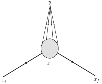
In order to compute the diquark densities in the Random Instanton Liquid Model we start by considering the following Euclidean three-point correlation function:

$$G^{\Gamma}(x_{i},x_{f},y)~{}=~{}\langle 0|~{}J^{\alpha}(x_{f})\,D_{\Gamma}(y)\,\bar{J}^{\alpha}(x_{i})~{}|0\rangle,$$ (59)

where $D_{\Gamma}(y)$ is the diquark density operator defined in (1), and

$$J^{\alpha}(x)=\epsilon^{abc}\,u^{a\,T}(x)\,C\,\gamma_{5}\,d^{b}(x)\,u^{c\,\alpha}(x),\qquad\alpha=1,..,4$$ (60)

is an interpolating operator which excites states with the quantum numbers of the proton. The correlator (59) represents the probability amplitude to create a state with the quantum numbers of a proton at point $x_{i}$, to absorb and re-emit two quarks in a given diquark configuration at a the point $y$, and to finally re-absorb the three-quark state at the point $x_{f}$.

By inserting two complete sets of eigenstates of the QCD Hamiltonian in (59) we obtain:

$$G^{\Gamma}(x_{i},x_{f},y)=\sum_{s,s^{\prime}}\int\frac{d^{3}\,{\bf p^{\prime}}}{2\,\omega_{p^{\prime}}\,(2\pi)^{3}}\int\frac{d^{3}\,{\bf p}}{2\,\omega_{p}\,(2\pi)^{3}}\cdot\,{\textrm{T}r}~{}[\langle 0|\,J(x_{f})\,|\,N({\bf p}^{\prime},s^{\prime})\,\rangle$$

$$\cdot\,\langle N({\bf p}^{\prime},s^{\prime})\,|\,D_{\Gamma}(y)\,|\,N({\bf p},s)\,\rangle\cdot\langle\,N({\bf p},s)|\,\bar{J}(x_{i})\,|\,0\,\rangle]+...,$$ (61)

where $|N({\bf p},s)\rangle$ denotes a proton state of momentum ${\bf p}$ and spin $s$ and the ellipses represent all terms depending on its excitations (including the continuum contribution). In the limit of large Euclidean separations ( $|x_{i}-y|,|x_{i}-x_{f}|$ and $|x_{f}-y|~{}\to~{}\infty$), the contribution from the excited states to the correlation function is exponentially suppressed and only the proton state propagates between the operators.

The overlap of the current operator with the nucleon can be written as:

$$\langle 0|\,J(x_{f})\,|\,N({\bf p}^{\prime},s^{\prime})\,\rangle=~{}\Lambda~{}\mathit{\upsilon}_{s}({\bf p})~{}e^{ip\cdot x_{f}},$$ (62)

where $\mathit{\upsilon}_{s}({\bf p})$ denotes a Dirac spinor. Following stech2 , the matrix elements of the diquark density operator can be parametrized as:

$$\langle N({\bf p^{\prime}},s)|D_{\Gamma}(y)|N({\bf p},s)\rangle=h_{\Gamma}(q^{2})~{}e^{-iq\cdot y}~{}\overline{\mathit{\upsilon}}_{s^{\prime}}({\bf p^{\prime}})~{}\mathit{\upsilon}_{s}({\bf p}).$$ (63)

Substituting (63) and (62) into (III.3) one obtains:

$$G^{\Gamma}(x_{i},x_{f},y) = \Lambda^{2}\,\int\frac{d^{3}\,{\bf p^{\prime}}}{2\,\omega_{p}\,(2\pi)^{3}}\int\frac{d^{3}\,{\bf p}}{2\,\omega_{p^{\prime}}\,(2\pi)^{3}}~{}e^{i(x_{f}\cdot p^{\prime}-x_{i}\cdot p-y\cdot q)}$$ (64)

$$\cdot ~{}h_{\Gamma}(q^{2})~{}\textrm{Tr}~{}\left[(p{\hskip-5.69054pt}/^{\prime}+M)~{}(p{\hskip-5.69054pt}/+M)\right]+...$$

Next, we use the definition of the free fermion propagator in the forward time direction:

$$S(x^{\prime};x)=\int\,\frac{d^{3}{\bf p}}{(2\pi)^{3}\,2\,\omega_{p}}\,e^{i\,p\cdot(x^{\prime}-x)}(p{\hskip-5.69054pt}/+M),\qquad(x^{\prime}_{4}>x_{4})$$

$$=\gamma_{\mu}~{}(x^{\prime}-x)_{\mu}~{}\Pi_{1}(|x^{\prime}-x|)+M~{}\Pi_{2}(|x^{\prime}-x|)$$ (65)

where

$$\Pi_{1}(x) = \frac{-i\,M^{2}}{4\,\pi^{2}~{}x^{2}}~{}\left(K_{0}(M~{}|x|)+\frac{2}{M~{}|x|}~{}K_{1}(M~{}|x|)\right)$$ (66)

$$\Pi_{2}(x) = \frac{i\,M^{2}}{4\,\pi^{2}~{}|x|}~{}K_{1}(M~{}|x|)$$ (67)

and introduce the Fourier transform of the function $h_{\Gamma}(q^{2})$,

$$R_{\Gamma}(z)=\int\frac{d^{4}q}{(2\,\pi)^{4}}~{}e^{i\,z\cdot q}~{}h_{\Gamma}(q^{2}),$$ (68)

We obtain:

$$G^{\Gamma}(x_{i},x_{f},y)=\Lambda^{2}\,\int d^{4}z~{}R_{\Gamma}(y-z)~{}\textrm{Tr}\,[~{}S(x_{f};z)~{}S(z;x_{i})~{}].$$ (69)

The physical interpretation of this result is the following (see also Fig. 1). In the large Euclidean separation limit, the correlator $G^{\Gamma}(x_{i},x_{f},y)$ is governed by the function $R_{\Gamma}(x)$, which encode information about the probability amplitude to find the diquark at a given distance from the center of the nucleon. Notice that $x_{i},x_{f},z$ and $y$ are four-dimensional vectors, so Eq. (69) accounts for relativistic retardation effects. On the other hand, the convolution of $R_{\Gamma}(x)$ with the trace of proton propagators takes into account the center of mass motion.

Figure 1: Graphical representation of the integrand in Eq. (69).

In order to clarify the relationship between the correlator (59) and the diquark density (3) it is instructive to consider first the static approximation for the nucleon, in which $M\to~{}\infty$. In this limit, the proton propagator reads:

$$S(x;y)\simeq\delta({\bf x-y})~{}e^{-M(x_{4}-y_{4})}~{}\frac{(1+\gamma_{4})}{2},$$ (70)

and Eq. (69) becomes:

$$G^{\Gamma}(x_{i},x_{f},y) = 2~{}\Lambda^{2}\,e^{-(x_{f}^{4}-x_{i}^{4})\,M}~{}\delta({\bf x_{f}-x_{i}})~{}\int dz_{4}~{}R_{\Gamma}({\bf r},z_{4}),$$ (71)

where we have used translational invariance to set $y_{4}=0$ and we have introduced ${\bf r}:={\bf y}-{\bf x_{i}}$, the distance between the center of the proton and the position where the diquark is absorbed. The last integral term in this expression represents the time-integrated probability amplitude to find a diquark at a distance ${\bf r}$ from the center of the nucleon. We can therefore identify this quantity with the diquark density (3) defined in section II:

$$\rho_{\Gamma}({\bf r})=~{}\int dz_{4}~{}R_{\Gamma}({\bf r},z_{4}).$$ (72)

Hence, for an infinitely heavy nucleon, the expression relating the correlation function (59) to the diquark density is simply:

$$G^{\Gamma}(x_{i},x_{f},y) = 2~{}\Lambda^{2}\,e^{-(x_{f}^{4}-x_{i}^{4})\,M}~{}\delta({\bf x_{f}-x_{i}})~{}\rho_{\Gamma}({\bf r}).$$ (73)

If the nucleon mass is kept finite, there are corrections to Eq. (73) arising from replacing the static propagator (70) with the exact expression (III.3). As a result, the convolution function $\textrm{Tr}[S(x_{f};z)S(z,x_{i})]$ in (69) $-$ which determines the position of the center of mass of the nucleon $-$ is delocalized on a volume which depends on the Euclidean time $\tau$. We have verified that for a typical mass $M\simeq~{}1$ GeV and a typical Euclidean separation $\tau\simeq$ 1 fm the position of the center of mass of the nucleon is smeared on a volume of radius $\simeq$ 0.3 fm, centered around the origin.

A spatial dependence of the point-to-point propagator is a signal that our nucleon is not at rest. Indeed, in order to isolate completely the zero-momentum component of the nucleon wave-function in our calculation, one would need to use very large Euclidean time separations. However, this would be extremely computationally demanding, because the signal-to-noise ratio for the propagators drop exponentially with the Euclidean time separation.

From these considerations it follows that one should not quantitatively compare the detailed shape of the diquark densities of the Chiral Soliton Model and Constituent Quark Model with that of the Random Instanton Liquid Model. However we shall see below that, as long as one is interested in ratios of diquark densities, it is still possible to draw important qualitative conclusions about the relative strentgh of the diquark correlations.

In this work, we shall estimate ratios of different diquark densities $\rho_{\Gamma^{\prime}}({\bf r})/\rho_{\Gamma}({\bf r})$ by computing ratios of correlation functions $G^{\Gamma^{\prime}}(x_{f},x_{i},y)/G^{\Gamma}(x_{f},x_{i},y)$. Taking ratios allows to maximally reduce the effects of the corrections due to center of mass motion. In fact, such corrections affect in the same way both the numerator and the denominator and do not change the normalization of the correlation function. We have computed (59) choosing ${\bf x}_{i}={\bf x_{f}}=0$, $y=(0,0,r,0)$ and $x^{4}_{f}=-x^{4}_{i}:=\tau$, with $\tau=$ 1 fm. Previous analysis in the Random Instanton Liquid Model have shown that the proton pole is isolated from its excited states for $\tau\gtrsim~{}0.9$ fm baryonRILM ; mymasses ; myformfactors . The numerical calculation has been done averaging over 800 configurations of an ensemble of 492 instantons of $0.33$ fm size, in $V~{}=~{}4.5^{3}~{}\times~{}5.4~{}{\textrm{f}m}^{4}$ box with the topology of a torus. We have used rather large current quark masses ($m_{u}=m_{d}\simeq~{}100MeV$) in order to reduce finite volume artifacts.

Let us comment on the dependence of the Random Instanton Liquid Model predictions on the value of the bare (current) quark mass chosen in our simulations. It is well known that quarks propagating in the instanton vacuum acquire an effective mass associated to the breaking of chiral symmetry. More specifically, the position of the pole of the quark propagator in the instanton background is shifted by an amount $M_{eff}(p,m_{q})$, which depends on both the momentum of the quark $p$ and of its current mass, $m_{q}$.

The dependence of the effective mass on the current quark mass $m_{q}$ has been studied in a number of works, using different approximations (see e.g. mussa and references therein). In all such studies it was found that the sum of the effective mass at zero momentum and the current quark mass $M_{const}=m_{q}+M_{eff}(0,m_{q})$ (which can be interpreted as the constituent quark mass) remains of the order $\simeq~{}350$ MeV for all current masses $m_{q}\lesssim 200$ MeV. In other words, in this model the constituent quark mass is rather insensitive on the the value of the current quark mass. So, we do not expect that the predictions of Random Instanton Liquid Model presented in this work would change dramatically if a smaller current quark mass was used.

III.4 Note on Lattice Calculation of Diquark Densities

We conclude this section by noting that the calculation scheme based on point-to-point correlation functions, used to compute the diquark densities in the Random Instanton Liquid Model, can also be applied to compute the same quantities in Lattice QCD. Conceptually, one needs to replace the average over the configurations of the instanton ensemble with an average over all lattice configurations, performed in the usual way, i.e. by sampling the space of lattice links. Unlike instanton models, lattice QCD calculations are affected by ultraviolet divergences, which are regularized by the lattice spacing. Hence, in a lattice computation, the diquark density operators $D_{\Gamma}({\bf r})$ have to be treated as usual Wilson operators and need to be renormalized.

Figure 2: Predictions for the ratio $R_{1}(r)=\rho_{\gamma_{3}}({\bf r})/\rho_{\gamma_{5}}({\bf r})$ in the Non-Relativistic Quark Model (NRQM), in the Random Instanton Liquid Model (RILM) and in the Chiral Soliton Model (CSM). The CSM results include the projection onto the proton state.

IV Comparison and Discussion

In this session, we discuss the results of the phenomenological calculations presented in the previous session. We choose to consider only the ratios constructed by dividing the densities $\rho_{\gamma_{3}}({\bf r})$. $\rho_{\gamma_{4}\,\gamma_{5}}({\bf r})$ and $\rho_{\gamma_{4}}({\bf r})$ by the scalar density $\rho_{\gamma_{5}}({\bf r})$. There are several reasons for this choice. In general, ratios are less model dependent than the individual densities. For example, in the Non-Relativistic Quark Model, they are completely insensitive to the details of the spatial wave function. Moreover, in lattice and Random Instanton Liquid Model calculations, taking ratios allow to remove the dependence on the Proton Mass, Euclidean time and the coupling $\Lambda$ (see Eq. (73)). We shall not discuss the ratio constructed with the $\rho_{1}({\bf r})$ density, as it is identically zero in all the models we have considered.

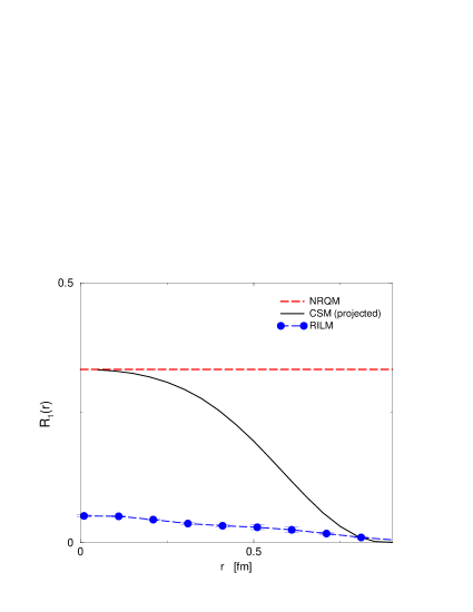
Let us first analyze the ratio constructed with the density of axial-vector and scalar diquarks:

$$R_{1}({\bf r})=\frac{\rho_{\gamma_{3}}({\bf r})}{\rho_{\gamma_{5}}({\bf r})}.$$ (74)

The results of our phenomenological calculations are shown in Fig. 2. In the $SU(6)$ Non-Relativistic Quark Model, this ratio is completely determined by the $SU(6)$ spin-flavor structure of the wave-function, and is identically equal to 1/3. In the Random Instanton Liquid Model, $R_{1}({\bf r})$ is sizebly reduced in magnitude (by a factor $\simeq~{}5$). In the Chiral Soliton Model, at ${\bf r}=0$ the $p$-wave contribution from the lower components of the spinors vanishes and one recovers the Non-Relativistic Quark Model Results. On the other hand, the axial-vector diquark density drops down very rapidly at the border of the soliton, where the pion field is most intense.

These results can be interpreted as follows. In the Random Instanton Liquid Model, the spin- and flavor- dependent ’t Hooft interaction generates a strong attraction which enhances the probability amplitude of finding two quarks in the same point in the $0^{+}$ anti-triplet configuration, relative to the amplitude of finding them in the $1^{+}$ configuration. This explains why the Random Instanton Liquid Model prediction for $R_{1}({\bf r})$ is much smaller than that of the $SU(6)$ Non-Relativistic Quark Model and the Chiral Soliton Model. The discrepancy between Random Instanton Liquid Model and mean-field Chiral Soliton Model calculations is a signal that in the instanton vacuum at $N_{c}=3$ there are strong two-body correlations, which are not captured by the large $N_{c}$ approximation.

From this comparison it follows that a lattice calculation of $R_{1}({\bf r})$ could provide information about the strength of scalar diquark correlations in the nucleon. If the non-perturbative QCD interactions generate a strong correlation in the $0^{+}$ anti-triplet channel, as assumed in the Jaffe-Wilczek model, then we predict that the curve obtained from a lattice calculation should lie much below 1/3. If lattice simulations found that $R_{1}({\bf r})\sim 1/3$, then this would imply that diquarks are not particularly correlated in the $0^{+}$ diquark channel and therefore the Jaffe-Wilczek picture is not correct. $R_{1}({\bf r})>1/3$ would represent an indication that the quark-quark interaction is less attractive in the $0^{+}$ channel, relative to the $1^{+}$ channel. This would certainly be a very surprising result, since the ($\bar{{\bf 3}}_{c},~{}\bar{{\bf 3}}_{f}$) channel is favored by both the perturbative and the instanton-mediated interactions.

Unfortunately, the ratio $R_{1}({\bf r})$ does not encode information about the microscopic dynamical mechanism underlying such diquark correlations. In fact, two completely different quark-quark effective interactions (e.g. one with a chirality-conserving vertex and one with a chirality-flipping vertex) may lead to the same predictions, as long as the short-range attraction in the scalar channel is sufficiently strong.

In order to gain some insight on the microscopic origin of diquarks we need to analyze a different ratio:

$$R_{2}({\bf r})=\frac{\rho_{\gamma_{5}\,\gamma_{4}}({\bf r})}{\rho_{\gamma_{5}}({\bf r})}.$$ (75)

The results of our calculations in the three phenomenological models are reported in Fig. 3. In the Non-Relativistic Quark Model, both the $\rho_{\gamma_{5}}({\bf r})$ and $\rho_{\gamma_{5}\,\gamma_{4}}({\bf r})$ densities probe the $0^{+}$ scalar diquark content of the proton, so $R_{2}({\bf r})=1$. In the Random Instanton Liquid Model the magnitude of this ratio is smaller than in the Non-Relativistic Quark Model, by a factor 3 or so. The fact that, in the Random Instanton Liquid Model, $R_{2}({\bf r})\ll 1$ has an important dynamical explanation. It is due to the different sensitivity of the numerator and denominator to the so-called direct-instanton contribution. The $\rho_{\gamma_{5}}({\bf r})$ diquark density receives maximal contribution from the interaction of quarks with the field of the closest (direct) instanton, in the vacuum. This statement can be verified by computing the correlator in the single-instanton approximation, discussed in SIA . On the other hand, the density in the numerator, $\rho_{\gamma_{5}\,\gamma_{4}}({\bf r})$ does not receive such a direct-instanton contribution and instanton-induced effects come only from the interactions of quarks with many instantons. The magnitude of the latter contributions are parametrically suppressed by the diluteness of the instanton vacuum, $\kappa=\bar{n}\,\bar{\rho}^{4}\ll~{}1$. Physically, this is the same reason why vector and axial-vector channels have a rather large “Zweig rule”, forbidding flavor mixing, while for scalar and pseudo-scalar channels such a mixing is very strong.

We remark that the very strong channel dependence of hadronic correlation functions is a well-known dynamical implication of instanton models. It is quite hard to obtain this effect in alternative dynamical mechanisms (for a detailed discussion see shuryakcorr ). This was initially pointed out by Novikov, Shifman, Vainstein and Zakharov, in the context of Operator Product Expansion (OPE) and QCD sum-rules for hadronic correlation functions areallhadronsalike . Diquark correlations induced by the direct instantons were discussed also in kochelev1 .

In the Chiral Soliton Model, the ratio $R_{2}({\bf r})$ remains of order 1 for $|{\bf r}|\lesssim~{}1$ fm and drops rapidly at the border of the soliton. The significant deviation of the Chiral Soliton Model result from the Random Instanton Liquid Model prediction shows that a mean-field approach does not capture correlations associated to the direct-instanton effects.

Figure 3: Predictions for the ratio $R_{2}({\bf r})=\rho_{\gamma_{4}\gamma_{5}}({\bf r})/\rho_{\gamma_{5}}({\bf r})$, in the Non-Relativistic Quark Model (NRQM), in the Random Instanton Liquid Model (RILM) and in the Chiral Soliton Model (CSM).

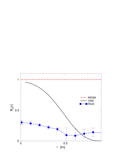
From this discussion it follows that, if the scalar diquark correlations are mainly induced by instantons or in general by a Nambu-Jona-Lasinio type of interaction (i.e. chirally symmetric, with a chirality flipping vertex), then a lattice measurement should give $\rho_{\gamma_{4}\gamma_{5}}({\bf r})\ll\rho_{\gamma_{5}}({\bf r})$, so $R_{2}({\bf r})\ll~{}1$.

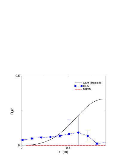
Let us now analyze a third ratio:

$$R_{3}({\bf r})=\frac{\rho_{\gamma_{4}}({\bf r})}{\rho_{\gamma_{5}}({\bf r})}.$$ (76)

The results of our calculations in the three phenomenological models are reported in Fig. 4. This quantity is identically zero in the Non-Relativistic Quark Model, so it represents a probe of relativistic effects in the nucleon. The ratio is also rather small in the Random Instanton Liquid Model, denoting that quarks propagating in the nucleon receive small relativistic corrections. On the contrary, $R_{3}({\bf r})$ in the Chiral Soliton Model increases rapidly and approaches 1/3, near the border of the soliton. The interpretation of this result is the following. Near the edge of the soliton, the quark field changes very rapidly. This rapid change gives rise to a large derivative of the wave-function in coordinate space or, equivalently, to large high-p components, in momentum space. Such modes enhance the contribution from the lower components of the spinor wave-function, which give rise to relativistic corrections.

Figure 4: Predictions for the ratio $R_{3}({\bf r})=\rho_{\gamma_{4}}({\bf r})/\rho_{\gamma_{5}}({\bf r})$ in the Non-Relativistic Quark Model (NRQM), in the Random Instanton Liquid Model (RILM) and in the Chiral Soliton Model (CSM). The CSM results include the projection onto the proton state. The Non-Relativistic Quark Model curve is identically zero.

V Physical Properties of the Scalar Diquark in the Instanton Vacuum

In the previous section we have shown that instantons generate a strong attraction between a $u$ and a $d$ quark in the color anti-triplet $0^{+}$ channel. In this section, we provide unambiguous evidence that such forces are strong enough to form a bound diquark state. We also estimate the diquark size by computing its electric charge radius in the Random Instanton Liquid Model.

V.1 Mass of the scalar diquark

The question if instanton models lead to a bound $0^{+}$ color anti-triplet diquark has been first posed by Diakonov and Petrov petrov and investigated in a number of works. In an exploratory study baryonRILM Shuryak, Schäfer and Verbaarshot computed some diquark two-point functions in coordinate space, using the Random Instanton Liquid Model. They found some evidence for a light diquark bound-state (of rougly 450 MeV mass), by performing an analysis of the correlation function, based on a pole-plus-continuum parametrization of the spectral density. On the other hand, Diakonov, Petrov and collaborators have analyzed diquarks by solving Schwinger-Dyson equations at the leading order in $1/N_{c}$ diak . They found evidence for correlations, but no binding.

In order to clarify this issue, we have followed an approach which is usually applied to extract hadron masses in lattice simulations. As usual, we have replaced the average over all gauge configurations with an average over the configurations of the instanton ensemble. This method presents some advantages with respect to the coordinate-representation calculation of Shuryak et al. On the one hand, it avoids the undesired additional model dependence associated with the parametrization of the spectral function. On the other hand, it makes unambiguously evident the existence of the bound state and allows to determine more precisely its mass.

The starting point consists of computing the Euclidean two-point function:

$$G2(\tau)=\int d^{3}{\bf r}~{}\langle 0|~{}T[~{}J_{D}({\bf 0},\tau)J^{\dagger}_{D}({\bf r},0)\,Pe^{\int dy_{\mu}A_{\mu}(y)}~{}]|0\rangle,$$ (77)

where $J_{D}(x)$ is the usual diquark current:

$$J^{a}_{D}(x)=\epsilon^{abc}\,u^{b\,T}(x)\,C\,\gamma_{5}\,d^{c}(x).$$ (78)

The path-ordered exponent in (77) represents a Wilson line connecting the two extremes of the two-point function and is needed to assure gauge invariance of the correlator. In the instanton vacuum, the contribution from the Wilson line is very small, as heavy quarks couple very weakly with instantons.

In the large Euclidean time limit, only the lightest state with the quantum numbers of the current $J_{D}(x)$ propagates in the two-point function. If there is a diquark bound-state, then, in the large Euclidean time limit, the logarithm of the two-point function must scale linearly with $\tau$:

$$\ln G2(\tau)\stackrel{{\scriptstyle\tau\to\infty}}{{\rightarrow}}\ln\Lambda_{D}^{2}-\tau~{}M_{D},$$ (79)

where $M_{D}$ is the mass of the diquark and the constant $\Lambda_{D}$ is its coupling to the current, defined by $\langle 0|J_{D}(0)|D\rangle=~{}\Lambda_{D}$.

We have computed such a correlation function in the Random Instanton Liquid Model, averaging over 100 configurations in a $4^{3}~{}\times~{}8~{}\textrm{fm}^{4}$ box. In analogy with lattice simulations, a rather large quark mass was needed to reduce the finite-volume artifacts. The result for our calculation of the correlation function (77) with $m_{q}\simeq~{}100$ MeV is shown in Fig. 5.

Figure 5: Logarithm of the diquark two-point function, $\ln G2(\tau)$ computed in the Random Instanton Liquid Model. The linear slope is a clean signature of the existence of a bound state.

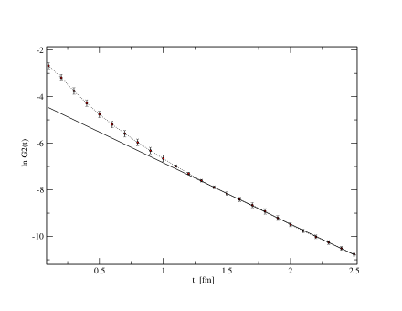
We clearly see that, in the large $\tau$ limit, the logarithm of the two-point function becomes a linear function of $\tau$.

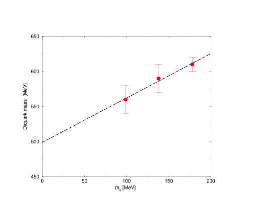
In order to study the sensitivity of the diquark mass on the current quark mass, we have computed the correlation function for different values of the $u$ and $d$ quark mass, $m_{u}=m_{d}=m_{q}=\{180,~{}140,~{}100\}~{}$MeV. The dependence of diquarks mass on the current quark masses is plotted in Fig. 6. A rough estimate of the diquark mass can be obtained by linearly extrapolating to the physical value of the current quark mass. We find a diquark mass of $\sim~{}500$ MeV, in good agreement with the previous estimate.

V.2 Diquark size

An important question to address is the size of the diquark. From general arguments, we expect that it should be comparable with the size of the proton. In fact even the most tightly bound QCD excitation, the pion, is known to have a rather large electric charge square radius, $r_{E}^{\pi}\simeq~{}0.6$ fm. On the other hand, an early naive analysis in the Instanton Liquid Model 3ptILM gave a surprisingly small estimate for the diquark charge radius, $r_{E}\sim~{}0.3$ fm. It is hard to estimate the accuracy of such an estimate which was based on a number of assumptions. Hence, it is worth performing a direct calculation of the diquark electro-magnetic form factor.

To this end, we have computed the diquark electro-magnetic three-point function,

$$G3_{D}(\tau,{\bf q})=\int d^{3}{\bf y}\,d^{3}{\bf x}~{}e^{i~{}{\bf q}\cdot{\bf y}}~{}\langle 0|~{}T[~{}J_{D}({\bf 0},\tau)~{}J^{e/m}_{4}({\bf y},0)~{}J^{\dagger}_{D}({\bf x},-\tau)~{}Pe^{\int dy_{\mu}A_{\mu}(y)}~{}]|0\rangle$$ (80)

where $J_{D}(x)$ is the usual diquark interpolating operator and $J^{e/m}_{\mu}(x)=2/3~{}\overline{u}(x)~{}\gamma_{\mu}~{}u(x)-1/3~{}\overline{d}(x)~{}\gamma_{\mu}~{}d(x)$ is the electro-magnetic current operator. In the large $\tau$ limit, the correlation functions (80) relates directly to the diquark form factor , $F_{D}(Q^{2})$:

$$G3_{D}(\tau,{\bf q})\stackrel{{\scriptstyle\tau\to\infty}}{{\rightarrow}}\Lambda_{D}^{2}~{}e^{-(M+\sqrt{M_{D}^{2}+{\bf q}^{2}})\tau}~{}F_{D}(Q^{2}),$$ (81)

where the values of the diquark mass and the constant $\Lambda_{D}$ can be extracted from the two-point correlation function.

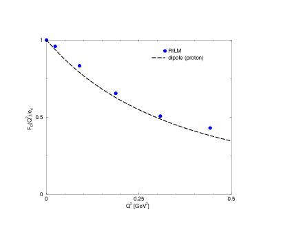
The result of the Random Instanton Liquid Model calculation of the form factor (normalized to the total $u-d$ diquark charge, $e_{D}=1/3$ ) is presented in Fig. 7, where it is compared to the phenomenological dipole fit which reproduces the low-energy data on the proton electric form factor. These results imply that the diquark is an extended object, whose size is comparable with that of the nucleon. Its electric charge radius is found to be $r_{E}^{2}\textrm{(diquark)}\simeq(0.70~{}\textrm{fm})^{2}$, which should be compared to the value of the electric charge radius of the proton, $r_{E}^{2}\textrm{(proton)}\simeq(0.76~{}\textrm{fm})^{2}$ computed in the Random Instanton Liquid Model in myformfactors . As expected, the electric charge radius of the diquark is larger than that of the pion and smaller than that of the proton.

VI Conclusions

Figure 6: The mass of the u-d diquark, computed in the Random Instanton Liquid Model, as a function of the $u$ and $d$ bare quark mass.

In this work we have addressed the question of how is it possible to study two-body diquark correlations in hadrons, using lattice QCD. We have identified some suitable lattice-calculable correlation functions, which allow to probe directly the diquark content of the nucleon. We have argued that these Green’s functions provide important information about non-perturbative correlations, in different color anti-triplet diquark channels.

In particular, the ratio $R_{1}({\bf r})$, defined in Eq. (74), measures the strength of the correlations in the scalar diquark channel, relative to that in the axial-vector channel. It can be used to check the main dynamical assumption of the Jaffe-Wilczek model. In fact, if the quark-diquark picture is correct, then we predict that a lattice measurement must lead to $R_{1}({\bf r})\ll 1/3$.

The ratio $R_{2}({\bf r})$, defined in Eq. (75), can be used to gain some insight on the dynamical origin of the non-perturbative interaction in the scalar diquark channel. In particular, it can be used to check the hypothesis according to which these forces are mediated by instantons (or more generally by a NJL-like, chirality-flipping interaction). We have argued that, in this case, we expect that lattice measurements should give $R_{2}({\bf r})\ll 1$.

We have computed these ratios using three phenomenological models. We have found that they lead to radically different predictions for the matrix elements we have selected. Hence, a lattice measurement could point out which picture is most realistic. It is worth stressing that from the fact that the Chiral Soliton Model predictions differ substantially from the Random Instanton Liquid Model results one should not conclude that the Chiral Soliton Model is not correctly reproducing the physics of instanton-induced interactions. In fact, such mean-field model can account for one-body local operators. On the other hand, our results show that it is much less reliable for computing matrix elements of two-body operators. The discrepancy between Random Instanton Liquid Model and Chiral Soliton Model should be taken as an indication that rather strong direct two-body correlations are generated in the instanton vacuum.

We would like to stress that the qualitative differences between the predictions of the three models considered in the present analysis are dramatic and therefore quite robust. However, one should be careful in comparing the details of the curves associated to the diquark density ratios, at a quantitative level. In fact, on the one hand, the Random Instanton Liquid Model predictions are affected by the smearing effects associated to the center of mass motion (see the discussion in section III.3). On the other hand, the Chiral Soliton Model and the Random Instanton Liquid Model calculations are performed using different values  of the current quark mass $m_{q}$. This fact may reflect itself in a slightly different value of the effective mass of the quarks propagating in the chirally broken vacuum (see the discussion at the end of section III.3).

In the second part of the work, we have studied in detail the physical properties of instanton-induced diquarks. We have provided unambiguous evidence that instantons generate a scalar diquark bound-state of mass $\sim~{}500$ MeV, in good agreement with earlier estimates based on point-to-point correlation functions in coordinate space.

We have also studied its electric charge distribution. Our results show that the scalar diquark is an extended object, whose size is of the order of the fm, hence comparable with that of the proton. Thus, phenomenological quark-diquark models cannot treat the diquark as a point-like object.

As a concluding remark, we stress that the analysis performed in this work focused on the diquark content of the proton. However, the same study could be repeated, in order to investigate the diquark content of other lowest-lying baryons. For example, it would be particularly interesting to compare the diquark densities in the nucleon and in the delta. In fact, in the delta, the leading direct-instanton effects are suppressed, due to the Dirac- and flavor- structure of the ’t Hooft interaction. Hence, if diquark correlations are instanton-mediated, then we expect that the strong enhancement of the scalar density observed in the proton should be much less pronounced in the delta.

Figure 7: The diquark form factor (normalized to the total charge) evaluated in the Random Instanton Liquid Model (points) and compared with the dipole parametrization of the low-energy data on proton electric form factor: $F_{dip}=1/(1+Q^{2}/0.71)^{2}$ (dashed line). The numerical simulation was performed in a $(4^{3}\times 6)~{}\textrm{fm}^{4}$ box and the exchanged momentum is quantized accordingly.