hep-ph/0410302

Hierarchical Quark Masses and Small Mixing Angles
from Warped Intersecting Brane Models

Tatsuya Noguchi

^∗Tohoku University, Miyagi 980-8578, Japan

We propose a novel mechanism for reproducing the realistic hierarchical structure of the observed CKM mixing matrix and quark masses by means of introducing a warped metric. We illustrate the method on the basis of a specific Type IIA intersecting brane model proposed by Ibáñez et al. The model is compactified on a direct product of three tori, on which four D-brane stacks wrap, and the intersections between two stacks collectively provide three generations of quarks and leptons. The exponential of the area formed by the intersection points corresponding to three matter fields is interpreted as the Yukawa coupling among them. It is known, however, that the Yukawa matrices for quarks are generically singular, and that it does not give definite mixing angles nor hierarchically suppressed quark masses. We show that the newly introduced warp effect on the internal manifold modifies the Yukawa matrix elements and generate hierarchical quark masses and CKM mixing angles.

1 Introduction

The string theories have been regarded as one of the most promising models for describing both gravity and particle physics. Many researchers have tried to derive the Standard Model within the framework. Since the theories are originally constructed in higher dimensional spacetime, the extra dimensions must be compactified on some manifold. Through these procedure, in most cases, there appear many scalar fields at low energy scale, and their vacuum expectation values remain unfixed because we cannot calculate the potentials of these fields within the perturbative framework.

In the mid-1990s, the author in Ref. [1] formulated D-branes, spatially extended objects, on the worldsheet of string theories by imposing Dirichlet boundary conditions on the end points of strings. It is found that D-branes carry a certain amount of Ramond-Ramond charge, and that they could be regarded as solitons in supergravity theories. The emergence of solitons, as is known from quantum field theories, suggests a duality transformation from one theory described in terms of a certain set of fundamental fields and couplings to another in different terms. This string duality shed light on the relation among string theories, and invoked a considerable number of studies on the construction of phenomenological models with D-branes in Type IIA, Type IIB, and Type I string theories although they are once regarded inadequate for explaining the real world.

Recently, intersecting D-brane models have been intensively studied. The scenario was first proposed by Blumenhagen et al. in the context of Type I string theory [2, 3, 4]. On a stack of $N$ D-branes, the charges assigned to the end points of open strings, called Chan-Paton factors, are known to form collectively the adjoint representation of $U(N)$ gauge group. Furthermore, at the intersection between a stack of $N$ D-branes and that of $M$ D-branes there appears a massless fermionic field belonging to a bifundamental representation $(N,\bar{M})$ of a gauge group $U(N)\times U(M)$ [5, 6]. In the framework of intersecting brane models, these massless open string modes are identified with matter fields such as quarks and leptons. It is worth noting that a Yukawa coupling is described as $e^{-kA}$, where $k$ is a constant of order 1, and $A$ is the area formed by three intersecting points corresponding to the relevant matter fields. Since the superstring theories are constructed in 10 dimensional spacetime, we have to compactify them on 6 dimensional manifold when it comes to discussing phenomenology. In that case, D-branes wrap on some cycles of the manifold and they generically intersect with each other several times, and the intersection numbers determine the number of matter fields. Many researchers have investigated intersecting brane models in various aspects: the search for the standard model [7, 8, 9, 10, 11] , the construction of grand unified theories[12, 13, 14, 15], supersymmetric models [16, 17, 18, 19] and composite models[20, 21], the CFT calculation of couplings between fields locating at intersections[23, 24, 25], quark masses and a CKM mixing matrix [11, 21, 22, 26], and phenomenological viability[27, 28, 29].

In this paper, we focus on a specific Type IIA intersecting brane model compactified on a direct product of three tori proposed by Ibáñez et al.[9] In the model, the family of right-handed quarks is distinguished by the difference of intersecting points in position on the first torus, and that of left-handed ones on the third torus. The Yukawa matrices are described by the area formed by three intersecting points corresponding to quarks and a Higgs boson. Owing to the direct product structure of the internal manifold, the Yukawa matrices take the form of $a_{i}b_{j}^{U/D}$ and have only one non-zero eigenvalue, which is identified to be the third generation quark mass. In addition, we cannot obtain a definite CKM mixing matrix in the model. In this paper, we investigate quark masses and a CKM mixing matrix assuming a warp effect on the internal manifold, i.e., the dependence of the first torus volume on a coordinate of the third one. We reproduce the realistic hierarchical structure of the observed CKM mixing matrix and quark masses under some condition on small parameters originated from the warp effect and the size of tori.

The outline of our paper is as follows. In section 2, we briefly review the construction of intersecting brane models. In section 3, assuming a warp effect on tori we calculate the Yukawa matrices and obtain the mass spectra for quarks and the CKM matrix. We show that our model reproduces the realistic hierarchical structure with several small parameters determined properly. The section 4 is devoted to the discussion.

2 Intersecting Brane Models

We briefly review an intersecting brane model presented in Ref.  [9]. We consider Type IIA string theory compactified on orientifold six tori, with several stacks of D-branes intersecting each other at angles. Let us assume that orientifolds are located at $x_{4}=0,\pi$, $x_{6}=0,\pi$ and $x_{8}=0,\pi$, and that D6-branes wrapped on a direct product of 1-cycles of each torus $T^{i}$ with a set of winding numbers $(n_{a}^{i},m_{a}^{i})$. The intersection is four dimensional. We know that at the intersection between $N_{a}$ D6-branes and $N_{b}$ D6-branes, there is an $(N_{a},\bar{N}_{b})$ representation of the gauge group $U(N_{a})\times U(N_{b})$. In our setup, there are also mirror branes owing to the orientifolds. The winding number of mirror branes are described as $(n_{a}^{i},-m_{a}^{i})$. Later on, two sectors play an important role in generating quarks and leptons. The first sector $D_{a}$-$D_{b}$, realized on the intersection between two D-brane stacks, D$6_{a}$-branes and D$6_{b}$-branes. The intersection number turns out to be

$$I_{ab} = (n_{a}^{1}m_{b}^{1}-n_{b}^{1}m_{a}^{1})(n_{a}^{2}m_{b}^{2}-n_{b}^{2}m_{a}^{2})(n_{a}^{3}m_{b}^{3}-n_{b}^{3}m_{a}^{3}),$$ (2.1)

and the sector gives a bifundamental representation $(N_{a},\bar{N}_{b})$. The second sector $D_{a}$-$\Omega D_{b}$ is realized on the intersection between $D6_{a}$-branes and a mirror stack corresponding to another D-brane stack, $\bar{D}6_{b}$-branes. The intersection number is

$$I_{ab} = -(n_{a}^{1}m_{b}^{1}+n_{b}^{1}m_{a}^{1})(n_{a}^{2}m_{b}^{2}+n_{b}^{2}m_{a}^{2})(n_{a}^{3}m_{b}^{3}+n_{b}^{3}m_{a}^{3}),$$ (2.2)

and it gives a representation $(N_{a},N_{b})$. A negative sign in (2.1) and (2.2) represents the opposite chirality. The other sectors are not relevant to our discussion.

So far, we have not imposed any restriction on winding numbers. We have to take account of Ramond-Ramond tadpole cancellation condition, which means the cancellation of D-brane charge on the internal manifold. If there is no orientifold, the condition is described as

$$\prod_{a}^{K}N_{a}\Pi_{a}=0,$$ (2.3)

i.e. the sum of the cycles on which D-branes wrap is equal to zero. If there are several orientifolds, they play a role of negatively charged objects. In our setup, the orientifold planes wrapping on a cycle $(1,0),(1,0),(1,0)$, the condition reads

$$\sum_{a}N_{a}n_{a}^{1}n_{a}^{2}n_{a}^{3} = 16,$$

$$\sum_{a}N_{a}m_{a}^{1}m_{a}^{2}n_{a}^{3} = 0,$$

$$\sum_{a}N_{a}m_{a}^{1}n_{a}^{2}m_{a}^{3} = 0,$$

$$\sum_{a}N_{a}n_{a}^{1}m_{a}^{2}m_{a}^{3} = 0.$$ (2.4)

We should consider the possibility of NS B-flux $b^{i}$ on a torus $T^{i}$ [4]. Starting with Type I string theory compactified on a direct product of three tori, the introduction of NS B-flux background $b=1/2$ on a torus modifies its complex structure. In the intersecting brane picture, the effect is equivalent to changing a winding number on an original torus $(n,m^{\prime})$ into $(n,m^{\prime}+n/2)$. We will describe the configuration of D-branes in terms of this newly defined effective winding number $m=m^{\prime}+n/2$ on a torus with non-zero $B$-field background.

We are now ready to look for winding numbers generating standard model matter fields:

$Q_{L}^{i}=(3,2,1/6);\quad U_{R}^{i}=(\bar{3},1,-2/3);\quad D_{R}^{i}=(\bar{3},1,1/3);$

$L^{i}=(1,2,-1/2);\quad E_{R}^{i}=(1,1,1)$.

Note that we have to put at least four stacks of D-branes. This is because the right-handed charged lepton $E_{R}^{i}$ does not have the charge of $SU(3)$ nor that of $SU(2)$, thus at least two more D-brane stacks are required. From now on, we discuss the models with four D-brane stacks: stack $a$ composed of 3 D6-branes, stack $b$ of 2 D6-branes, and the others composed of a D6-brane.

First, the requirement of the above matter fields allows only the winding numbers denoted in Table 1, where $\beta^{i}=1-b^{i}$, $\epsilon=\pm 1$ and $\rho=1,1/3$. The variables $n_{a}^{2}$, $n_{b}^{1}$, $n_{c}^{1}$ and $n_{d}^{2}$ take integers. Note that on the third torus, the $B$ field always takes a value $b^{3}=1/2$. This model contains four $U(1)$ charges originated from D-brane stacks $Q_{a}$, $Q_{b}$, $Q_{c}$, and $Q_{d}$. Each of them can be understood in terms of the Standard Model framework:

$$Q_{a}=3B,\quad Q_{c}=2I_{R},\quad Q_{d}=-L,$$ (2.5)

where $B$ is the baryon number, $L$ is the lepton number, and $I_{R}$ is the third component of right-handed weak isospins. $Q_{b}$ plays a role of a generation dependent Peccei-Quinn symmetry. Owing to the couplings to the Ramond-Ramond fields, three of the four $U(1)$ charges become massive and only the gauge boson corresponding to the hypercharge

$$Q_{Y}=\frac{1}{6}Q_{a}-\frac{1}{2}Q_{c}+\frac{1}{2}Q_{d}$$ (2.6)

remains massless if and only if the following relation holds:

$$n_{c}^{1} = \frac{\beta^{2}}{2\beta^{1}}(n_{a}^{2}+3\rho n_{d}^{2}).$$ (2.7)

$N_{i}$	$(n_{i}^{1},m_{i}^{1})$	$(n_{i}^{2},m_{i}^{2})$	$(n_{i}^{3},m_{i}^{3})$
$N_{a}=3$	$(1/\beta^{1},0)$	$(n_{a}^{2},\epsilon\beta^{2})$	$(1/\rho,1/2)$
$N_{b}=2$	$(n_{b}^{1},-\epsilon\beta^{1})$	$(1/\beta^{2},0)$	$(1,3\rho/2)$
$N_{c}=1$	$(n_{c}^{1},3\rho\epsilon\beta^{1})$	$(1/\beta^{2},0)$	$(0,1)$
$N_{d}=1$	$(1/\beta^{1},0)$	$(n_{d}^{2},-\beta^{2}\epsilon/\rho)$	$(1,3\rho/2)$

Table 1: The winding numbers yielding the Standard Model matter fields.

Secondly, as for the tadpole cancellation, these winding numbers satisfy automatically all but the first condition of Eqs. (2). It reads

$$\frac{3n_{a}^{2}}{\rho\beta^{1}}+\frac{2n_{b}^{1}}{\beta^{2}}+\frac{n_{d}^{2}}{\beta^{1}}=16.$$ (2.8)

If there are more than four D-brane stacks, their contribution should be added to the left handed side of Eq. (2.8). It is possible to satisfy tadpole cancellation conditions by adding some D-brane stacks which do not intersect with the first four stacks, i.e. keeping the intersection numbers the same.

In conclusion, the desired configuration is realized by the winding numbers defined in Table 1 with the parameters satisfying Eqs. (2.7) and (2.8). The resultant matter contents and their $U(1)$ charges are shown in Table 3. We are now ready to consider the Yukawa couplings. For simplicity, we take a specific D-brane configuration and calculate the Yukawa matrices

$$\beta^{1}=\beta^{2}=1,\qquad\quad\;$$ (2.9)

$$\epsilon=-1,\quad\rho=1,\qquad\quad$$ (2.10)

$$a^{2}=2,\;n_{b}^{1}=0,\;n_{c}^{1}=1,\;n_{d}^{2}=0.$$ (2.11)

$N_{i}$	$(n_{i}^{1},m_{i}^{1})$	$(n_{i}^{2},m_{i}^{2})$	$(n_{i}^{3},m_{i}^{3})$
$N_{a}=3$	$(1,0)$	$(2,-1)$	$(1,1/2)$
$N_{b}=2$	$(0,1)$	$(1,0)$	$(1,3/2)$
$N_{c}=1$	$(1,-3)$	$(1,0)$	$(0,1)$
$N_{d}=1$	$(1,0)$	$(0,1)$	$(1,3/2)$

Table 2: A combination of winding numbers yielding the SM matter fields

Intersection	Matter fields	repr.	$Q_{a}$	$Q_{b}$	$Q_{c}$	$Q_{d}$	$Y$
$(a,b)$	$Q_{L}$	$(3,2)$	$1$	$-1$	$0$	$0$	$1/6$
$(a,b^{*})$	$q_{L}$	$2(3,2)$	$1$	$1$	$0$	$0$	$1/6$
$(a,c)$	$U_{R}$	$3(\bar{3},1)$	$-1$	$0$	$1$	$0$	$-2/3$
$(a,c^{*})$	$D_{R}$	3$(\bar{3},1)$	$-1$	$0$	$-1$	$0$	$1/3$
$(b,d^{*})$	$L$	$3(1,2)$	$0$	$-1$	$0$	$-1$	$-1/2$
$(c,d)$	$E_{R}$	$3(1,1)$	$0$	$0$	$-1$	$1$	$1$
$(c,d^{*})$	$N_{R}$	$3(1,1)$	$0$	$0$	$1$	$1$	$0$

Table 3: Matter contents and $U(1)$ charges

The brane configuration of this setup is depicted in Fig. 1, where we take specific values for moduli parameters indicating positions of branes. In order to satisfy the first tadpole cancellation condition, we add 5 parallel D-branes with a winding number $(1,0)\;(1,0)\;(1,0)$, which do not intersect with any D-brane stacks.

In this context, the Higgs scalar fields come from the open string modes stretching from two parallel D-brane stacks not from an intersection. These modes are tachyonic, and are expected to undergo tachyon condensation, which could be liken to the Higgs mechanism, and to become finally ordinary Higgs fields with appropriate masses. Nevertheless, the mechanism of condensation has not been clarified. For the purpose of avoiding the complexity on the tachyon condensation, we assume that the size of the second torus is so small compared with the others that we neglect it when evaluating Yukawa couplings.

This model has the following Yukawa interactions:

$$y_{j}^{U}Q_{L}U_{R}^{j}h_{1}+y_{j}^{D}Q_{L}D_{R}^{j}H_{2}$$ (2.12)

$$+ y_{ij}^{u}q_{L}^{i}U_{R}^{j}H_{1}+y_{ij}^{d}q_{L}^{i}D_{R}^{j}h_{2}$$

$$+ y_{ij}^{L}L^{i}E_{R}^{j}H_{2}+y_{ij}^{N}L^{i}N_{R}^{j}h_{1}+\mbox{h.c.}$$

where $Q_{L}$ and $q_{L}^{i}(i=1,2)$ are left-handed quarks, $U_{R}^{j}(j=1,2,3)$ are right-handed ones, and $h_{1}$, $h_{2}$, $H_{1}$, and $H_{2}$ are Higgs fields. The coefficients $y^{U},y^{D},y^{u},y^{d},y^{L}$, and $y^{N}$ are Yukawa couplings. Each of them is described by the triangular area $A_{ijk}$ formed by three intersecting points corresponding to the fields included in the Yukawa interaction term

$$y_{ijk}=e^{-kA_{ijk}},$$ (2.13)

where $k$ is a constant of order 1, which is expected to be fixed through stringy calculation[23, 24].

This expression can be interpreted intuitively as follows. All the matter fields such as quarks and leptons come from open string modes, with one end on a stack and the other end on the other stack. For example, $Q_{L}^{1}$ has one end on D$6_{a}$-branes and the other on D$6_{b}$-branes. Likewise, $U_{R}^{1}$ is the open string mode stretching between D$6_{b}$-branes and D$6_{c}$-branes, and $h_{1}$ between D$6_{c}$-branes and D$6_{a}$-branes. The Yukawa coupling among these three fields evaluated by the scattering amplitude among these open strings, i.e., by the exponential of the area swept by them. When the compact manifold is a direct product of tori, Yukawa couplings are expressed by the sum of the triangular areas projected on each torus $A_{ijk}^{(n)}$[11]:

$$A_{ijk}=\sum_{n=1}^{3}A_{ijk}^{(n)}.$$ (2.14)

Before we come to the main subject, we must draw attention to the stability of intersecting brane models. It is known that, in general, parallel D-branes do not attract each other because of the cancellation between the repulsive force coming from RR sectors and the attractive one from NS sectors. However, as for D-branes intersecting at angles, this is not the case. Besides the massless fermion states, in general, there are some scalar states at each intersection, which could be regarded as supersymmetric partners of the fermion states. The mass square of these scalar states is parameterized by the angles between two D-brane stacks. Some choices of angles give a negative mass square, which suggest the instability of the configuration. However, with the winding numbers adopted here, we could choose the radii of tori with which tachyons do not appear at any intersection.

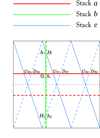
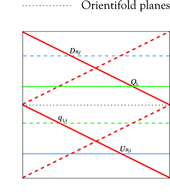
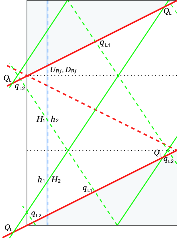
Figure 1: The configuration of D-brane stacks on the first, second, and third torus (from left to right). The stack $a$ is composed of 3 D6-branes, the stack $b$ of 2 D6-branes, and the stack $c$ is a single D6-brane. The broken lines and the dotted ones represent mirror branes and orientifold planes, respectively. Since D$6_{d}$-branes are not used for our analysis on quark sectors, they are not depicted. On the second torus, the open strings stretching between $b$-$c^{*}$ and $b$-$c$ correspond to the $H_{i}$’s, and the $h_{i}$’s. On the third torus, the unshaded portion is a fundamental region.

3 The intersecting brane model with a warp effect

We now show that a warp effect plays an important role in generating hierarchically suppressed fermion masses and CKM mixings. First, let us consider the up-quark sector. We define $A_{U,ij}^{(n)}$ as the area of a triangle formed by three intersection points $Q_{Li}$, $U_{Rj}$ and $X_{U,i}$ on the $n$-th torus, where $Q_{Li}=q_{i}\;(i=1,2)$, $Q_{L3}=Q_{L}$, $X_{U,i}=h_{1}\;(i=1,2)$ and $X_{U,3}=H_{1}$.

Then the Yukawa matrix for the up sector is described as $Y_{U,ij}=\langle X_{U,i}\rangle e^{-kA_{U,ij}}$, where $A_{U,ij}=A_{U,ij}^{(1)}+A_{U,ij}^{(3)}$. If there is no warping, owing to the degeneracy of the locations of quark doublets on the first torus, $A_{U,ij}^{(1)}$ depends only on the index $j$, where let us call it $A^{U}_{j}$. On the other hand, on the third torus the right handed quarks stay at the same point, thus we define $A^{Q}_{i}=A_{U,ij}^{(3)}$. Therefore, the Yukawa matrix for up-sector quarks is described as

$$Y_{U,ij}=\langle X_{U,i}\rangle a_{i}b^{U}_{j}$$ (3.15)

where $a_{i}=e^{-kA^{Q}_{i}}$ and $b^{U}_{j}=e^{-kA^{U}_{j}}.$ For the down-quark sector, we obtain

$$Y_{D,ij}=\langle X_{D,i}\rangle a_{i}b^{D}_{j}$$ (3.16)

where $b^{D}_{j}=e^{-kA^{D}_{j}}$, and $A^{D}_{j}$ is the area formed by $Q_{Li}$, $D_{Rj}$ and $X_{D,i}$ on the first torus, where $X_{D,i}=h_{2}\;(i=1,2)$ and $X_{D,3}=H_{2}$. For simplicity, we assume all the vacuum expectation values of Higgs fields to be unity throughout this paper.

This matrix cannot reproduce the realistic structure of CKM matrix and quark masses although it seems roughly consistent with them. Since this matrix is singular, we cannot have a definite unitary matrix diagonalizing $Y\cdot Y^{\dagger}$. In addition, the resultant CKM mixing matrix does not have any mixing between the third generation and the other ones. Besides, only one of three eigenvalues is non-zero for each sector, which means that the model cannot explain the masses of quarks and leptons except for the third generation. As for this problem, several attempts have been done for generating definite non-zero mixings. For example, the authors in Ref. [20, 21] argue on the basis of supersymmetric composite models constructed in the framework of intersecting brane model. The authors in Ref. [26] study the CKM mixing matrix in the model with 3 supersymmetric Higgs doublets, where all the matter fields arise from one of the tori.

Let us assume here that the metric of the first torus depends on a coordinate on the third torus $x_{8}$. Then, the length of strings projected on the first torus become dependent on the coordinate $x_{8}$, and so does the area swept by the strings. In this case, Yukawa couplings cannot be expressed in the simple form (3.15). In a rough approximation, we take the effect of the $x_{8}$-dependence into consideration by modifying $A^{(1)}_{j}$

$$A^{U}_{j}\rightarrow A^{U}_{j}(1-\epsilon_{i}),$$ (3.17)

where $\epsilon_{i}$ is a small quantity generated by the $x_{8}$-dependence. The $\epsilon_{i}$ is, in principle, calculable in string theory, but we treat them simply as input parameters. In this estimation, Yukawa couplings are no longer of the form (3.15), and thus Yukawa matrices would generically become non-degenerate. Surprisingly, this slight modification gives the realistic hierarchical structure of fermion masses and a CKM mixing matrix. In this paper, we attribute the $x_{8}$-dependence of the metric to a warp effect of the background geometry. Before calculating quark masses and CKM mixings, we here make a comment on the possibility of the emergence of warping in the intersecting brane model introduced in the previous section.

The warped geometry was first proposed in Ref. [30], where the authors began with a five dimensional model $M^{4}\times S^{1}/Z_{2}$, with cosmological constants in the 5D bulk space and on the 4D boundaries, and found a solution of the Einstein equation which shows that the 4D metric depends on the extra dimensional coordinate $\phi$: $ds^{2}=e^{-2kr_{c}|\phi|}\eta_{\mu\nu}dx^{\mu}dx^{\nu}+r^{2}_{c}d\phi^{2}$, where $k$ is a five dimensional scale and $r_{c}$ is the compactification radius.

It must be noted that the warping comes from localization of the energy density. In our setup, the internal manifold is $T^{2}\times T^{2}\times T^{2}$ and orientifold planes are located at $x^{4}=0,\,\pi;\ x^{6}=0,\,\pi;\ x^{8}=0,\,\pi$, and D-brane stacks are wrapped on three cycles on the tori. For simplifying the situation, let us smear the D-branes and orientifold planes on the first and second torus, not smearing them on the third torus, and assume that the D-brane stacks projected on the third torus are all parallel to the orientifolds. Looking at this configuration neglecting all the extra dimensions except for $x^{8}$, one could regard it as the 5 dimensional model compactified on $S^{1}/Z_{2}$ with two negative tension branes and several positive tension branes. Because of the localization of the positive energy branes and the negative energy branes, it seems valid to assume the emergence of a warp factor depending on $x_{8}$ though it might be small.

In the present paper, we do not attempt to solve the metric background, but it is interesting to note that the authors in Ref. [32] investigated a similar setup. They consider 10 dimensional Type IIA string theory compactified on $S^{1}/Z_{2}$ with parallel 32 D8-branes and O8-branes. Assuming that $2n$ D8-branes are located on the top of the orientifold plane at $x_{9}=0$, and $32-2n$ D8-branes on the orientifold plane at $x_{9}=\pi R$, where $R$ is the radius of $S^{1}/Z_{2}$, they found the solution

$$ds^{2} = H^{-1/2}_{\rm D8}[-dt^{2}+(dx^{\mu})^{2}]+H^{1/2}_{\rm D8}(dx^{9})^{2},$$ (3.18)

where $H_{\rm D8}=1-h_{\rm D8}|x^{9}|,\;h_{\rm D8}=\frac{(n-8)g_{s}}{2\pi l_{s}}$, $g_{s}$ is the string coupling constant, and $l_{s}=\sqrt{\alpha^{\prime}}$ is the string length. If we compactify this configuration on tori and T-dualize it twice, it becomes close to our model. Although the procedure of torus compactification might have an influence on the warp factor in (3.18), it is not so audacious to expect in our setup some kind of warping along one of the internal coordinates.

Now let us move to the evaluation of Yukawa matrices and calculate the CKM mixing matrix. Turning on the warp effect, we have Yukawa matrices for the up-sector:

$$Y^{U}_{ij} = e^{-kA^{U}_{ij}},$$ (3.19)

$$A^{U}_{ij} = A^{Q}_{i}+A^{U}_{j}(1-x\,c_{i}).$$ (3.20)

In this expression, we put $\epsilon_{i}$ in the form $\epsilon_{i}=xc_{i}$, where $x\ll 1$ and $c_{i}$ is of order 1 since the order of $\epsilon_{i}$ is thought to be of the same order. In order to calculate the masses and the CKM matrix on the basis of series expansion, besides $x$, we define two more small quantities $y$ and $z$ as

$$y=\frac{e^{-kA_{2}}}{e^{-kA_{3}}},\quad z=\frac{e^{-kA_{1}}}{e^{-kA_{2}}},\quad(A_{1}>A_{2}>A_{3}).$$ (3.21)

Solving the eigensystem of Yukawa matrices by series expansion with respect to $x$, $y$ and $z$, we finally obtain the leading part of up- and down- quark masses

$$m_{U/D,1}^{2} = \frac{2}{9}\beta^{U/D}_{4}\left\{(c^{U/D}_{3})^{4}+(c^{U/D}_{2})^{4}y^{2}\right\}x^{4},$$ (3.22)

$$m_{U/D,2}^{2} = \beta^{U/D}_{0}\alpha^{U/D}(c^{U/D}_{2}-c^{U/D}_{3})^{2}y^{2}x^{2},$$ (3.23)

$$m_{U/D,3}^{2} = \beta^{U/D}_{0}(1+y^{2}),$$ (3.24)

and the CKM mixing matrix

$$V_{\rm CKM} \sim \left(\matrix{1+\frac{{n_{4}}\,\left({n_{2}}+{n_{3}}\,x\right)}{2\,\alpha^{U}\alpha^{D}\,{\Delta^{D}_{23}}\,{{\Delta^{U}_{23}}}}\,z^{2}&n_{4}z-\frac{{n_{3}}}{2\alpha^{U}\alpha^{D}\Delta^{D}_{23}\,\Delta^{U}_{23}}\,xz&-\frac{\beta^{D}_{1}\,{n_{1}}}{\Delta^{U}_{23}}\,x\,y\,z\cr-n_{4}z+\frac{{n_{3}}}{2\alpha^{U}\alpha^{D}\Delta^{D}_{23}\,\Delta^{U}_{23}}\,xz&1+\frac{{n_{4}}\,\left({n_{2}}+{n_{3}}\,x\right)}{2\,\alpha^{U}\alpha^{D}\,{\Delta^{D}_{23}}\,{\Delta^{U}_{23}}}\,z^{2}&-{n_{5}}\,x\,y\cr\frac{\beta^{U}_{1}\,{n_{1}}}{{\Delta^{D}_{23}}}\,x\,y\,z&{n_{5}}\,x\,y&1\cr}\right),$$ (3.25)

where we define

$$n_{1} = c^{D}_{3}\Delta^{U}_{12}+c^{D}_{1}\Delta^{U}_{23}+c^{D}_{2}\Delta^{U}_{31},$$ (3.26)

$$n_{2} = -\alpha^{U}\alpha^{D}(\Delta^{D}_{31}\Delta^{U}_{23}-\Delta^{D}_{23}\Delta^{U}_{31}),$$ (3.27)

$$n_{3} = (\beta^{D}_{3}-\beta^{D}_{1}\beta^{D}_{2})\alpha^{U}\Delta^{D}_{12}\Delta^{D}_{31}\Delta^{U}_{23}-\alpha^{D}(\beta^{U}_{3}-\beta^{U}_{1}\beta^{U}_{2})\Delta^{D}_{23}\Delta^{U}_{12}\Delta^{U}_{31},$$ (3.28)

$$n_{4} = \frac{\Delta^{D}_{31}\Delta^{U}_{23}-\Delta^{D}_{23}\Delta^{U}_{31}}{\Delta^{D}_{23}\,\Delta^{U}_{23}},$$ (3.29)

$$n_{5} = -\beta^{D}_{1}\Delta^{D}_{23}+\beta^{U}_{1}\Delta^{U}_{23},$$ (3.30)

$$\Delta^{U}_{ij} = c^{U}_{i}-c^{U}_{j},\qquad\Delta^{D}_{ij}\;=\;c^{D}_{i}-c^{D}_{j},$$ (3.31)

$$\alpha^{U} = \beta^{U}_{2}-(\,\beta^{U}_{1}\,)^{2},\qquad\alpha^{D}\;=\;\beta^{D}_{2}-(\,\beta^{D}_{1}\,)^{2},$$ (3.32)

$$\beta^{U}_{0} = \sum_{j=1}^{3}(\,b^{U}_{j}\,)^{2},\qquad\beta^{D}_{0}\;=\;\sum_{j=1}^{3}(\,b^{D}_{j}\,)^{2},$$ (3.33)

$$\beta^{U}_{n} = \sum_{i=1}^{3}(\,b^{U}_{i}\,)^{2}\left(\log b^{U}_{i}\right)^{n}/\,\beta^{U}_{0},\qquad\beta^{D}_{n}\;=\;\sum_{i=1}^{3}(\,b^{D}_{i}\,)^{2}\left(\log b^{D}_{i}\right)^{n}/\,\beta^{D}_{0}$$ (3.34)

(for $$n=1,2,\cdots$$.)

If we ignore coefficients and assume $x$, $y$ and $z$ of order $\epsilon$, we can reproduce the hierarchical structure of the realistic CKM matrix:

$$V_{\rm CKM} \sim \left(\matrix{1-\epsilon^{2}&\epsilon&\epsilon^{3}\cr\epsilon&1-\epsilon^{2}&\epsilon^{2}\cr\epsilon^{3}&\epsilon^{2}&1}\right).$$ (3.35)

In this naïve estimation, the masses of the first and the second generations, $m_{1}\sim x^{2}$ and $m_{2}\sim xy$, turn out of the same order $\epsilon^{2}$, and one might regard it as an undesirable result. However, noting that $x$ comes from a small warp factor, and that it should be smaller than $y$ and $z$, the mass difference is expected to come from a small value of this ratio $x/y$ and, of course, from the coefficients we have so far neglected.

4 Discussion

In this paper, we propose a method for reproducing the realistic hierarchical structure of the observed quark masses and CKM mixing matrix on the basis of a specific intersecting brane model proposed in Ref. [9]. We newly introduced a small warp factor on tori, which systematically changes the elements of hierarchically suppressed but singular Yukawa matrices. The modification gives two hierarchically suppressed quark masses and that of order 1 in addition to a definite CKM mixing matrix. Taking the order of several parameters appropriately, we reproduce the realistic hierarchical structure of quark masses and a CKM mixing matrix. It is worth noting that both large mass hierarchy and small mixing angles are originated from a warp factor on the internal manifold.

Acknowledgments

The author is grateful to Masahiro Yamaguchi for valuable discussions and comments. The author also thanks the Japan Society for the Promotion of science for financial support.

References

- [1] J. Polchinski, “Dirichlet-Branes and Ramond-Ramond Charges,” Phys. Rev. Lett. 75, 4724 (1995) [arXiv:hep-th/9510017].
- [2] R. Blumenhagen, L. Görlich, B. Körs and D. Lüst, “Noncommutative compactifications of type I strings on tori with magnetic background flux,” JHEP 0010, 006 (2000) [arXiv:hep-th/0007024].
- [3] R. Blumenhagen, L. Görlich, B. Körs and D. Lüst, “Magnetic flux in toroidal type I compactifications,” Fortsch. Phys. 49, 591 (2001) [arXiv:hep-th/0010198].
- [4] R. Blumenhagen, B. Körs and D. Lüst, “Type I strings with F- and B-flux,” JHEP 0102, 030 (2001) [arXiv:hep-th/0012156].
- [5] M. Berkooz, M. R. Douglas and R. G. Leigh, “Branes intersecting at angles,” Nucl. Phys. B 480, 265 (1996) [arXiv:hep-th/9606139].
- [6] H. Arfaei and M. M. Sheikh Jabbari, “Different D-brane interactions,” Phys. Lett. B 394, 288 (1997) [arXiv:hep-th/9608167].
- [7] G. Aldazabal, S. Franco, L. E. Ibáñez, R. Rabadán and A. M. Uranga, “D = 4 chiral string compactifications from intersecting branes,” J. Math. Phys. 42, 3103 (2001) [arXiv:hep-th/0011073].
- [8] G. Aldazabal, S. Franco, L. E. Ibáñez, R. Rabadán and A. M. Uranga, “Intersecting brane worlds,” JHEP 0102, 047 (2001) [arXiv:hep-ph/0011132].
- [9] L. E. Ibáñez, F. Marchesano and R. Rabadán, “Getting just the standard model at intersecting branes,” JHEP 0111, 002 (2001) [arXiv:hep-th/0105155].
- [10] D. Cremades, L. E. Ibáñez and F. Marchesano, “Intersecting brane models of particle physics and the Higgs mechanism,” JHEP 0207, 022 (2002) [arXiv:hep-th/0203160].
- [11] D. Cremades, L. E. Ibáñez and F. Marchesano, “Yukawa couplings in intersecting D-brane models,” JHEP 0307, 038 (2003) [arXiv:hep-th/0302105].
- [12] C. Kokorelis, “GUT model hierarchies from intersecting branes,” JHEP 0208, 018 (2002) [arXiv:hep-th/0203187].
- [13] J. R. Ellis, P. Kanti and D. V. Nanopoulos, “Intersecting branes flip SU(5),” Nucl. Phys. B 647, 235 (2002) [arXiv:hep-th/0206087].
- [14] M. Cvetič, I. Papadimitriou and G. Shiu, “Supersymmetric three family SU(5) grand unified models from type IIA orientifolds with intersecting D6-branes,” Nucl. Phys. B 659, 193 (2003) [Erratum-ibid. B 696, 298 (2004)] [arXiv:hep-th/0212177].
- [15] M. Axenides, E. Floratos and C. Kokorelis, “SU(5) unified theories from intersecting branes,” JHEP 0310, 006 (2003) [arXiv:hep-th/0307255].
- [16] M. Cvetič, G. Shiu and A. M. Uranga, “Three-family supersymmetric standard like models from intersecting brane worlds,” Phys. Rev. Lett. 87, 201801 (2001) [arXiv:hep-th/0107143].
- [17] M. Cvetič, G. Shiu and A. M. Uranga, “Chiral four-dimensional N = 1 supersymmetric type IIA orientifolds from intersecting D6-branes,” Nucl. Phys. B 615, 3 (2001) [arXiv:hep-th/0107166].
- [18] M. Cvetič, P. Langacker and G. Shiu, “Phenomenology of a three-family standard-like string model,” Phys. Rev. D 66, 066004 (2002) [arXiv:hep-ph/0205252].
- [19] G. Honecker and T. Ott, “Getting just the supersymmetric standard model at intersecting branes on the Z(6)-orientifold,” arXiv:hep-th/0404055.
- [20] N. Kitazawa, “Supersymmetric composite models on intersecting D-branes,” arXiv:hep-th/0401096.
- [21] N. Kitazawa, T. Kobayashi, N. Maru and N. Okada, “Yukawa coupling structure in intersecting D-brane models,” arXiv:hep-th/0406115.
- [22] M. Cvetič, P. Langacker and G. Shiu, “A three-family standard-like orientifold model: Yukawa couplings and hierarchy,” Nucl. Phys. B 642, 139 (2002) [arXiv:hep-th/0206115].
- [23] M. Cvetič and I. Papadimitriou, “Conformal field theory couplings for intersecting D-branes on orientifolds,” Phys. Rev. D 68, 046001 (2003) [Erratum-ibid. D 70, 029903 (2004)] [arXiv:hep-th/0303083].
- [24] S. A. Abel and A. W. Owen, “Interactions in intersecting brane models,” Nucl. Phys. B 663, 197 (2003) [arXiv:hep-th/0303124].
- [25] D. Lüst, P. Mayr, R. Richter and S. Stieberger, “Scattering of gauge, matter, and moduli fields from intersecting branes,” Nucl. Phys. B 696, 205 (2004) [arXiv:hep-th/0404134].
- [26] N. Chamoun, S. Khalil and E. Lashin, “Fermion masses and mixing in intersecting branes scenarios,” Phys. Rev. D 69, 095011 (2004) [arXiv:hep-ph/0309169].
- [27] I. R. Klebanov and E. Witten, “Proton decay in intersecting D-brane models,” Nucl. Phys. B 664, 3 (2003) [arXiv:hep-th/0304079].
- [28] S. A. Abel, M. Masip and J. Santiago, “Flavour changing neutral currents in intersecting brane models,” JHEP 0304, 057 (2003) [arXiv:hep-ph/0303087].
- [29] S. A. Abel, O. Lebedev and J. Santiago, “Flavour in intersecting brane models and bounds on the string scale,” Nucl. Phys. B 696, 141 (2004) [arXiv:hep-ph/0312157].
- [30] L. Randall and R. Sundrum, “A large mass hierarchy from a small extra dimension,” Phys. Rev. Lett. 83, 3370 (1999) [arXiv:hep-ph/9905221].
- [31] E. Witten, “Strong Coupling Expansion Of Calabi-Yau Compactification,” Nucl. Phys. B 471, 135 (1996) [arXiv:hep-th/9602070].
- [32] E. Bergshoeff, R. Kallosh, T. Ortín, D. Roest and A. Van Proeyen, “New formulations of D = 10 supersymmetry and D8-O8 domain walls,” Class. Quant. Grav. 18, 3359 (2001) [arXiv:hep-th/0103233].
- [33] C. S. Chan, P. L. Paul and H. Verlinde, “A note on warped string compactification,” Nucl. Phys. B 581, 156 (2000) [arXiv:hep-th/0003236].