Implications for New Physics
from Fine-Tuning Arguments:
I. Application to SUSY and Seesaw Cases

We revisit the standard argument to estimate the scale of new physics (NP) beyond the SM, based on the sensitivity of the Higgs mass to quadratic divergences. Although this argument is arguably naive, the corresponding estimate, $\Lambda_{\rm SM}\stackrel{{\scriptstyle<}}{{{}_{\sim}}}2-3$ TeV, works reasonably well in most cases and should be considered a conservative bound, as it ignores other contributions to the Higgs mass which are potentially large. Besides, the possibility of an accidental Veltman-like cancellation does not raise significantly $\Lambda_{\rm SM}$. One can obtain more precise implications from fine-tuning arguments in specific examples of NP. Here we consider SUSY and right-handed (seesaw) neutrinos. SUSY is a typical example for which the previous general estimate is indeed conservative: the MSSM is fine-tuned a few %, even for soft masses of a few hundred GeV. In contrast, other SUSY scenarios, in particular those with low-scale SUSY breaking, can easily saturate the general bound on $\Lambda_{\rm SM}$. The seesaw mechanism requires large fine-tuning if $M_{R}\stackrel{{\scriptstyle>}}{{{}_{\sim}}}10^{7}$ GeV, unless there is additional NP (SUSY being a favourite option).

October 2004

IFT-UAM/CSIC-04-57

hep-ph/0410298

1 Introduction

It is commonly assumed that the Big Hierarchy Problem of the Standard Model (SM) indicates the existence of New Physics (NP) beyond the SM at a scale $\Lambda_{\rm SM}\stackrel{{\scriptstyle<}}{{{}_{\sim}}}$ few TeV. The argument is quite simple and well known. In the SM (treated as an effective theory valid below $\Lambda_{\rm SM}$) the mass parameter in the Higgs potential, $m^{2}$, receives important quadratically-divergent contributions. At one-loop [1],

$$\delta_{\rm q}m^{2}={3\over 64\pi^{2}}(3g^{2}+g^{\prime 2}+8\lambda-8\lambda_{t}^{2})\Lambda_{\rm SM}^{2}\ ,$$ (1)

where $g,g^{\prime},\lambda$ and $\lambda_{t}$ are the $SU(2)\times U(1)_{Y}$ gauge couplings, the quartic Higgs coupling and the top Yukawa coupling respectively. In terms of masses

$$\delta_{\rm q}m^{2}={3\over 16\pi^{2}v^{2}}(2m_{W}^{2}+m_{Z}^{2}+m_{h}^{2}-4m_{t}^{2})\Lambda_{\rm SM}^{2}\ ,$$ (2)

where $m_{W}^{2}=g^{2}v^{2}/4$, $m_{Z}^{2}=(g^{2}+g^{\prime 2})v^{2}/4$, $m_{h}^{2}=2\lambda v^{2}$ and $m_{t}^{2}=\lambda_{t}^{2}v^{2}/2$, with $v=246$ GeV. Upon minimization of the potential, this translates into a dangerous contribution to the Higgs vacuum expectation value (VEV) which tends to destabilize the electroweak scale. The requirement of no fine-tuning between the above contribution and the tree-level value of $m^{2}$ sets an upper bound on $\Lambda_{\rm SM}$. E.g. for $m_{h}=115-200$ GeV

$$\left|{\delta_{\rm q}m^{2}\over m^{2}}\right|=\left|{\delta v^{2}\over v^{2}}\right|\leq 10\ \Rightarrow\ \Lambda_{\rm SM}\stackrel{{\scriptstyle<}}{{{}_{\sim}}}2-3\ {\rm TeV}\ ,$$ (3)

where we have used $m_{h}^{2}=2m^{2}$ [valid in the approximation of disregarding terms beyond ${\cal O}(h^{4})$ in the Higgs potential]. This upper bound on $\Lambda_{\rm SM}$ is in a certain tension with bounds on the suppression scale of higher order operators derived from fits to precision electroweak data [2], which require $\Lambda\stackrel{{\scriptstyle>}}{{{}_{\sim}}}$ 10 TeV or even higher for some particularly dangerous operators (e.g. if they are flavour non-conserving). This is known as the “Little Hierarchy” problem, and implies that the NP at $\Lambda_{\rm SM}$ should be “clever” enough to be consistent with these constraints, giving some hints about its properties. E.g. non-strongly-interacting, flavour-blind NP is favoured.

The previous “Big Hierarchy” argument leads to an optimistic prospect, as it sets the scale of NP on the reach of LHC. However, as stressed in ref. [3], $\Lambda_{\rm SM}$ could be much larger if the Higgs mass lies (presumably by accident) close to the value that cancels $\delta_{\rm q}m^{2}$ in (2). At one-loop this is the famous Veltman’s condition [1]

$$2m_{W}^{2}+m_{Z}^{2}+m_{h}^{2}-4m_{t}^{2}\simeq 0\ ,$$ (4)

which is fulfilled for $m_{h}\simeq 307$ GeV . At higher order the condition becomes cut-off dependent [5]

$$\sum_{n\geq 0}c_{n}(\lambda_{i})\log^{n}{\Lambda\over m_{h}}\simeq 0\ ,$$ (5)

where $\lambda_{i}$ are the couplings of the SM and $c_{0}(\lambda_{i})=(3g^{2}+g^{\prime 2}+8\lambda-8\lambda_{t}^{2})$, the combination that appears in the one-loop Veltman correction. Eq. (5) is nothing but $c_{0}(\lambda_{i})$ evaluated at the cut-off scale $\Lambda$ and therefore contains the leading-log corrections to all orders. However, it does not include subleading (finite and next-to-leading-log) contributions which are not important for moderate values of $\Lambda$ [3]. The results of ref. [3], obtained by working at two-loop leading-log, are summarized in the fig. 2 of that paper, which is similar to our fig. 1, to be discussed in the next section. There, the lines of 10% and 1% fine-tuning show a throat (sometimes called “Veltman’s throat”), which corresponds to eq. (5). More precisely, the plot indicates that if $m_{h}\sim 210-225$ GeV, $\Lambda_{\rm SM}$ could be $\stackrel{{\scriptstyle>}}{{{}_{\sim}}}10$ TeV with no fine-tuning price and no Little Hierarchy problem. Incidentally, this solution would be far more economic than Little Higgs models [6]. (Likewise, a Little Higgs model with $m_{h}$ in the above range would lack genuine motivation.) On the negative side, this means that if $m_{h}$ is in this range, NP might escape detection at LHC.

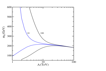
Figure 1: Fine-tuning contours corresponding to $\Delta_{\Lambda}=10$ and 100, i.e. 10% and 1% fine-tuning, respectively.

In this paper we re-examine the use of the Big Hierarchy Problem of the SM to extract information about the size of $\Lambda_{\rm SM}$, illustrating our general results with physically relevant examples.

In section 2 we consider the possibility of living near a Veltman’s condition. In contrast with previous discussions in the literature, we show that this potential circumstance does not reduce the amount of fine-tuning (once it is evaluated in a complete way), so that the upper bound on $\Lambda_{\rm SM}$ is not affected much at present.

In section 3, we examine the limitations of the Big Hierarchy argument to estimate the scale of new physics. We argue that the reasoning, as usually presented and summarized above, is too naive. However, quantitatively, the corresponding estimate for the upper bound on $\Lambda_{\rm SM}$ turns out to work reasonably well in most cases, and, indeed, it should be considered a conservative bound, as it ignores potentially large contributions to the Higgs mass parameter.

In section 4, we analyze two physically relevant examples of NP: right-handed (seesaw) neutrinos and supersymmetry (SUSY). We discuss how, in the context of the SM, the seesaw mechanism produces a very important fine-tuning problem which claims for the existence of additional NP. On the other hand SUSY illustrates the fact that the “naive” bound is indeed conservative. E.g. the MSSM is quite fine-tuned even for soft masses of a few hundred GeV. We discuss how other SUSY scenarios, in particular those with low-scale SUSY breaking, can easily evade the problematic aspects of the MSSM, essentially saturating the general bound.

Another example of new physics, namely Little Higgs models, deserve a separate analysis and will be the subject of a companion paper.

Finally, we summarize and present our conclusions in section 5.

2 Remarks on the shape of Veltman’s throat

We start our analysis by re-examining the argument that led to the expectation of a fine-tuning throat, as presented in the previous section. To quantify the tuning we follow Barbieri and Giudice [7]: we write the Higgs VEV as $v^{2}=v^{2}(p_{1},p_{2},\cdots)$, where $p_{i}$ are initial parameters of the model under study, and measure the amount of fine tuning associated to $p_{i}$ by $\Delta_{p_{i}}$, defined as

$${\delta M_{Z}^{2}\over M_{Z}^{2}}={\delta v^{2}\over v^{2}}=\Delta_{p_{i}}{\delta p_{i}\over p_{i}}\ ,$$ (6)

where $\delta M_{Z}^{2}$ (or $\delta v^{2}$) is the change induced in $M_{Z}^{2}$ (or $v^{2}$) by a change $\delta p_{i}$ in $p_{i}$. Roughly speaking $\Delta^{-1}_{p_{i}}$ measures the probability of a cancellation among terms of a given size to obtain a result which is $\Delta_{p_{i}}$ times smaller.

The discussion of the previous section concerns the dependence of $v^{2}$ on the scale $\Lambda_{\rm SM}$. Indeed, plotting the lines of $\Delta_{\Lambda}=$ 10, 100 in the ($m_{h},\Lambda$) plane, as shown in fig. 1, we obtain curves similar to the 10% and 1% curves in fig. 2 of ref. [3], as discussed in the Introduction, reproducing the throat already mentioned.

Our first remark has to do with the fact that, besides $\Lambda$, there are other relevant parameters which are not yet measured with extreme precision. The most notable case is the top mass, which, according to the latest experimental data [8], is

$$M_{t}=178\pm 4.3\ {\rm GeV}\ .$$ (7)

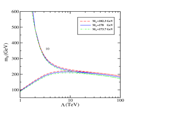
Figure 2: Same as fig. 1 for $\Delta_{\Lambda}=10$ and three different values of the top mass.

Although this uncertainty is remarkably small, it should not be ignored for fine-tuning issues. Figure 2 shows three curves with $\Delta_{\Lambda}=$ 10, corresponding to $M_{t}=$ 173.7, 178 and 182.3 GeV. The value of $\Delta_{\Lambda}$ should be averaged over all the allowed ranges of variation of the unknown parameters, and in this case this averaging has the effect of cutting the throat at $\Lambda\simeq 10$ TeV. This is characteristic of fine-tuning arguments: since they are based on statistical considerations, the conclusions may vary according to our partial (and time-dependent) knowledge of the relevant parameters in the problem. An alternative way of taking into account the uncertainty in $\Lambda$ and $M_{t}$ simultaneously is to add $\Delta_{\Lambda}$ and $\Delta_{\lambda_{t}}$ in quadrature (where the running top mass is $m_{t}=\lambda_{t}v/\sqrt{2}$):

$$\Delta=\left(\Delta_{\Lambda}^{2}+\Delta_{\lambda_{t}}^{2}\right)^{1/2}\ .$$ (8)

Since $\lambda_{t}$ should only vary within the experimentally allowed range, we modify the definition of $\Delta_{\lambda_{t}}$ as

$$\Delta_{\lambda_{t}}={\partial v^{2}\over\partial\lambda_{t}}{\lambda_{t}\over v^{2}}\times{\delta^{\rm exp}\lambda_{t}\over\lambda_{t}}\ ,$$ (9)

(see ref. [9] for a discussion of this point). In figure 3 (left plot), which shows the $\Delta=$ 10, 100 curves, we indeed see a cut at $\Lambda\simeq 10$ TeV for $\Delta=$ 10. All this means that, in the absence of any theoretical reason to be at Veltman’s throat, or of precision measurements showing that we are really there, fine-tuning arguments put an upper limit on the value of $\Lambda_{\rm SM}$.

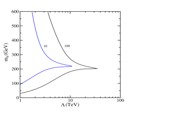
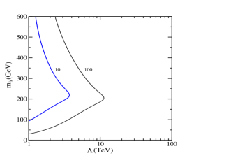
Figure 3: Contour plots of $\Delta=10,100$. Left: with $\Delta$ as defined in eqs. (8, 9). Right: with $\Delta$ as defined in eq. (10).

Our second remark concerns the fact that $m_{h}$ itself (and thus the quartic Higgs coupling, $\lambda$) is not known at present. Therefore the previous results, in particular the left plot in fig. 3, correspond to a future time when $m_{h}$ will be known. For instance, if LEP’s inconclusive evidence for $m_{h}\simeq 115$ GeV [10] gets confirmed, then one expects $\Lambda_{\rm SM}\stackrel{{\scriptstyle<}}{{{}_{\sim}}}1.4$ TeV. At present one should average all the possible values of $m_{h}^{2}$, say in the range 115 GeV $\leq m_{h}\leq$ 600 GeV, which gives the result $\Lambda_{\rm SM}\stackrel{{\scriptstyle<}}{{{}_{\sim}}}2.5$ TeV. Again, we can alternatively add in quadrature $\Delta_{\lambda}$ to obtain the global fine-tuning,

$$\Delta=\left(\Delta_{\Lambda}^{2}+\Delta_{\lambda_{t}}^{2}+\Delta_{\lambda}^{2}\right)^{1/2}\ .$$ (10)

The corresponding curve for $\Delta=$ 10 is shown in the right plot of fig. 3, which corresponds to the present status of the problem. $\Lambda_{\rm SM}$ depends slightly on $m_{h}$, being always below 4 TeV. In average, $\Lambda_{\rm SM}^{\rm av}\stackrel{{\scriptstyle<}}{{{}_{\sim}}}2.5$ TeV.

3 Limitations of the use of the hierarchy problem to estimate ${\mbox{\boldmath{$\Lambda$}}}_{\rm{\bf SM}}$

Besides the previous subtleties about the shape of Veltman’s throat, there are more general caveats about using the hierarchy problem to estimate the scale of new physics. The argument, as usually presented and summarized in the Introduction, implicitly assumes that the job of the new physics is to cancel the dangerous contributions of the SM diagrams for momenta above $\Lambda_{\rm SM}$, leaving uncancelled the quadratically divergent contributions evaluated in the SM and cut off at $\Lambda_{\rm SM}$ (except for artificial tunings or fortunate accidents). However, the effects of the new physics do not enter in such an abrupt and sharp way. Generically, the new diagrams give a non-negligible contribution already below $\Lambda_{\rm SM}$, and do not cancel exactly the SM contributions above $\Lambda_{\rm SM}$ . Remnants of this imperfect cancellation are finite and logarithmic contributions from NP, which are not simply given by the SM divergent part cut off at $\Lambda_{\rm SM}$. The familiar example is SUSY, where the cancellation of the quadratically divergent contributions between the SM and the NP particles automatically occurs for all momenta, even after the breaking of SUSY. If the only problem were this type of contributions, the scale of SUSY breaking (and thus $\Lambda_{\rm SM}$) could be as large as desired. Of course, this is not so because of the presence of other dangerous logarithmic and finite contributions to the Higgs mass parameter, $m^{2}$, from superpartners. For instance, the stop sector, $\tilde{t}$, contributes

$$\delta m^{2}=-{3\lambda_{t}^{2}\over 8\pi^{2}}m_{\tilde{t}}^{2}\log{\Lambda^{2}\over m_{\tilde{t}}^{2}}\ .$$ (11)

This contribution does not cancel if SUSY is broken, setting finally the bound $\Lambda_{\rm SM}\simeq m_{\tilde{t}}\stackrel{{\scriptstyle<}}{{{}_{\sim}}}$ few hundred GeV.

The supersymmetric example clearly shows that Veltman’s condition may be irrelevant for estimating $\Lambda_{\rm SM}$. In SUSY the quadratically-divergent contributions to $m^{2}$ are cancelled anyway, with or without Veltman’s condition; but there are dangerous contributions from new physics, which do not cancel (in principle), and are totally unrelated to Veltman’s condition.

The previous discussion can be generalized in a straightforward way. For this matter, it is convenient to write the general one-loop effective potential using a momentum cut-off regularization, $V=V_{0}+V_{1}+\cdots$ , with

$$V_{0}={1\over 2}m^{2}h^{2}+{1\over 4}\lambda h^{4}\ ,$$ (12)

$$V_{1}={1\over 64\pi^{2}}{\rm Str}\left[2\Lambda^{2}{\cal M}^{2}+{\cal M}^{4}\left(\log{{\cal M}^{2}\over\Lambda^{2}}-{1\over 2}\right)\right]+{\cal O}\left({{\cal M}^{6}\over\Lambda^{2}}\right)\ ,$$ (13)

where $h$ is the (real and neutral) Higgs field, the supertrace ${\rm Str}$ counts degrees of freedom with a minus sign for fermions, and ${\cal M}^{2}$ is the (tree-level, $h-$dependent) mass-squared matrix. The one-loop contribution to the Higgs mass parameter is

$$\delta_{1}m^{2} = \left.{\partial^{2}V_{1}\over\partial h^{2}}\right|_{h=0}$$ (14)

$$= {1\over 32\pi^{2}}{\rm Str}\left[{\partial^{2}{\cal M}^{2}\over\partial h^{2}}\left(\Lambda^{2}+{\cal M}^{2}\log{{\cal M}^{2}\over\Lambda^{2}}\right)+\left({\partial{\cal M}^{2}\over\partial h}\right)^{2}\left(\log{{\cal M}^{2}\over\Lambda^{2}}+1\right)\right]_{h=0}.$$

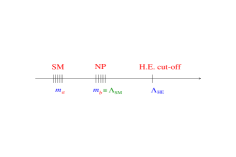
Figure 4: Schematic representation of the spectra associated to the various scales of the theory: Standard Model (SM), New Physics (NP) beyond the Standard Model and the high energy cut-off.

We will now separate the supertraces as sums over SM and NP states. The masses of the (lightest) NP states act as the effective SM cut-off, $\Lambda_{\rm SM}$, but it is convenient to consider the possible existence of a High-Energy cut-off , $\Lambda_{\rm HE}$, since the NP may not be yet the truly fundamental theory. This is schematically represented in fig. 4. $\Lambda_{\rm HE}$ can be as large as the Planck scale or much lower, close to the masses of the NP states. Then

$$\delta_{1}m^{2} = {1\over 32\pi^{2}}\sum_{a}^{\small\rm SM}N_{a}\left[{\partial^{2}m_{a}^{2}\over\partial h^{2}}\left(\Lambda^{2}+m_{a}^{2}\log{m_{a}^{2}\over\Lambda^{2}}\right)\right]_{h=0}$$ (15)

$$+ {1\over 32\pi^{2}}\sum_{b}^{\small\rm NP}N_{b}\left[{\partial^{2}m_{b}^{2}\over\partial h^{2}}\left(\Lambda^{2}+m_{b}^{2}\log{m_{b}^{2}\over\Lambda^{2}}\right)+\left({\partial m_{b}^{2}\over\partial h}\right)^{2}\left(\log{m_{b}^{2}\over\Lambda^{2}}+1\right)\right]_{h=0},$$

where $m_{a},N_{a}$ ($m_{b},N_{b}$) represent the mass and multiplicity, with negative sign for fermions, of the SM (NP) states, and $\Lambda\equiv\Lambda_{\rm HE}$. From the SM contributions, only the quadratically divergent ones are dangerous. The other terms are vanishing, except for the contribution of the Higgs field itself, which is not large. On the other hand, all NP contributions (quadratic, logarithmic and finite) are potentially dangerous. Now several situations might take place:

i)

There are no special cancellations among the different contributions in eq. (15). In that case the simple (Big Hierarchy) argument, based on the size of the quadratic contributions, and the corresponding bound $\Lambda\stackrel{{\scriptstyle<}}{{{}_{\sim}}}2-3$ TeV, apply. The argument is clearly a conservative one due to the presence of extra contributions, which are discussed below.

ii)

The SM quadratically divergent contributions cancel (maybe approximately) by themselves, i.e. they are close to Veltman’s condition. This is the situation discussed in the previous section. There we saw that, in the absence of a fundamental reason for the exact cancellation, one expects NP not far from the TeV scale (“Veltman’s throat” is always cut). But, clearly the new states re-introduce the problem [second line of eq. (15)]: even if these new states do not give new quadratically divergent contributions, fine-tuning considerations require also $m_{b}\equiv\Lambda_{\rm SM}\stackrel{{\scriptstyle<}}{{{}_{\sim}}}2-3$ TeV, as discussed next.

iii)

The SM and NP quadratically divergent contributions cancel each other, i.e.

$$\sum_{a}^{\small\rm SM}N_{a}\left.{\partial^{2}m_{a}^{2}\over\partial h^{2}}\right|_{h=0}+\sum_{b}^{\small\rm NP}N_{b}\left.{\partial^{2}m_{b}^{2}\over\partial h^{2}}\right|_{h=0}=0\ .$$ (16)

This occurs naturally in SUSY and little-Higgs models. But, again, the logarithmic and finite NP contributions in eq. (15) are also dangerous and, as in case ii), re-introduce the problem, albeit in a softer form. Notice also that these contributions (unlike the quadratic ones) show up in any regularization scheme, differing only in the value of the finite pieces. For future use, we write them in the $\overline{\rm MS}$ scheme

$$\delta_{\rm NP}^{\overline{\rm MS}}\ m^{2}=\sum_{b}^{\small\rm NP}{N_{b}\over 32\pi^{2}}\left[{\partial^{2}m_{b}^{2}\over\partial h^{2}}m_{b}^{2}\left(\log{m_{b}^{2}\over Q^{2}}-1\right)+\left({\partial m_{b}^{2}\over\partial h}\right)^{2}\log{m_{b}^{2}\over Q^{2}}\right]_{h=0}\ ,$$ (17)

where $Q$ is the renormalization scale, to be identified with the cut-off scale, $\Lambda$. Quantitatively, these contributions are roughly similar to the SM quadratically-divergent one, replacing $\Lambda\rightarrow m_{b}\equiv\Lambda_{\rm SM}$. This gives the basis for the estimate of the “naive” Big Hierarchy argument discussed in the Introduction. However, new parameters not present in the SM might enter through the $m_{b}$ masses and, moreover, the presence of the logarithmically-enhanced terms makes the new contributions typically more dangerous than the SM estimate (as happens for instance in the supersymmetric case commented above). Hence, from fine-tuning arguments we can keep $m_{b}\equiv\Lambda_{\rm SM}\stackrel{{\scriptstyle<}}{{{}_{\sim}}}2-3$ TeV, as a conservative bound.

Of course, if the NP is itself an effective theory derived from a more fundamental one, further extra states [which could have ${\cal O}(M_{p})$ masses] would be even more dangerous, unless their contributions are under control for some reason. The only clear example of this desirable property occurs when the theory is supersymmetric.

iv)

It may happen that, besides the cancellation of quadratic contributions, the other dangerous contributions also cancel or are absent. In the $\overline{\rm MS}$ scheme this means that eq. (17) vanishes. This could happen by accident or for some fundamental reason. In either case, the scale of new physics could be really much larger than a few TeV. The obvious remark is that no such fundamental reason is known. In its absence, one has to average over the possible ranges of variation of the parameters defining the new physics (e.g. the soft masses for the MSSM). In this way the usual result $\Lambda_{\rm SM}\stackrel{{\scriptstyle<}}{{{}_{\sim}}}2-3$ TeV is generically recovered.

To be on the safe side, however, one should not disregard completely the possibility that eq. (17) could be vanishing, which would allow for a very large $\Lambda_{\rm SM}$. It is fun to imagine some scenarios of this kind. E.g. if the NP states get masses through conventional Yukawa couplings (this is the case of a fourth generation), eq. (17) vanishes. Notice that, strictly speaking, those extra states do not represent a genuine new scale of physics as their masses arise from the electroweak breaking scale. In any case, the cancellation of the quadratic divergences would require to be close to a (modified) Veltman’s condition, and the discussion of point ii) above would follow. In addition, a heavy fourth generation would have problems of perturbativity and stability of the Higgs potential, among others. Another possibility is that the SM is close to Veltman’s condition and the new physics corresponds to heavy supersymmetric representations [possibly plus ${\cal O}({\rm TeV})$ soft breaking terms] (such partially-supersymmetric models have been already considered in the context of extra dimensions [12]). A further possibility will be discussed at the end of sect. 4.

Although the previous examples do not seem realistic, it is not unconceivable that the unknown fundamental physics is smart enough to implement naturally a cancellation of eq. (17), as SUSY does with the quadratic divergences. In that case fine-tuning arguments would be misleading.

Leaving aside the last caveats, it follows from the previous discussion that the “naive” procedure to estimate the scale of NP, by considering the SM quadratically-divergent contribution with $\Lambda\rightarrow\Lambda_{\rm SM}$, works reasonably well in most cases. Actually it is a conservative one, since it disregards unknown contributions that tend to be larger. On the other hand, it is not reliable to make more detailed statements based on this argument. In particular, the conditions for the cancellation (or quasi-cancellation) of the SM dangerous contributions are in principle unrelated to the cancellation of the unknown dangerous contributions. At this point the effective theory is unable to provide information about the dangers of the new physics.

Therefore, to derive more accurate implications for new physics from fine-tuning arguments, one should consider specific possibilities for physics beyond the SM. We examine two relevant examples in the rest of the paper.

4 Examples of New Physics

4.1 Right-handed seesaw neutrinos

The simplest extension of the ordinary SM is obtained by adding right-handed neutrinos, $\nu_{R}$ (one per family). The usual goal is to describe neutrino masses, either by conventional Yukawa couplings or through a seesaw mechanism. The latter is probably the most elegant mechanism to explain the smallness of neutrino masses. Then, the SM Lagrangian is simply enlarged with

$${\cal L}_{\nu}=-\nu_{R}m_{D}\nu_{L}-{1\over 2}\nu_{R}M_{R}\nu_{R}^{T}+{\rm h.c.}\ ,$$ (18)

where $m_{D}$ is the Dirac mass matrix ($m_{D}=-\lambda_{\nu}h/\sqrt{2}$, where $\lambda_{\nu}$ is the neutrino Yukawa coupling, a matrix in flavour space) and $M_{R}$ is the Majorana mass matrix for right-handed neutrinos. For our purposes it is enough to consider a single neutrino species, so that the above matrices reduce to numbers. For $M_{R}^{2}\gg m_{D}^{2}$, the two mass-squared eigenvalues are

$$m_{\nu_{1}}^{2} = {m_{D}^{4}\over M_{R}^{2}}+{\cal O}\left({m_{D}^{6}\over M_{R}^{4}}\right)\ ,$$

$$m_{\nu_{2}}^{2} = M_{R}^{2}+2m_{D}^{2}+{\cal O}\left({m_{D}^{4}\over M_{R}^{2}}\right)\ .$$ (19)

The lightest eigenstate is part of the effective low-energy theory and does not contribute radiatively to the Higgs mass parameter, as it is apparent from eq. (15). The heaviest one, however, contributes not only to the quadratic divergence, but also to the finite and logarithmic parts of $\delta_{1}m^{2}$:

$$\delta_{\nu}m^{2}=-{\lambda_{\nu}^{2}\over 16\pi^{2}}\left[2\Lambda^{2}+2M_{R}^{2}\log{M_{R}^{2}\over\Lambda^{2}}\right]\ .$$ (20)

This equation is a particularly simple example of the second line of eq. (15) and illustrates the general discussion of the previous section. In particular, even if the quadratically divergent contributions of the SM cancel the one of eq. (20) (which, incidentally, means that Veltman’s condition is modified by undetectable physics), there are other dangerous contributions which do not cancel. In other words, this represents a new manifestation of the hierarchy problem [13] since a cancellation between the quadratic and the logarithmic and finite contributions would be completely artificial and depends on the choice of renormalization scheme.

The logarithmic and finite contributions are especially disturbing as their size is associated to $M_{R}$ (which is expected to be very large) and show up in any renormalization scheme. In the $\overline{\rm MS}$ scheme [see eq. (17)]

$$\delta_{\nu}^{\overline{\rm MS}}m^{2}=-{\lambda_{\nu}^{2}\over 8\pi^{2}}M_{R}^{2}\left[\log{M_{R}^{2}\over\Lambda^{2}}-1\right]\ ,$$ (21)

where we have already set $Q=\Lambda$. Now it is easy to obtain a lower bound on the size of $M_{R}$ from the request of no fine-tuning. Demanding

$$\left|{\delta_{\nu}m^{2}\over m^{2}}\right|\leq\Delta\ ,$$ (22)

requires

$$M_{R}<10^{7}\ {\rm GeV}\ \Delta^{1/3}\left({m_{h}\over 200\ {\rm GeV}}\right)^{2/3}\left({m_{\nu}\over 5\times 10^{-2}\ {\rm eV}}\right)^{-1/3}\left[\log{\Lambda^{2}\over M_{R}^{2}}+1\right]^{-1/3}\ .$$ (23)

Hence, for any sensible value of $\Delta$, we obtain a quite robust bound

$$M_{R}\stackrel{{\scriptstyle<}}{{{}_{\sim}}}10^{7}\ {\rm GeV}\ ,$$ (24)

which can only be satisfied if the neutrino Yukawa coupling is very small, $\lambda_{\nu}\stackrel{{\scriptstyle<}}{{{}_{\sim}}}10^{-4}$. This is possible, but spoils the naturalness of the seesaw mechanism to explain the smallness of $m_{\nu}$.

Of course, the previous bound has been obtained under the assumption that the only NP are the right-handed neutrinos. In a SUSY scenario, the contribution of their scalar partners (sneutrinos) render $\delta_{\nu}m^{2}$ small and not dangerous. The obvious conclusion is that, in the context of the SM, the seesaw mechanism suffers a very important fine-tuning problem which cannot be evaded by invoking e.g. a Veltman-like cancellation of the quadratically divergent contributions to $m^{2}$. Thus the seesaw mechanism claims for the existence of additional NP. In this sense, SUSY seems to be the favourite framework to accommodate it.

4.2 SUSY

SUSY is the paradigmatic example of a theory in which the quadratically divergent radiative corrections of the SM are cancelled by those coming from new physics, beautifully realizing eq. (16). The new particles introduced by SUSY (gauginos, sfermions and higgsinos) have masses of the order of the scale of the soft breaking terms, ${\cal O}(m_{\rm soft})$. In the scheme of fig. 4, $m_{b}\sim m_{\rm soft}$. According to the general discussion in point iii) of sect. 3, despite the cancellation of the quadratic corrections, logarithmic and finite contributions due to the new states lead to the usual (but conservative) fine-tuning upper bound $m_{b}\equiv\Lambda_{\rm SM}\stackrel{{\scriptstyle<}}{{{}_{\sim}}}2-3$ TeV.

In fact, according to the usual analyses, in the Minimal Supersymmetric Standard Model (MSSM), the absence of fine tuning requires a more stringent upper bound, namely $m_{\rm soft}\stackrel{{\scriptstyle<}}{{{}_{\sim}}}$ few hundred GeV [7, 9, 14, 15]. Actually, the available experimental data already imply that typically the ordinary MSSM is fine-tuned at the few percent level. The reasons for this abnormally acute tuning of the MSSM have been reviewed in refs. [3, 15] (for related work see refs. [7, 9, 14]), and we summarize and update them here for the sake of completeness.

MSSM

In the MSSM the Higgs sector consists of two $SU(2)_{L}$ doublets, $H_{1}$, $H_{2}$. The (tree-level) scalar potential for their neutral components, $H^{0}_{1,2}$, reads

$$V^{\rm MSSM}=m_{1}^{2}|H_{1}^{0}|^{2}+m_{2}^{2}|H_{2}^{0}|^{2}-(m_{3}^{2}H_{1}^{0}H^{0}_{2}+{\rm h.c.})+\frac{1}{8}(g^{2}+g^{\prime 2})(|H^{0}_{1}|^{2}-|H^{0}_{2}|^{2})^{2},$$ (25)

with $m_{1,2}^{2}=\mu^{2}+m_{H_{1,2}}^{2}$ and $m_{3}^{2}=B\mu$, where $m_{H_{i}}^{2}$ and $B$ are soft masses and $\mu$ is the Higgs mass term in the superpotential, $W\supset\mu H_{1}\cdot H_{2}$. Minimization of $V^{\rm MSSM}$ leads to VEVs for $H_{1}^{0}$ and $H_{2}^{0}$. Along the breaking direction in the $H_{1}^{0},H_{2}^{0}$ space, $h=\sqrt{2}\left(\cos\beta\ {\rm Re}H_{1}^{0}+\sin\beta\ {\rm Re}H_{2}^{0}\right)$ (with $\tan\beta\equiv\langle H^{0}_{2}\rangle/\langle H^{0}_{1}\rangle$), the potential (25) can be written in a SM-like form:

$$V={1\over 2}m^{2}h^{2}+{1\over 4}\lambda h^{4}\ ,$$ (26)

where $\lambda$ and $m^{2}$ are functions of the initial parameters, which for the MSSM are the soft masses and the $\mu-$parameter at the initial (high energy) scale. Note in particular that $m^{2}$ contains at tree-level contributions of order $m_{\rm soft}^{2}$ and $\mu^{2}$. Minimization of (26) gives the usual SM-like result

$$v^{2}=\langle h^{2}\rangle={-m^{2}\over\lambda}\ .$$ (27)

Now, $m^{2}$ contains contributions $\sim m_{\rm soft}^{2}$ already at tree-level. So, roughly speaking, $\Delta\simeq m_{\rm soft}^{2}/(\lambda v^{2})$ and the absence of fine-tuning at the 10% level requires $m_{\rm soft}^{2}\stackrel{{\scriptstyle<}}{{{}_{\sim}}}10m^{2}\simeq 5m_{h}^{2}$, i.e. $m_{\rm soft}\stackrel{{\scriptstyle<}}{{{}_{\sim}}}$ few hundred GeV. Notice also that the larger the tree-level value of $m_{h}$ the smaller the fine-tuning, which is a very generic fact.

Since the soft masses do not need to be degenerate, it could happen that those of the Higgses are smaller than e.g. those of the squarks, and so the previous bound does not translate automatically into a bound on squark masses. However, squark masses enter in $m^{2}$ through logarithmic and finite loop corrections [given by eq. (15)]. In particular, the contribution from the stop sector has already been written in (11), where it is clear that the loop factor is largely compensated by the multiplicity of states, the sizable top Yukawa coupling and the logarithmic factor. These corrections can also be viewed, and computed more precisely, as the effect of the RG running of $m^{2}$ from the high scale down to the electroweak scale. The consequence is that the absence of fine-tuning puts upper bounds on the soft masses, which are even stronger than those from the previous “tree-level” argument. Namely, at the initial high-energy scale, all soft masses (at least those of the third-generation sfermions and the gluino) are confined to the $\stackrel{{\scriptstyle<}}{{{}_{\sim}}}200$ GeV region in order to avoid a fine-tuning larger than 10%.

This situation is worsened by the smallness of the quartic Higgs coupling. At tree-level $\lambda=(1/8)(g^{2}+g^{\prime 2})\cos^{2}2\beta$ which sets the upper bound $m_{h}^{2}\simeq 2\lambda v^{2}\leq M_{Z}^{2}\cos^{2}2\beta$. The value of $\lambda$ (and thus $m_{h}$) increases due to radiative corrections, and this reduces in principle the fine-tuning. These corrections, which depend also on the soft masses as $\delta_{\rm rad}\lambda\propto\log(m_{\rm soft}^{2}/m_{t}^{2})$, modify the theoretical upper bound on $m_{h}$ in the MSSM as

$$m_{h}^{2}\leq M_{Z}^{2}\cos^{2}2\beta+{3m_{t}^{4}\over 2\pi^{2}v^{2}}\log{M_{\rm SUSY}^{2}\over m_{t}^{2}}+...$$ (28)

where $m_{t}$ is the (running) top mass and $M_{\rm SUSY}\propto m_{\rm soft}$ is an average of stop masses. These radiative corrections are indeed mandatory in order to increase $m_{h}$ beyond the experimental bound, $m_{h}\geq 115$ GeV. The problem is that a given increase in $m_{\rm soft}^{2}$ reflects linearly in the partial contributions to ${m}^{2}$ and only logarithmically in $\lambda$ (and $m_{h}^{2}$), so the fine tuning $\Delta\sim 2m_{\rm soft}^{2}/m_{h}^{2}$ gets usually worse. Since these corrections are mandatory, one is forced to live in a region of relatively large soft masses, $m_{\rm soft}\geq 300$ GeV, which implies a substantial fine-tuning, $\Delta\stackrel{{\scriptstyle>}}{{{}_{\sim}}}20$ [7, 9, 14, 15].

It is interesting to note that the recent shift in the measured top mass, as quoted in eq. (7), has a positive impact (modest but not negligible) on the MSSM fine-tuning. The 4 GeV increase of the central value of $M_{t}$ (from 174 GeV to 178 GeV) implies that the radiative corrections to the Higgs mass in (28) are larger, so that stop soft masses can be smaller, thus reducing the fine tuning. It is not difficult to estimate the improvement in $\Delta$ from eq. (28). For a given value of $m_{h}$ a (positive) shift of $m_{t}$ reflects on a (negative) shift of $M_{\rm SUSY}^{2}$:

$${\delta M_{\rm SUSY}^{2}\over M_{\rm SUSY}^{2}}\simeq-2{\delta m_{t}\over m_{t}}\left[10^{-3}\ {\rm GeV}^{-2}(m_{h}^{2}-M_{Z}^{2}\cos^{2}2\beta)-1\right]\simeq-8\ {\delta m_{t}\over m_{t}}\ ,$$ (29)

where the last figure corresponds to large $\tan\beta$ ($\geq 8$) and $m_{h}=115$ GeV, which is the most favorable case for the fine-tuning in the MSSM. Since the value of $\Delta$ is approximately proportional to $m_{\rm soft}^{2}$ (for more details, see the discussion around eq. (15) of ref. [15]), we conclude that the 4 GeV increase of the experimental value of the top mass leads to a 20% decrease of $\Delta$. A former typical value $\Delta=35\pm 9$ for $M_{t}=174.3\pm 5.1$ GeV becomes now $\Delta=28\pm 7$ for $M_{t}=178\pm 4.3$ GeV. (A numerical calculation of $\Delta$ confirms the accuracy of this estimate.)

Other scenarios

As discussed above, the fine tuning of the MSSM is much more severe than naively expected due, basically, to the smallness of the tree-level Higgs quartic coupling, $\lambda_{\rm tree}$ and, also, to the large magnitude of the RG effects. Any departure from the ordinary MSSM that improves these aspects will also potentially improve the fine-tuning situation. In particular, a larger $\lambda_{\rm tree}$ can be obtained in models with extra dimensions opening up not far from the electroweak scale [16], or by extending either the gauge sector [17] or the Higgs sector [18] (as it happens in the NMSSM [19]). Another possibility, which simultaneously increases $\lambda_{\rm tree}$ and reduces the magnitude of the RG effects, is to consider scenarios in which the breaking of SUSY occurs at a low scale (not far from the TeV scale) [20, 21, 22, 23]. One may wonder if it is possible in any of these scenarios to saturate the generic fine-tuning upper bound $\Lambda_{\rm SM}\stackrel{{\scriptstyle<}}{{{}_{\sim}}}2-3$ TeV, discussed in sect. 3. This is actually the case, at least in the latter scenario, which we briefly discuss next.

There are two scales involved in the breaking of SUSY (SUSY): $\sqrt{F}$, which corresponds to the VEVs of the relevant auxiliary fields in the SUSYsector; and the messenger scale, $M$, associated to the non-renormalizable interactions that transmit the breaking to the observable sector. These non-renormalizable operators give rise to soft terms (such as scalar soft masses) and also hard terms (such as quartic scalar couplings):

$$m_{\rm soft}^{2}\sim{F^{2}\over M^{2}}\ ,\;\;\;\;\lambda_{\makebox[24.18501pt][l]{$\line(4,1){19.0}$ {\tiny{SUSY}}}}\sim{F^{2}\over M^{4}}\sim{m_{\rm soft}^{2}\over M^{2}}\ .$$ (30)

Naturalness requires $m_{\rm soft}\leq{\cal O}(1\,{\rm TeV})$, but this does not fix the scales $\sqrt{F}$ and $M$ separately. So, unlike in the MSSM, the scales $\sqrt{F}$ and $M$ could well be of similar order (thus not far from the TeV scale), which corresponds to low-scale SUSYscenarios [20, 21, 22, 23]. In this framework, the hard terms of eq. (30), are not negligible and the SUSYcontributions to the Higgs quartic coupling can be easily larger than the ordinary MSSM value. As a consequence, the tree-level Higgs mass can be much larger than in the MSSM, radiative corrections are not needed, and the scenario can be easily consistent with experimental bounds with virtually no fine-tuning.

The value of $\Lambda_{\rm SM}$ is given by the masses of the extra particles. As for the MSSM, upper bounds on these masses are obtained by requiring that the tree-level and the radiative contributions to $m^{2}$ are not too large, in order to avoid fine-tuning. Again as in the MSSM, the tree-level contributions are generically ${\cal O}(m^{2}_{\rm soft})$, so that the absence of fine-tuning requires $m_{\rm soft}\stackrel{{\scriptstyle<}}{{{}_{\sim}}}$ few hundred GeV.

This seems to be a very generic fact of any SUSY scenario, but it only affects the (extended) Higgs sector. In other words, fine-tuning considerations imply that in a generic SUSY framework there are new states from the Higgs sector below 1 TeV. Actually, the argument extends to Higgsinos, as they get masses ${\cal O}(\mu)$, which should be of the same order as the Higgs soft masses (note that a significant mixing with gauginos only occurs if the gaugino soft masses are also small).

On the other hand, bounds on squark and gluino masses come from the radiative corrections to $m^{2}$. In the low scale SUSYframework, these contributions are much smaller than in the MSSM, since the logarithmic factors are ${\cal O}(1)$. E.g. from the stop contribution written in eq. (11), a 10% fine-tuning in the Higgs mass requires $m_{\tilde{t}}\stackrel{{\scriptstyle<}}{{{}_{\sim}}}7-10m_{h}$, which for $m_{h}=250-350$ GeV saturates the bound $\Lambda_{\rm SM}\stackrel{{\scriptstyle<}}{{{}_{\sim}}}2-3$ TeV. These values for the Higgs mass may not be favoured by the present electroweak data, but in any case they can be easily reached in the framework of low-scale SUSY[15].

A peculiar SUSY scenario

We have seen how in generic SUSY models the usual fine-tuning bound $\Lambda_{\rm SM}\stackrel{{\scriptstyle<}}{{{}_{\sim}}}2-3$ TeV holds, although in many cases the bound is more stringent due to finite and logarithmic contributions to $m^{2}$, which have no reason to cancel. However, it is amusing to think of a scenario of the type iv) discussed in section 3, where this additional cancellation takes place, i.e. where eq. (17) vanishes.

If a non-accidental cancellation occurs in (17), a plausible possibility seems to require universality, i.e. $m_{b}(h=0)\equiv\tilde{m}$, for all particles beyond the SM ones. This universality does not exactly coincide with the universality of the soft breaking terms usually invoked in MSSM analyses. The differences occur in the Higgs/higgsino sector: degeneracy of higgsinos with the other states requires adjusting also the $\mu$ parameter. Besides, now the Higgs soft masses are not equal to the other soft masses; instead, they have to be adjusted so that one Higgs doublet (some combination of $H_{1}$ and $H_{2}$) is heavy and degenerate with the other states while the orthogonal combination is kept light and plays the role of the SM Higgs.

We will be interested in considering the possibility of $\tilde{m}\gg m_{W}$ even if this is against the usual naturalness argument for bounding the soft masses in the MSSM. In this universal case, eq. (17) reads

$$\delta_{\rm NP}^{\overline{\rm MS}}\ m^{2}={1\over 32\pi^{2}}\sum_{b}^{\small\rm NP}N_{b}\left[\tilde{m}^{2}\left(\log{\tilde{m}^{2}\over Q^{2}}-1\right)\left.{\partial^{2}m_{b}^{2}\over\partial h^{2}}\right|_{h=0}+\log{\tilde{m}^{2}\over Q^{2}}\left.\left({\partial m_{b}^{2}\over\partial h}\right)^{2}\right|_{h=0}\right]\ .$$ (31)

The logarithmic and finite contributions in this expression have a clear interpretation in the language of effective field theories. The logarithms can be interpreted as coming from RG running beyond the scale $\tilde{m}$, while the finite contributions can be interpreted as threshold corrections coming from integrating out the physics at $\tilde{m}$. In fact this threshold correction is just $\delta_{\rm NP}^{\overline{\rm MS}}\ m^{2}$ evaluated at the scale $Q=\tilde{m}$. In this section we will require only that this threshold correction vanishes and therefore we disregard the possible effects from running beyond the scale $\tilde{m}$. (In other words, we are imposing the universality condition at $Q=\tilde{m}$.) Needless to say, such effects might spoil the electroweak hierarchy (unless $\tilde{m}$ is the cut-off scale in the fundamental theory, see below) but we are being conservative and only require that the NP particles at $\tilde{m}$ do not destabilize that hierarchy themselves. After setting then $Q=\tilde{m}$ we get

$$\delta_{\rm NP}^{\overline{\rm MS}}\ m^{2}(Q=\tilde{m})=-{\tilde{m}^{2}\over 32\pi^{2}}\sum_{b}^{\small\rm NP}N_{b}\left.{\partial^{2}m_{b}^{2}\over\partial h^{2}}\right|_{h=0}\ .$$ (32)

Using now the fact that the theory is supersymmetric and there is a cancellation of quadratic divergences, we can use (16) to rewrite (32) in the form

$$\delta_{\rm NP}^{\overline{\rm MS}}\ m^{2}(Q=\tilde{m})={\tilde{m}^{2}\over 32\pi^{2}}\sum_{a}^{\small\rm SM}N_{a}\left.{\partial^{2}m_{a}^{2}\over\partial h^{2}}\right|_{h=0}\ .$$ (33)

This result is interesting because it involves only SM particles and therefore the potentially large quantity $\delta_{\rm NP}^{\overline{\rm MS}}\ m^{2}(Q=\tilde{m})$ is proportional to the same combination of couplings that appears in Veltman’s condition. In this very peculiar scenario then, imposing Veltman’s condition would also work for the cancellation of the dangerous contributions of NP particles.

The first concern is that Veltman’s condition can be satisfied in the SM by adjusting the unknown Higgs mass, while in the MSSM there are strong bounds on the latter. In fact, Veltman’s “prediction”, $m_{h}\simeq 307$ GeV seems to be hopelessly large for the MSSM. However, this not so: as we have seen, RG effects are important to evaluate a refined value of $m_{h}$ coming from Veltman’s condition,

$$3g^{2}+g^{\prime 2}+8\lambda-8\lambda_{t}^{2}=0\ ,$$ (34)

which is supposed to hold at $\Lambda$. There are two competing effects. First, $\lambda_{t}$ gets smaller and smaller when the energy scale increases and consequently the predicted $\lambda(\Lambda)$ gets smaller for increasing $\Lambda$. Second, for a given $\lambda(\Lambda)$ a larger interval of running causes $\lambda$, and thus $m_{h}$, to be bigger at the low scale. The first effect turns out to win and $m_{h}$ decreases with increasing $\Lambda$ (see figure 1). In the peculiar SUSY scenario we are discussing, one should take these important effects into account to see whether Veltman’s condition can be satisfied at some scale. Remarkably, the scale at which Veltman’s condition holds [with $\lambda=(1/8)(g^{2}+g^{\prime 2})\cos^{2}2\beta$] turns out to be around the string scale! More precisely, $\Lambda\simeq 10^{18}$ GeV for $\tan\beta\gg 1$ and $\Lambda\simeq 10^{25}$ GeV for $\tan\beta=1$. Running $\lambda$ down in energy one obtains $m_{h}\simeq 140-150$ GeV as a further prediction of this model.

We consider this scenario, somewhat reminiscent of Split Supersymmetry [24], as a mere curiosity. The reasons that prevent us from taking it seriously are manifold: first, there is in principle no theoretical reason to expect that Veltman’s condition should be satisfied, even though the couplings $g,g^{\prime},\lambda$ and $\lambda_{t}$ can all be related to the string coupling, and for a particular string vacuum this could be the case. Second, the fulfillment of Veltman’s condition at higher loop order is more difficult to justify or even impossible (which is a problem given the large value of $\tilde{m}$). Third, the condition $m_{b}^{2}(h=0)=\tilde{m}$ is equally difficult to justify theoretically, especially in the Higgs sector, which involves both SUSY and soft masses. Even generating $\mu$ through the Giudice-Masiero mechanism [25] requires tuning to achieve the desired universality. Finally, the MSSM relation $\lambda=1/8(g^{2}+g^{\prime 2})\cos^{2}2\beta$ we have used to evaluate $\tilde{m}$ receives SUSYcontributions which (as discussed above) are important for $\sqrt{F}\sim M$, which is the case now. Moreover, the appropriate framework to study this problem is SUGRA rather than the conventional MSSM with global SUSY.

5 Summary and Conclusions

In the first part of this paper (sections 1–3) we have re-examined the use of the Big Hierarchy Problem of the SM to estimate the scale of New Physics (NP). The common argument is based on the size of the quadratically-divergent contributions to the squared Higgs mass parameter, $m^{2}$. Treating the SM as an effective theory valid below $\Lambda_{\rm SM}$, and imposing that those contributions are not much larger than $m_{h}^{2}\simeq 2m^{2}$ itself, one obtains $\Lambda_{\rm SM}\stackrel{{\scriptstyle<}}{{{}_{\sim}}}2-3\ {\rm TeV}$.

It has been argued in the literature (e.g. [3]) that, if $m_{h}$ lies (presumably by accident) close to the value that cancels the quadratic contributions (i.e. the famous Veltman’s condition), $\Lambda_{\rm SM}$ could be much larger. However, as we have shown in section 2, a complete evaluation of the fine-tuning (which should include the sensitivity to the top Yukawa coupling and the Higgs self-coupling) indicates that this is not the case at present.

Then, we have examined the limitations of the Big Hierarchy argument to estimate the scale of new physics. In our opinion the reasoning, as usually presented and summarized above, is arguably too naive, as it implicitly assumes that the SM quadratically divergent contributions, cut off at $\Lambda_{\rm SM}$, remain uncancelled by the effect of NP, except for accidents or artificial tunings. However, the NP diagrams give a non-negligible contribution already below $\Lambda_{\rm SM}$, and do not cancel exactly the SM contributions above $\Lambda_{\rm SM}$. Remnants of this imperfect cancellation are finite and logarithmic contributions from NP, which are not simply given by the SM divergent part cut off at $\Lambda_{\rm SM}$ (the familiar example is SUSY, as discussed in sect. 3). The general analysis presented here, based on a model-independent study of the one-loop effective potential, shows that, quantitatively, these contributions are typically larger than the estimate of the “naive” Big Hierarchy argument. Hence, from fine-tuning arguments one can keep $\Lambda_{\rm SM}\stackrel{{\scriptstyle<}}{{{}_{\sim}}}2-3$ TeV as a conservative bound.

Although very general, this kind of analysis still has limitations. One is that it assumes that the (4D) Higgs field continues to be a fundamental degree of freedom above $\Lambda_{\rm SM}$. Another is that, besides the cancellation of quadratic contributions, the other dangerous NP contributions [shown explicitly in eq. (17)] could also cancel or be absent. This might happen by accident or for some fundamental and unknown reason (we have presented some amusing, though not very realistic, examples). In that case fine-tuning arguments would be misleading.

In order to derive more accurate implications for new physics from fine-tuning arguments, one must consider specific possibilities for NP. This is the goal of the second part of the paper (section 4), where we have examined in closer detail two physically relevant examples of NP: right-handed (seesaw) neutrinos and SUSY. They also illustrate the general conclusions obtained in the previous sections.

Right-handed seesaw neutrinos with a large Majorana mass, $M_{R}$, contribute quadratically divergent corrections to the Higgs mass, as well as finite and logarithmic contributions which are especially dangerous as their size is associated to $M_{R}$ (expected to be very large). Demanding that these finite and logarithmic corrections are not much larger than $m^{2}$ itself translates into the upper bound $M_{R}\stackrel{{\scriptstyle<}}{{{}_{\sim}}}10^{7}\ {\rm GeV}$, which spoils the naturalness of the seesaw mechanism to explain the smallness of $m_{\nu}$. The conclusion is that, in the context of the SM, the seesaw mechanism suffers a very important fine-tuning problem which claims for the existence of additional NP. In this sense, we have argued that SUSY is the favourite framework to accommodate the seesaw mechanism.

Finally, SUSY is a typical example where the “Big Hierarchy” bound, $\Lambda_{\rm SM}\stackrel{{\scriptstyle<}}{{{}_{\sim}}}2-3$ TeV, is indeed conservative: standard fine-tuning analyses (updated in this paper to incorporate the upward shift in the top mass) show that the MSSM is fine-tuned at least by a few % for soft masses $\stackrel{{\scriptstyle<}}{{{}_{\sim}}}$ few hundred GeV. We have reviewed the reasons for this abnormally acute tuning, an important one being the logarithmic enhancement of the NP corrections to $m^{2}$.

We have shown that the MSSM problems can be alleviated in other types of scenarios. In particular, we have stressed the fact that low SUSYscenarios can easily evade the problematic MSSM aspects, decreasing the fine-tuning dramatically and essentially saturating the general bound.

Acknowledgments We thank D.R.T. Jones for clarifications concerning ref. [5]. This work is supported in part by the Spanish Ministry of Education and Science, through a M.E.C. project (FPA2001-1806). The work of Irene Hidalgo has been supported by a FPU grant from the M.E.C.

References

- [1] M. J. G. Veltman, Acta Phys. Polon. B 12 (1981) 437.
- [2] R. Barbieri and A. Strumia, [hep-ph/0007265]; R. Barbieri, A. Pomarol, R. Rattazzi and A. Strumia, [hep-ph/0405040].
- [3] C. F. Kolda and H. Murayama, JHEP 0007 (2000) 035 [hep-ph/0003170].
- [4] X. P. Calmet, Eur. Phys. J. C 32 (2003) 121 [hep-ph/0302056].
- [5] M. B. Einhorn and D. R. T. Jones, Phys. Rev. D 46 (1992) 5206.
- [6] N. Arkani-Hamed, A. G. Cohen, E. Katz and A. E. Nelson, JHEP 0207 (2002) 034 [hep-ph/0206021].
- [7] R. Barbieri and G. F. Giudice, Nucl. Phys. B 306 (1988) 63.
- [8] P. Azzi et al. [CDF Collaboration], [hep-ex/0404010].
- [9] P. Ciafaloni and A. Strumia, Nucl. Phys. B 494 (1997) 41 [hep-ph/9611204].
- [10] R. Barate et al. [LEP Collaborations], Phys. Lett. B 565 (2003) 61 [hep-ex/0306033].
- [11] C. P. Burgess and D. London, Phys. Rev. D 48 (1993) 4337 [hep-ph/9203216].
- [12] T. Gherghetta and A. Pomarol, Phys. Rev. D 67, 085018 (2003) [hep-ph/0302001].
- [13] J. A. Casas, V. Di Clemente, A. Ibarra and M. Quirós, Phys. Rev. D 62 (2000) 053005 [hep-ph/9904295]; J. A. Casas and A. Ibarra, Nucl. Phys. B 618 (2001) 171 [hep-ph/0103065].
- [14] B. de Carlos and J. A. Casas, Phys. Lett. B 309 (1993) 320 [hep-ph/9303291]; G. W. Anderson and D. J. Castaño, Phys. Lett. B 347 (1995) 300 [hep-ph/9409419]; Phys. Rev. D 52 (1995) 1693 [hep-ph/9412322]; Phys. Rev. D 53 (1996) 2403 [hep-ph/9509212]; S. Dimopoulos and G. F. Giudice, Phys. Lett. B 357 (1995) 573 [hep-ph/9507282]; G. W. Anderson, D. J. Castano and A. Riotto, Phys. Rev. D 55 (1997) 2950 [hep-ph/9609463]; K. Agashe and M. Graesser, Nucl. Phys. B 507 (1997) 3 [hep-ph/9704206]; P. H. Chankowski, J. R. Ellis and S. Pokorski, Phys. Lett. B 423 (1998) 327 [hep-ph/9712234]; R. Barbieri and A. Strumia, Phys. Lett. B 433 (1998) 63 [hep-ph/9801353]; P. H. Chankowski, J. R. Ellis, M. Olechowski and S. Pokorski, Nucl. Phys. B 544 (1999) 39 [hep-ph/9808275]; G. L. Kane and S. F. King, Phys. Lett. B 451 (1999) 113 [hep-ph/9810374]; L. Giusti, A. Romanino and A. Strumia, Nucl. Phys. B 550 (1999) 3 [hep-ph/9811386]; J. L. Feng, K. T. Matchev and T. Moroi, Phys. Rev. Lett. 84 (2000) 2322 [hep-ph/9908309]; K. Agashe, Phys. Rev. D 61 (2000) 115006 [hep-ph/9910497]; M. Bastero-Gil, G. L. Kane and S. F. King, Phys. Lett. B 474 (2000) 103 [hep-ph/9910506]; A. Romanino and A. Strumia, Phys. Lett. B 487 (2000) 165 [hep-ph/9912301]; G. L. Kane, J. Lykken, B. D. Nelson and L. T. Wang, Phys. Lett. B 551 (2003) 146 [hep-ph/0207168].
- [15] J. A. Casas, J. R. Espinosa and I. Hidalgo, JHEP 0401, 008 (2004) [hep-ph/0310137].
- [16] A. Strumia, Phys. Lett. B 466 (1999) 107 [hep-ph/9906266]; R. Barbieri, et al. Nucl. Phys. B 663, 141 (2003) [hep-ph/0208153]; D. Marti and A. Pomarol, Phys. Rev. D 66, 125005 (2002) [hep-ph/0205034]; R. Barbieri, G. Marandella and M. Papucci, Phys. Rev. D 66, 095003 (2002) [hep-ph/0205280].
- [17] See e.g. D. Comelli and C. Verzegnassi, Phys. Lett. B 303 (1993) 277; J. R. Espinosa and M. Quirós, Phys. Lett. B 302 (1993) 51 [hep-ph/9212305]; M. Cvetič, D. A. Demir, J. R. Espinosa, L. L. Everett and P. Langacker, Phys. Rev. D 56 (1997) 2861 [Erratum-ibid. D 58 (1998) 119905] [hep-ph/9703317]; P. Batra, A. Delgado, D. E. Kaplan and T. M. Tait, [hep-ph/0309149].
- [18] M. Drees, Int. J. Mod. Phys. A 4 (1989) 3635; J. R. Ellis, J. F. Gunion, H. E. Haber, L. Roszkowski and F. Zwirner, Phys. Rev. D 39 (1989) 844; P. Binetruy and C. A. Savoy, Phys. Lett. B 277 (1992) 453. J. R. Espinosa and M. Quirós, Phys. Lett. B 279 (1992) 92; Phys. Rev. Lett. 81 (1998) 516 [hep-ph/9804235]; G. L. Kane, C. F. Kolda and J. D. Wells, Phys. Rev. Lett. 70 (1993) 2686 [hep-ph/9210242].
- [19] M. Bastero-Gil, C. Hugonie, S. F. King, D. P. Roy and S. Vempati, Phys. Lett. B 489 (2000) 359 [hep-ph/0006198].
- [20] K. Harada and N. Sakai, Prog. Theor. Phys. 67 (1982) 1877; D. R. Jones, L. Mezincescu and Y. P. Yao, Phys. Lett. B 148 (1984) 317; I. Jack and D. R. Jones, Phys. Lett. B 457 (1999) 101 [hep-ph/9903365]; L. J. Hall and L. Randall, Phys. Rev. Lett. 65 (1990) 2939; F. Borzumati, G. R. Farrar, N. Polonsky and S. Thomas, Nucl. Phys. B 555 (1999) 53 [hep-ph/9902443]; S. P. Martin, the Phys. Rev. D 61 (2000) 035004 [hep-ph/9907550].
- [21] A. Brignole, F. Feruglio and F. Zwirner, Nucl. Phys. B 501 (1997) 332 [hep-ph/9703286].
- [22] N. Polonsky and S. Su, Phys. Lett. B 508 (2001) 103 [hep-ph/0010113]; Phys. Rev. D 63 (2001) 035007 [hep-ph/0006174].
- [23] A. Brignole, J. A. Casas, J. R. Espinosa and I. Navarro, Nucl. Phys. B 666 (2003) 105 [hep-ph/0301121].
- [24] N. Arkani-Hamed and S. Dimopoulos, [hep-th/0405159]; G. F. Giudice and A. Romanino, [hep-ph/0406088]; N. Arkani-Hamed, S. Dimopoulos, G. F. Giudice and A. Romanino, [hep-ph/0409232].
- [25] G. F. Giudice and A. Masiero, Phys. Lett. B 206 (1988) 480.