Deconfinement in Matrix Models about the Gross–Witten Point

Abstract

We study the deconfining phase transition in $SU(N)$ gauge theories at nonzero temperature using a matrix model of Polyakov loops. The most general effective action, including all terms up to two spatial derivatives, is presented. At large $N$, the action is dominated by the loop potential: following Aharony et al., we show how the Gross–Witten model represents an ultra-critical point in this potential. Although masses vanish at the Gross–Witten point, the transition is of first order, as the fundamental loop jumps only halfway to its perturbative value. Comparing numerical analysis of the $N=3$ matrix model to lattice simulations, for three colors the deconfining transition appears to be near the Gross–Witten point. To see if this persists for $N\geq 4$, we suggest measuring within a window $\sim 1/N^{2}$ of the transition temperature.

I Introduction

As an $SU(N)$ gauge theory is heated, it undergoes a phase transition from a confined, to a deconfined, phase. The standard order parameter for deconfinement is the Polyakov loop in the fundamental representation old_loop . On the lattice, numerical simulations universally measure the expectation value of this loop to see where the deconfining transition occurs lattice_review . This is only of use at finite lattice spacing, though, since in the continuum limit, it appears that the expectation values of all bare loops vanish dhlop .

Recently, two techniques have been developed to measure renormalized loops, which are nonzero in the continuum limit dhlop ; bielefeld . A Polyakov loop represents the propagation of an infinitely massive, “test” quark. On a lattice, even an infinitely massive field undergoes an additive mass shift, which diverges in the continuum limit. This mass shift generates a renormalization constant for the loop: as for any bare quantity, this must be divided out in order to obtain the expectation value of the renormalized loop.

Following Philipsen philipsen , one method computes the singlet potential bielefeld , which is equivalent to computing the Wilson loop at nonzero temperature. When the Wilson loop is narrow in the spatial direction, it can be computed in perturbation theory, allowing for the renormalization constant of the loop to be extracted cusp ; difference .

The second method involves the direct measurement of one point functions of Polyakov loops. The drawback is that these must be measured on several lattices: all at the same physical temperature, but with different values of the lattice spacing dhlop . While these two methods are rather distinct, for the triplet loop in a $SU(3)$ gauge theory, they agree to within $\approx 10\%$ over temperatures from $T_{d}\rightarrow 3T_{d}$, where $T_{d}$ is the transition temperature for deconfinement cusp .

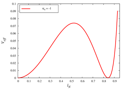
Figure 2: The $N=\infty$ effective potential for $\kappa_{4}=-1$, where the transition is strongly first order.

In an asymptotically free theory, the expectation value of a Polaykov loop approaches one at high temperature. It is perfectly conceivable that when a gauge theory deconfines, that it goes directly to a gluon plasma which is close to perturbative, even at temperatures just above $T_{d}$. (An example of this is Fig. (2) of Sec. III.4.) Indeed, if the deconfining phase transition is strongly first order, this is what one might naively expect. From lattice simulations, while the deconfining transition is of second order for two colors two_colors_A ; two_colors_B , it is of first order for three colors lattice_review ; three , and becomes more strongly first order as the number of colors increases. Results for four four_colors ; teper ; meyer , six, and eight colors teper ; meyer suggest that at large $N$, the latent heat is proportional to an obvious factor of $\sim N^{2}$, from the overall number of gluons in a deconfined phase, times a constant.

For three colors, the lattice measurements of the renormalized triplet loop are admittedly preliminary. With that caveat, the expectation value of the renormalized triplet loop is found to be near one, $\approx.9\pm 10\%$, for temperatures which are as low at $\approx 3T_{d}$. This agrees with resummations of perturbation theory, which work down from infinite temperature, but consistently fail at a temperature which is something like $\approx 3\rightarrow 5T_{d}$ resum .

Just above the transition, however, the renormalized triplet loop is far from one: it is only $\approx 0.4\pm 10\%$ at $T_{d}^{+}$. This suggests the following picture. For temperatures above $\approx 3T_{d}$, the deconfined plasma is, after resummation, nearly perturbative. For temperatures between $T_{d}$ and $\approx 3T_{d}$, however, the theory is in a phase which is deconfined but non-perturbative. The existence of such a non-perturbative (quark) gluon plasma may be indicated by the experimental data on heavy ion collisions at RHIC RHIC .

At large $N$, the deconfining transition has been studied using string and duality methods hagedorn ; previous ; aharony ; fss ; schnitzer ; aharony2 . At infinite $N$, by restricting the theory to live on a space-time where space is a very small sphere, it is possible to compute the Hagedorn temperature analytically hagedorn ; previous ; aharony ; fss ; schnitzer ; aharony2 . In this limit, Aharony et al. aharony catagorized the possible relationships between the deconfining, and the Hagedorn, temperatures.

In this paper we develop a general approach to the deconfining transition, based upon a matrix model of Polyakov loops. We begin in Sec. II with the most general effective Lagrangian, including all terms up to two spatial derivatives. At first sight, matrix models of loops appear to be an inelegant type of nonlinear sigma model banks_ukawa ; loop1 ; loop2a ; loop2b ; loop2c ; loop2d ; loop2e ; loop2f ; loop3 ; sannino ; ogilvie ; interface1 ; interface2 . This is not a matter of choice, but is dictated by the physics. For ordinary nonlinear sigma models, in the chiral limit there are no potential terms, only terms involving spatial derivatives. These can be studied in a mean field approximation, but this is only valid when the number of spacetime dimensions is large zinn ; drouffe_zuber ; largeN . In contrast, the effective action for loops starts with a potential, independent of spatial derivatives. Because of this, a systematic large $N$ expansion can be developed in any number of spacetime dimensions.

The large $N$ expansion of the loop potential is developed in Sec. III. We show how the Vandermonde determinant, which appears in the measure of the matrix model, gives a type of potential term brezin ; gross_witten ; aharony . also contributes a potential term. At infinite $N$, the vacua of the theory are then given by the stationary points of an effective potential, which is the sum of the loop, and what we call the Vandermonde, potentials.

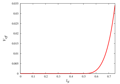
Figure 1: The $N=\infty$ effective potential at the Gross–Witten point. When $\ell_{N}<\frac{1}{2}$, the potential vanishes identically. In Figs. 1, 2, and 3, there is a discontinuity, of third order, at $\ell_{N}=\frac{1}{2}$, although it is only apparent here.

In the loop potential, the adjoint loop is a mass term, while loops in higher representations represent interaction terms. We show how the Gross–Witten model gross_witten ; jurk , which arose in a very different context, corresponds to a loop potential which is purely a mass term, with no higher terms. We term the point at which the deconfining transition occurs as the “Gross–Witten point” dhlop . At this point, the expectation value for the loop in the fundamental representation, $\ell$, jumps from $0$ to precisely $\frac{1}{2}$ dhlop ; aharony ; gross_witten ; kogut . The loop potential is most unusual, however: it vanishes identically for $\ell$ between $0$ and $\frac{1}{2}$, and is only nonzero when $\ell\geq\frac{1}{2}$ (see Fig. 1 below). This is only possible because of the contribution of the Vandermonde potential. This potential, which is not analytic in $\ell$ at $\ell=\frac{1}{2}$, produces a deconfining transition which is thermodynamically of first order dhlop ; aharony ; kogut . This flat potential also implies that at the transition point, masses vanish, asymmetrically, in both phases (these are the masses for the fundamental loop, along the direction of the condensate) dhlop . If a background field is added, at the Gross–Witten point the first order transition turns into one of third order, no matter how small the background field is green_karsch ; damgaard_patkos .

Aharony et al. analyzed the transition when quartic interactions are included aharony . They suggested that in the space of loop potentials, the Gross–Witten model represents a tri-critical point. We refine their analysis, and extend it to include arbitrary interactions of the fundamental loop. We discuss why the Gross–Witten point is more accurately described as an ultra-critical point, where all higher interactions vanish. Physically, this is defined as the unique point where the transition is of first order, and yet masses vanish; it only arises at infinite $N$.

We analyze the matrix integral by introducing a constraint field for the fundamental loop zinn . Various constraint fields can then be integrated out in different order. One order is equivalent to computing the Vandermonde potential by Legendre transformation aharony ; fss ; schnitzer ; aharony2 . We show that the other order is equivalent to what was called, previously, a mean field approximation kogut ; green_karsch ; damgaard_patkos ; dhlop . If the potential includes just the adjoint loop, we check that while these two methods give different effective potentials, that at any stationary point, both the expectation values of the loop, and masses, agree.

For three colors, the surprising aspect of the lattice data is that the value of the renormalized triplet loop at $T_{d}^{+}$, $\approx 0.4$, is close to $\frac{1}{2}$. Further, masses associated with the triplet loop — especially the string tension — decrease significantly near the transition three . This suggests that the transition for three colors is close to the Gross–Witten point at infinite $N$.

The lattice results provide further evidence for the utility of using a large $N$ expansion at $N=3$. The expectation values of renormalized sextet and octet loops, which are expected to be $\sim 1/N$ or smaller, never exceed $\approx 25\%$ at any temperature, and are usually much less dhlop .

In Sec. IV we study the loop potential for finite $N$. Following Damgaard et al. damgaard , we start by showing that when fluctuations in the matrix model are neglected, that the expectation value of any loop — including those which are $Z(N)\;$neutral — vanish in the confined phase. This is a striking difference between matrix models and more general $Z(N)\;$symmetric theories kiskis .

The matrix model is merely a two dimensional integral, which can be studied numerically. In Sec. IV we investigate theories close to the $N=3$ analogy of the Gross–Witten point, including cubic interactions. The matrix model gives the expectation values of loops in arbitrary representations. We also compute the mass of the loop, which is related to the (gauge invariant) Debye mass, as obtained from the two point function of Polyakov loops. We discuss how measurements of both the Debye mass, and the renormalized triplet loop, help probe the loop potential.

We also use the matrix model to compute difference loops dhlop for the sextet, octet, and decuplet loops. If only the loop potential is included, the difference loops from lattice simulations dhlop are not well reproduced. Presumably it is necessary to include fluctuations, due to kinetic terms, in the effective theory. Nevertheless, up to these small corrections, $\leq 20\%$ at all temperatures, it is clear that the deconfining transition for three colors is close to the Gross–Witten point at infinite $N$.

In the Conclusions, Sec. V, we discuss why lattice data four_colors ; teper ; meyer may indicate that the deconfining transitions for $N\geq 4$ are also near the Gross–Witten point. We suggest that one must be very close to the transition to see this, when the reduced temperature $|T-T_{d}|/T_{d}\sim 1/N^{2}$.

II Effective Models

II.1 Nonlinear Sigma Models

We begin by briefly reviewing effective theories for nonlinear sigma models zinn . For definiteness, consider the model appropriate to chiral symmetry breaking for $N_{f}$ flavors, with a global symmetry group of donoghue

$$G_{f}=SU_{L}(N_{f})\times SU_{R}(N_{f})\;,$$ (1)

and a field $U$, transforming as

$$U\rightarrow e^{2\pi ij/N_{f}}\;\Omega_{L}^{\dagger}\;U\;\Omega_{R}\;;$$ (2)

where $\Omega_{L,R}$ are $SU_{L,R}(N_{f})$ transformations. Because the left and right handed chiral rotations are distinct, in the chiral limit, terms such as the trace of $U$, ${\rm tr}\;U$, cannot arise. Thus in the chiral limit, there is no potential for $U$, and there are only derivative terms. These start at second order:

$${\cal L}=f^{2}_{\pi}\;{\rm tr}\;|\partial_{\mu}U|^{2}+\ldots\;;$$ (3)

subject to the constraint that $U$ is a unitary matrix,

$$U^{\dagger}U={\bf 1}_{N_{f}}\;.$$ (4)

The series then continues with terms of quartic order in derivatives donoghue .

After chiral symmetry breaking, what remains is a vector symmetry of $SU_{V}(N_{f})$, with $\Omega_{L}=\Omega_{R}=\Omega_{V}$. Then there is a potential for $U$ possible,

$${\cal V}=m^{2}_{\pi}\;{\rm tr}\;U\;+\ldots.$$ (5)

This potential is manifestly proportional to the pion mass squared, since it must vanish in the chiral limit. Near the chiral limit, the kinetic terms in (3) dominate over the potential term in (5) if the volume of space (or space-time) is large. If the volume is small, however, the potential term can dominate, as the modes with nonzero momentum are frozen out epsilon .

Other sigma models are constructed by allowing the transformations $\Omega_{L}$ and $\Omega_{R}$ to be equal. For example, take $U$ to be a $SU(2N_{f})$ matrix, and impose a further constraint, such as that the trace of $U$ vanishes, ${\rm tr}\;\,U=0$. In this case, the symmetry is that of a symmetric space, $G_{f}=SU(2N_{f})/S(U(N_{f})\times U(N_{f}))$ zinn ; symmetric . Because the trace of $U$ is constrained to be a fixed number, there is no potential possible, and the action is given entirely by kinetic terms, as in (3). If the trace is constrained to be some other value, then the symmetry group changes, but there is still no potential possible.

These nonlinear sigma models are renormalizable in an expansion about two space-time dimensions. There is a phase with broken symmetry above two dimensions, where the expectation value of $U$ is nonzero. This expectation value is generally not proportional to the unit matrix, and there are Goldstone bosons in the broken phase. In the chiral limit, as there is no potential for $U$, it is not easy studying the possible patterns of symmetry breaking directly in the nonlinear form of the model (linear models are usually more useful). Symmetry breaking can be studied using mean field theory zinn ; drouffe_zuber . To do so, the continuum form of the theory is replaced by a lattice form, with matrices $U$ on each site $i$. In that case, the next to nearest neighbor interaction at a site $i$, for unit lattice vector $\hat{n}$, becomes, in mean field approximation,

$${\rm tr}\;\left(U_{i}U_{i+\hat{n}}\right)\rightarrow{\rm tr}\;\left(U_{i}\;\langle U\rangle\right)\;.$$ (6)

In this case, mean field theory is only applicable when the number of nearest neighbors, or space-time dimensions, is very large zinn ; drouffe_zuber .

II.2 Polyakov Loops: Preliminaries

We discuss the deconfining transition at a nonzero temperature $T$, for a space of infinite volume. The analysis is more general, though, and can be easily extended to the case in which space is of finite extent, etc.

The thermal Wilson line is

$${\bf L}_{\cal R}(\vec{x})={\cal P}\;\exp\left(ig\int^{1/T}_{0}A_{0}^{a}(\vec{x},\tau)\;{\bf t}^{a}_{\cal R}\;d\tau\right)\;.$$ (7)

We follow our previous notations and conventions dhlop . We define the thermal Wilson line at a point $\vec{x}$ in space, letting it run all of the way around in imaginary time, from $0$ to $\tau=1/T$. Otherwise, ${\cal P}$ denotes path ordering, $g$ is the gauge coupling constant, and $A_{0}^{a}$ the vector potential in the time direction. The ${\bf t}^{a}_{\cal R}$ are the generators of $SU(N)$ in a representation ${\cal R}$, which is taken to be irreducible.

The Wilson line transforms homogeneously under local gauge transformations,

$${\bf L}_{\cal R}(\vec{x})\rightarrow\Omega_{\cal R}^{\dagger}(\vec{x},1/T)\;{\bf L}_{\cal R}(\vec{x})\;\Omega_{\cal R}(\vec{x},0)\;.$$ (8)

For gauge transformations which are periodic in imaginary time, we form a gauge invariant quantity, the Polyakov loop in ${\cal R}$, by taking the trace,

$$\ell_{\cal R}=\frac{1}{d_{\cal R}}\;{\rm tr}\;\,{\bf L}_{\cal R}\;.$$ (9)

We define the Polyakov loop as the normalized trace of ${\bf L}_{\cal R}$, with $d_{\cal R}$ equal to the dimension of ${\cal R}$. The advantage of this is that in an asymptotically free theory, all Polyakov loops are of unit magnitude in the limit of infinitely high temperature. We denote representations by their dimensionality, with two exceptions, which differ from previous use dhlop . The Wilson line in the fundamental representation is ${\bf L}$, with the fundamental loop

$$\ell_{N}=\frac{1}{N}\;{\rm tr}\;\,{\bf L}\;.$$ (10)

The adjoint loop is denoted

$$\ell_{ad}=\frac{1}{N^{2}-1}\left(\,|{\rm tr}\;{\bf L}|^{2}-1\right)\;.$$ (11)

Besides local gauge transformations, which are strictly periodic in time, in a pure gauge theory there are also global gauge transformations, which are only periodic up to an element of the center of the gauge group. For an $SU(N)$ gauge group, the center is $Z(N)\;$. In the fundamental representation, the simplest global $Z(N)\;$transformation is

$$\Omega(\vec{x},1/T)=e^{2\pi i/N}\;\Omega(\vec{x},0)\;.$$ (12)

Defining the charge of the fundamental representation to be one, the charge of an arbitrary representation, $e_{\cal R}$, follows from its transformation under (12),

$$\ell_{\cal R}\rightarrow e^{2\pi ie_{\cal R}/N}\ell_{\cal R}\;.$$ (13)

As a cyclic group, the charge $e_{\cal R}$ is only defined modulo $N$. A special set of representations are those with zero $Z(N)\;$charge, which we denote as ${\cal R}_{0}$. The simplest example is the adjoint representation.

Below the deconfining transition temperature $T_{d}$, the expectation values of all loops with nonzero $Z(N)\;$charge vanish,

$$\langle\ell_{\cal R}\rangle=0\;\;\;,\;\;\;T\leq T_{d}\;\;\;,\;\;\;{\cal R}\neq{\cal R}_{0}\;,$$ (14)

and the theory is in a $Z(N)\;$symmetric phase.

The global $Z(N)\;$symmetry is broken in the deconfined phase, as loops in all representations condense,

$$\langle\ell_{\cal R}\rangle\neq 0\;\;\;,\;\;\;T\geq T_{d}\;\;\;,\;\;\;\forall\;{\cal R}\;.$$ (15)

In the limit of large $N$, factorization dhlop ; drouffe_zuber ; largeN implies that all expectation values are powers of that for the fundamental, and anti-fundamental, loops:

$$\langle\ell_{R}\rangle=\langle\ell_{N}\,\rangle^{p_{+}}\;\langle\ell_{N}^{*}\rangle^{p_{-}}\;\;\;,\;\;\;N=\infty\;.$$ (16)

The integers $p_{+}$ and $p_{-}$ are defined in dhlop . For the adjoint, for example, $p_{+}=p_{-}=1$; in general, the $Z(N)\;$charge $e_{\cal R}=p_{+}-p_{-}$. Factorization is exact only at infinite $N$, but holds for all temperatures. Corrections to factorization are of order $\sim 1/N$ at large $N$; for the adjoint, they are $\sim 1/N^{2}$ dhlop .

In general, loops with zero $Z(N)\;$charge, such as the adjoint, can have nonzero expectation values at all temperatures, including in the confined phase. At infinite $N$, factorization implies that they vanish below $T_{d}$, because the expectation value of the fundamental loop does. An important question to which we shall return is the extent to which $Z(N)\;$neutral loops condense in the confined phase.

II.3 Matrix Models of Polyakov Loops

In the same spirit as familiar for effective models of chiral symmetry breaking donoghue ; epsilon , discussed in Sec. II.1, we construct an effective theory for deconfinement, applicable over distances greater than the inverse temperature. Thus fields depend only upon the spatial coordinates, $\vec{x}$. We take as the basic field the Wilson line, ${\bf L}(\vec{x})$; as that is a gauge covariant field, we need also include the spatial components of the vector potential, $A_{i}(\vec{x})$.

We are then led to construct the most general action consonant with the relevant symmetries, which are those of global $Z(N)\;$, and local $SU(N)$, transformations. We will allow the vacuum to spontaneously break the $Z(N)\;$symmetry, but do not allow $SU(N)$ to break. (It would be interesting to extend the following analysis to include a Higgs phase, as is appropriate for symmetry restoration in the electroweak interactions.)

We start with potential terms, independent of any derivatives in space-time. Because of the left-right symmetry, for sigma models there is no potential in the chiral limit. In constrast, loop models always have a potential. To be invariant under $SU(N)$ transformations, terms in the potential must be a sum of loops; to be invariant under $Z(N)\;$, these must be $Z(N)\;$neutral:

$${\cal V}({\bf L})=-m^{2}\,\ell_{ad}+\sum_{{\cal S}\epsilon{\cal R}_{0}}\;\kappa_{\cal S}\;{\rm Re}\;\ell_{\cal S}\;;$$ (17)

Loops can be complex valued when $N\geq 3$, so in the potential we take the real part of each loop.

By using group theory, this potential can be rewritten in many different ways. As higher powers of any loop can always be reexpressed as a linear sum over loops in other representations, this potential is the most general form possible.

In ${\cal V}({\bf L})$, the adjoint loop looks like a mass term for the fundamental loop, while loops in higher representations look like interactions of the fundamental loop (plus new terms, such as ${\rm tr}\;{\bf L}^{2}/N$, etc.). The loop potential differs from that of ordinary scalar fields, though. In the potential of a scalar field, the coupling constant for the highest power of the field must be positive in order for a ground state to exist. This isn’t true for the loop potential, as each loop is bounded by one: there is no constraint whatsoever on the signs of the mass squared, nor on any of the coupling constants. For example, we choose the sign of the adjoint loop to have a negative sign (so that $m^{2}\sim T-T_{d}$, as for ordinary spin systems). Then $m^{2}\rightarrow-\infty$ drives one to the confined phase, while $m^{2}\rightarrow+\infty$ drives one into the deconfined phase. Further, it is consistent to have just a mass term, with no other terms in the potential, setting all $\kappa_{\cal S}=0$. Thus while the adjoint loop looks like a mass term for the fundamental loop, because the basic variable is ${\bf L}$, and not $\ell_{N}$, the theory is still nontrivial with no “interactions”, $\kappa_{\cal S}=0$.

At each point in space, the Wilson line can be diagonalized by a local gauge transformation, and so depends upon $N-1$ eigenvalues. Thus instead of ${\bf L}$, it is also possible to chose a set of $N-1$ loops, and rewrite the loop potential in terms of these. We find this of use in Sec. IV, (70).

The loop potential can be computed analytically in two limits: when the temperature is very high interface1 ; interface2 , and when space is a small sphere hagedorn ; previous ; aharony ; fss ; schnitzer ; aharony2 . For both cases there is a large mass scale, either the temperature, or the inverse radius of the sphere, so that the effective gauge coupling is small by asymptotic freedom. In perturbation theory, the loop potential is computed from the one loop determinant in the presence of a background gauge potential $A_{0}\sim\log{{\bf L}}$ hagedorn ; previous ; aharony ; fss ; schnitzer ; aharony2 ; interface1 ; interface2 . At very high temperature (and infinite spatial volume), while the result can be written in terms of an infinite polynomial of (traces of) powers of ${\bf L}$, as in (17), the sum can be explicitly performed. The result is just a a simple quartic potential of $A_{0}$ interface1 .

In a perturbative regime, it is natural that the loop potential is more transparent in terms of elements of the Lie algebra, the $A_{0}$, instead of elements of the Lie group, the ${\bf L}$. This suggests that an effective theory of loops is not especially convenient when the theory is essentially perturbative. For $SU(3)$, resummations of perturbation theory suggest that the perturbative regime appears for $T\approx 3T_{d}$ resum . Thus for $SU(3)$, loops are only useful for temperatures below $\approx 3T_{d}$.

The loop potential can also be computed on a small sphere previous ; aharony ; fss ; schnitzer ; aharony2 . There are now two scales in the problem — the radius of the system, and the temperature — so the result is much more complicated than for infinite volume. The result is a sum like that of (17).

Kinetic terms, involving two derivatives, are constructed similarly. While sigma models only have one term with two derivatives, (3), due to the change in symmetry, loop models have an abundance. One class of terms involves covariant derivatives of the Wilson line:

$${\cal K}_{1}({\bf L})=\frac{1}{\widetilde{g}^{2}}\;{\rm tr}\;|D_{i}{\bf L}|^{2}\left(1+\sum_{{\cal S}\epsilon{\cal R}_{0}}\;\lambda_{\cal S}\;\;{\rm Re}\,\ell_{\cal S}\right)$$ (18)

The first term is a sort of “electric loop”: it is the original electric field of the gauge theory, rewritten in terms of loops. At tree level, the coupling constant $\widetilde{g}$ equals the gauge coupling $g$, but in general, it is an independent coupling constant of the effective theory. Besides the electric loop, there is an infinite series of terms involving loops in $Z(N)\;$neutral representations. The couplings of magnetic fields is similar to (18): there is an infinite series of $Z(N)\;$neutral loops which couple to the (trace of the) magnetic field squared.

There are also derivative terms for the loops themselves:

$${\cal K}_{2}({\bf L})=\frac{1}{\widetilde{g}^{4}}\;\sum_{{\cal S},{\cal S}^{\prime},{\cal S}^{\prime\prime}\epsilon{\cal R}}\;\zeta_{{\cal S},{\cal S}^{\prime},{\cal S}^{\prime\prime}}\;{\rm Re}\;\left(\partial_{i}\ell_{\cal S}\right)\left(\partial_{i}\ell_{{\cal S}^{\prime}}\right)\;\ell_{{\cal S}^{\prime\prime}}\;,$$ (19)

where the representations are constrained so that the total $Z(N)\;$charge of each term vanishes, $e_{{\cal S}}+e_{{\cal S}^{\prime}}+e_{{\cal S}^{\prime\prime}}=0$, modulo $N$.

Lastly, there are terms involving two derivatives of ${\bf L}$, coupled to a field with $Z(N)\;$charge minus two:

$${\cal K}_{3}({\bf L})=\frac{1}{\widetilde{g}^{2}}\;{\rm tr}\;\;{\rm Re}\;(D_{i}{\bf L})^{2}\;\sum_{{\cal S}\epsilon{\cal R}}\;\widetilde{\zeta}_{\cal S}\;\ell_{\cal S}\;\;\;,\;\;\;e_{\cal S}=-2\;.$$ (20)

For three colors, this series starts with the triplet loop.

In the deconfined phase, the free energy is of order $\sim N^{2}$. Since all loops are of order one at large $N$, in the action we always assume that the potential ${\cal V}$ is multiplied by an overall factor of $\sim N^{2}$ at large $N$. The mass $m^{2}$ is then naturally of order one at large $N$; how the coupling constants $\kappa_{\cal S}$ scale with $N$ is discussed in Sec. III.5. For the kinetic terms, to contribute $\sim N^{2}$, the coupling $\widetilde{g}$ should scale like the gauge coupling, with $g^{2}N$ and $\widetilde{g}^{2}N$ fixed at large $N$; then the couplings $\zeta_{{\cal S},{\cal S}^{\prime},{\cal S}^{\prime\prime}}$ and $\widetilde{\zeta}_{\cal S}$ are both $\sim 1$.

The renormalization of the loop potential was discussed in dhlop . The Wilson line in a given, irreducible representation undergoes mass renormalization, $m^{div}_{\cal R}$; on a lattice, this is a power series in the coupling constant times the lattice spacing, $1/a$. For a Wilson line at a temperature $T$, the renormalization constant, ${\cal Z}_{\cal R}$, and the renormalized loop, $\widetilde{\ell}_{\cal R}$, are given by

$$\widetilde{\ell}_{\cal R}=\ell_{\cal R}/{\cal Z}_{\cal R}\;\;\;,\;\;\ {\cal Z}_{\cal R}=\exp(-m^{div}_{\cal R}/T)\;.$$ (21)

Loops in irreducible representations do not mix under renormalization.

The renormalization constants for the kinetic terms are similar, but more involved, than those for the potential. All kinetic terms undergo mass renormalization, with renormalization constants which are the exponential of a divergent mass times the length of the loop. For loops without cusps, there is no condition to fix the value of these renormalization constants at some scale, while loops with cusps do require such a condition dhlop ; cusp ; difference . For kinetic terms, additional renormalization constants, and conditions to fix their value at some scale, may be required. For example, each term in (18) experiences mass renormalization. In addition, since the term $\sim 1/\widetilde{g}^{2}$ arises from the electric field in the bare action, at least in four spacetime dimensions, it will require an additional renormalization constant related to coupling constant renormalization.

We have written down all possible terms involving two derivatives, but this classification may well be overly complete. In particular, renormalization will greatly restrict the possible terms. The entire list is relevant in two spatial dimensions; the associated $\beta$-functions can be computed in the ultraviolet limit beta . In three spatial dimensions, a scalar field has dimensions of the square root of mass, and most of the above terms are non-renormalizable, and so can be ignored.

Terms which arise from the coupling to fields which are not $Z(N)\;$invariant, such as quark fields, can also be included. The simplest possible coupling involves the trace of the chiral field:

$$m^{2}_{\pi}\;{\rm tr}\;U\;{\rm Re}\;\ell_{N}\;.$$ (22)

This, however, is chirally suppressed, proportional to $m_{\pi}^{2}$. There are couplings which are not chirally suppressed, but these necessarily involve derivatives of the chiral field; these start as

$${\rm tr}\;|\partial_{\mu}U|^{2}\;{\rm Re}\;\ell_{N}\;.$$ (23)

We do not know if this chiral suppression significantly affects the breaking of $Z(N)\;$symmetry; in mean field theory, this can be analyzed by using a nonlinear sigma model for the chiral fields mean . For an analysis of $Z(N)\;$breaking terms in terms of linear sigma models, see Moscy, Sannino, and Tuominen sannino .

III Infinite N

III.1 Gross–Witten Point

The effective action for loops is much more involved than for sigma models. Because loops have a potential, however, we can systematically perform a large $N$ expansion by minimizing an effective potential. Corrections in $1/N$ arise from fluctuations, which arise when spatial derivatives are included. In the rest of the paper, we ignore fluctuations, and the kinetic terms of Sec. II.3, to concentrate on what is a matrix-valued mean field theory. Sec. III treats this matrix model at infinite $N$; Sec. IV, finite $N$. Even at infinite $N$, we stress that because we cannot compute the loop potential from first principles, all we are doing is characterizing all possible transitions in terms of couplings in the loop potential, the $\kappa_{\cal S}$ of (17).

If fluctuations are neglected, we can assume that the Wilson line is the same at each point in space, ${\bf L}(\vec{x})={\bf L}$. Thus the functional integral reduces to a single integral,

$${\cal Z}=\int d{\bf L}\;\exp\left(-N^{2}{\cal V}({\bf L})\right)\;.$$ (24)

At large $N$, factorization implies that for arbitrary representations, normalized loops are just products of the fundamental, and anti-fundamental, loop dhlop . Then the loop potential reduces simply to a power series in $|\ell_{N}|^{2}$,

$${\cal V}({\bf L})=-m^{2}|\ell_{N}|^{2}+\kappa_{4}\left(|\ell_{N}|^{2}\right)^{2}+\kappa_{6}\left(|\ell_{N}|^{2}\right)^{3}+\ldots\;.$$ (25)

We have relabeled the couplings $\kappa_{\cal S}$ in (17) as $\kappa_{2n}$, where the subscript now denotes the power of $\ell_{N}$. The $U(1)$ symmetry is broken to $Z(N)\;$by a term $\sim\kappa_{N}\,{\rm Re}\,(\ell_{N})^{N}$, but this is negligible at large $N$.

As the potential is multiplied by an overall factor of $\sim N^{2}$, and the loops are normalized to be of order one, the natural guess is also to take the couplings $\kappa_{\cal S}$ of order one at large $N$. As we discuss in Sec. III.5, this choice of couplings is far from innocuous. The advantage is that this assumption vastly simplifies the analysis, and allows us to gain insight which is otherwise obscured by technical complications aharony . Further, as far as the bulk thermodynamics is concerned, the only novel behavior emerges in this regime; otherwise, the deconfining transition is rather ordinary.

To find the stationary points of the functional integral, we introduce a delta-function into the integral zinn as

$${\cal Z}=\int d{\bf L}\;\int d\lambda\;\;\delta(\lambda-\ell_{N})\;\exp\left(-N^{2}{\cal V}(\lambda)\right)\;.$$ (26)

Here $\lambda$ is a (complex) number, equal to the value of $\ell_{N}={\rm tr}\;{\bf L}/N$ for a given matrix ${\bf L}$. As such, in the action we can replace ${\cal V}(\ell_{N})$ by ${\cal V}(\lambda)$. The constraint is then exponentiated by introducing a field $\overline{\omega}$,

$${\cal Z}=\int d\lambda\int d\overline{\omega}\int d{\bf L}\;\exp\left(-N^{2}{\cal V}_{cons.}\right)\;,$$

$${\cal V}_{cons.}={\cal V}(\lambda)+i\overline{\omega}(\lambda-\ell_{N})\;.$$ (27)

In this expression, both $\lambda$ and $\overline{\omega}$ are complex numbers, not matrices, or traces thereof. Usually, $i\overline{\omega}$ is real at a stationary point, and so we define $\omega=i\overline{\omega}$.

The full integral is over $\lambda$, $\overline{\omega}$, and ${\bf L}$. We break off the integral over ${\bf L}$, and define that piece as

$${\cal Z}_{GW}(\omega)=\int d{\bf L}\;\exp\left(N^{2}\,\omega\;{\rm Re}\,\ell_{N}\right)\;.$$ (28)

By an overall $Z(N)\;$rotation, we can choose any condensate for $\ell_{N}$ to be real and positive. Both $\lambda$ and $\omega$ are complex fields, but to look for a real stationary point in $\ell_{N}$, we need only consider the real parts.

The integral ${\cal Z}_{GW}$ was done by Brezin et al. brezin , Gross and Witten gross_witten , and Aharony et al. aharony . For the unitary matrix ${\bf L}$, all that matters are the eigenvalues of ${\bf L}$, ${\bf L}_{i,j}=\delta_{ij}\exp(i\alpha_{i})$. In the limit of infinite $N$, the number of eigenvalues is infinite, and it is convenient to introduce the density of eigenvalues, $\rho(\alpha)$. The solution for this density is:

$$\rho(\alpha)=\frac{1}{2\pi}\left(1+\omega\,\cos\alpha\right)\;\;\;,\;\;\;\omega\leq 1\;;$$ (29)

$$\rho(\alpha)=\frac{1}{\pi}\;\cos\frac{\alpha}{2}\left(1-\omega\;\sin^{2}\frac{\alpha}{2}\right)^{1/2}\;\;\;,\;\;\;\omega\geq 1\;$$ (30)

where the latter only holds for $\omega\;\sin^{2}(\alpha/2)<1$.

We now make the following observation. The value of the condensate is

$$\ell_{0}=\int^{\pi}_{-\pi}d\alpha\;\rho(\alpha)\cos\alpha\;.$$ (31)

With these expressions for the eigenvalue density, it is not difficult to show that

$$\ell_{0}(\omega)=\frac{\omega}{2}\;\;\;,\;\;\;\omega\leq 1\;;$$ (32)

and

$$\ell_{0}(\omega)=1-\frac{1}{2\omega}\;\;\;,\;\;\;\omega\geq 1\;;$$ (33)

To implement these relations between the expectation value and $\omega$, we introduce yet another constraint field, $\ell$, along with a function, ${\cal V}_{V\!dm}(\ell)$, as follows:

$${\cal Z}_{GW}(\omega)=\int d\ell\;\exp\left(N^{2}\left(\omega\ell-{\cal V}_{V\!dm}(\ell)\right)\right)\;.$$ (34)

$\ell$ is just a complex number, so the stationary point of this integral occurs when

$$\omega=\left.\frac{\partial{\cal V}_{V\!dm}}{\partial\ell}\right|_{\ell=\ell_{0}}\;.$$ (35)

It is then trivial to see that if we choose

$${\cal V}_{V\!dm}(\ell)=+\;\ell^{2}\;\;\;,\;\;\;\ell\leq\frac{1}{2}\;;$$ (36)

$${\cal V}_{V\!dm}(\ell)=-\frac{1}{2}\log\left(2\left(1-\ell\right)\right)+\frac{1}{4}\;\;\;,\;\;\;\ell\geq\frac{1}{2}\;.$$ (37)

then (35) gives the desired relations, (32) and (33). One can also check that (34) gives the correct result for ${\cal Z}_{GW}(\omega)$ gross_witten .

Using this form of ${\cal V}_{V\!dm}$ in (34), and replacing $\omega=i\overline{\omega}$, the original partition function becomes

$${\cal Z}=\int d\lambda\int d\overline{\omega}\int d\ell\;\exp\left(-N^{2}\,{\cal V}^{\prime}\;\right)\;,$$

$${\cal V}^{\prime}={\cal V}(\lambda)+i\overline{\omega}(\lambda-\ell)+{\cal V}_{V\!dm}(\ell)\;.$$ (38)

Doing the integral over $\overline{\omega}$ fixes $\lambda=\ell$, and leaves

$${\cal Z}=\int d\ell\;\exp\left(-N^{2}\,{\cal V}_{e\!f\!f}(\ell)\right)\;.$$ (39)

The effective potential,

$${\cal V}_{e\!f\!f}(\ell)={\cal V}(\ell)+{\cal V}_{V\!dm}(\ell)\;,$$ (40)

is the sum of the loop potential, which we started with, and ${\cal V}_{V\!dm}$. Unlike the original integral over the matrix ${\bf L}$, (39) is just an integral over a single degree of freedom, $\ell$. Since the effective potential is multiplied by an overall factor of $N^{2}$, at large $N$ the true vacua of the theory are the stationary points of ${\cal V}_{e\!f\!f}(\ell)$.

When we introduce ${\cal V}_{V\!dm}(\ell)$ in (34), mathematically this is just the Legendre transformation of ${\cal Z}_{GW}$ zinn , treating $\omega$ as an external source for $\ell$. This is nontrivial only because in ${\cal Z}_{GW}$, the measure for the matrix ${\bf L}$ includes the Vandermonde determinant. For this reason, we refer to ${\cal V}_{V\!dm}(\ell)$ as the “Vandermonde potential”.

Note that the Vandermonde potential is just the Legendre transformation of ${\cal Z}_{GW}$, and not of the full integral. One could compute the Legendre transformation of $\cal Z$, but of necessity, this would also include the loop potential. When the transition occurs, however, the effective potential has degenerate vacua, and ${\cal V}_{e\!f\!f}(\ell)$ is not a monotonic function of $\ell$. This leads to well known ambiguities in the Legendre transformation zinn . In contrast, the Vandermonde potential is a monotonically increasing function of $\ell$, and there is never any ambiguity in its Legendre transformation. This remains true at finite $N$, Sec. IV.2.

The Vandermonde potential vanishes at $\ell=0$, and diverges, logarithmically, as $\ell\rightarrow 1$. At $\ell=\frac{1}{2}$, the value of ${\cal V}_{V\!dm}(\ell)$, and its first and second derivatives, are continuous. The third derivative is not, since it vanishes for $\ell<\frac{1}{2}$, and is nonzero for $\ell>\frac{1}{2}$.

For a lattice theory, $\omega$ is an inverse coupling constant. With a Wilson action, there implies a transition, of third order, in $\omega$. This disappears if the lattice action is other than Wilson, however. In contrast, the Vandermonde potential always has a discontinuity, of third order, at $\ell=\frac{1}{2}$. Because it is a transition of such high order, it may not affect the bulk thermodynamics significantly, but it is always there.

The form of the Vandermonde potential is of interest. While it is nonpolynomial when $\ell\geq\frac{1}{2}$, $\sim\log(1-\ell)$, this is just eigenvalue repulsion from the Vandermonde determinant. This is why there are no constraints on the signs of the couplings in the loop potential: eigenvalue repulsion never lets the value of $\ell$ exceed one.

About the origin, the Vandermonde potential is just a mass term, but in fact that is the most interesting thing about it. All terms of order $\sim\ell^{4}$, $\sim\ell^{6}$, and so on, conspire to cancel kogut . In a miracle of group theory, the leading correction is of very high order, starting out as $\sim\ell^{N}$.

Given the effective potential, it is then immediate to read off the phase diagram of the theory. For a given value of $m^{2}$ and the coupling constants, one just varies with respect to $\ell$, as one would for any other potential.

For a given value of $m^{2}$, we denote the stable minimum as $\ell_{0}$. The confined vacuum has $\ell_{0}=0$: if the confined vacuum is a stable minimum of the loop potential, then because of the simple form of the Vandermonde potential, it remains so for the effective potential, with ${\cal V}_{e\!f\!f}(0)=0$.

A vacuum in the deconfined phase satisfies

$$\left.\frac{\partial{\cal V}_{e\!f\!f}(\ell)}{\partial\ell}\right|_{\ell=\ell_{0}}=0\;,$$ (41)

with $\ell_{0}\neq 0$. The transition occurs when the deconfined phase is degenerate with the confined phase,

$${\cal V}_{e\!f\!f}(\ell_{0}^{+})=0\;;$$ (42)

$\ell_{0}^{+}$ denotes the value of the order parameter at the transition, approaching it in the deconfined phase.

The simplest possible example is to ignore all couplings in the loop potential, and simply take

$${\cal V}(\ell)=-m^{2}\;\ell^{2}\;.$$ (43)

About the origin, the potential is

$${\cal V}_{e\!f\!f}(\ell)=(-m^{2}+1)\;\ell^{2}\;\;\;,\;\;\;\ell\leq\frac{1}{2}\;.$$ (44)

and

$${\cal V}_{e\!f\!f}(\ell)=-m^{2}\;\ell^{2}-\frac{1}{2}\log\left(2\left(1-\ell\right)\right)+\frac{1}{4}\;\;\;,\;\;\;\ell\geq\frac{1}{2}\;.$$ (45)

In the confined phase the potential is just a mass term. Its sign shows that a transition occurs at $m^{2}=1$, between a confined phase, for $m^{2}<1$, and a deconfined phase, for $m^{2}>1$. In the deconfined phase, the condensate is the solution of

$$-2m^{2}\ell_{0}+\frac{1}{2(1-\ell_{0})}=0\;,$$ (46)

which is

$$\ell_{0}=\frac{1}{2}\left(1+\sqrt{1-\frac{1}{m^{2}}}\right)\;.$$ (47)

(There is another solution to the quadratic equation, but it has $\ell_{0}<\frac{1}{2}$, and so doesn’t matter.)

The effective potential at the transition, $m^{2}=1$, is shown in Fig. 1. We call this the “Gross–Witten point”. At the transition, the potential vanishes for $\ell$ between $0$ and $\ell_{0}^{+}=\frac{1}{2}$; it then increases for $\ell>\frac{1}{2}$. Away from the Gross–Witten point, the potential is rather ordinary. In the confined phase, it is monotonically increasing from $\ell=0$. In the deconfined phase, the global minimum has $\ell_{0}\neq 0$. (For $m^{2}>1$, $\ell=0$ is actually metastable, since although there is no barrier, the first derivative of ${\cal V}_{e\!f\!f}$ vanishes at $\ell=0$.) As $m^{2}$ increases in value from one, the minimum moves from $\frac{1}{2}$ to larger values, approaching one only asymptotically in the limit of $m^{2}\rightarrow\infty$. For any value of $m^{2}$, either positive or negative, there is only one stable minimum.

We can also compute the effective mass squared. With this method, it is simply the second derivative of the potential about the minimum,

$$m^{2}_{eff}=\left.\frac{\partial^{2}{\cal V}_{e\!f\!f}(\ell)}{\partial\ell^{2}}\right|_{\ell=\ell_{0}}.$$ (48)

In the confined phase,

$$m^{2}_{eff}=2(1-m^{2})\;\;\;,\;\;\;m^{2}\leq 1\;.$$ (49)

In the deconfined phase, using (46) we can write

$$m^{2}_{eff}=\frac{2\ell_{0}-1}{2\ell_{0}(1-\ell_{0})^{2}}\;\;\;,\;\;\;\ell_{0}\geq\frac{1}{2}\;.$$ (50)

About the transition,

$$m^{2}_{eff}\approx 4\sqrt{m^{2}-1}+\ldots\;\;\;,\;\;\;m^{2}\rightarrow 1^{+}\;.$$ (51)

This difference occurs because at the Gross–Witten point, the new minimum is right at the point where there is a discontinuity of third order. Both masses vanish at the transition, but do so asymetrically, with different powers of $|m^{2}-1|$.

To go further, we need to make some assumption about the relationship between the coefficients of the loop potential and the temperature. We assume a mean field relation between the adjoint mass and the temperature $m^{2}-1\sim T-T_{d}$, neglecting the variation of the coupling constants with temperature. As the transition is approached in the confined phase, $m^{2}_{eff}\sim T_{d}-T$ as $T\rightarrow T_{d}^{-}$, while in the deconfined phase, $m^{2}_{eff}\sim(T-T_{d})^{1/2}$ for $T\rightarrow T_{d}^{+}$ dhlop .

At the transition, the potential vanishes at both degenerate minima, ${\cal V}_{e\!f\!f}(0)={\cal V}_{e\!f\!f}(\ell_{0}^{+})=0$. The derivative with respect to $m^{2}$ is discontinuous, though, vanishing in the confined phase, but nonzero in the deconfined phase,

$$\left.\frac{\partial{\cal V}_{e\!f\!f}(\ell)}{\partial T}\right|_{T\rightarrow T_{d}^{+}}\sim\left.\frac{\partial{\cal V}_{e\!f\!f}(\ell)}{\partial m^{2}}\right|_{m^{2}\rightarrow 1^{+}}=\frac{1}{4}\;,$$ (52)

which shows that the latent heat is nonzero, arising entirely from the deconfined phase. The transition is “critical” first order dhlop : although masses vanish, the order parameter jumps.

Our discussion of the Vandermonde potential follows that of Aharony et al. aharony . They argue that if the loop potential contains operators such as ${\rm tr}\;{\bf L}^{2}/N$, ${\cal V}_{e\!f\!f}(\ell)$ can only be plotted for $\ell<\frac{1}{2}$. For potentials which are simply powers of the fundamental loop, however, we assert that the effective potential is meaningful, and most illuminating to plot, over its entire range, for $\ell:0\rightarrow 1$. In Sec. III.5 we outline how to compute the effective potential for arbitrary loop potentials.

III.2 Nonzero Background Field

Minimizing the effective potential is an elementary exercise in algebra. We begin with a background $Z(N)\;$field, taking the loop potential to be

$${\cal V}({\bf L})=-h\;{\rm Re}\,\ell_{N}-m^{2}\,|\ell_{N}|^{2}\;.$$ (53)

In this case, there is a nontrivial minimum of the effective potential for any nonzero value of $h$. When $\ell_{0}\leq\frac{1}{2}$, it is

$$\ell_{0}=\frac{h}{2(1-m^{2})}\;,$$ (54)

while for $\ell_{0}\geq\frac{1}{2}$,

$$\ell_{0}=\frac{1}{2}\left(1-\frac{h}{2m^{2}}+\sqrt{\left(1+\frac{h}{2m^{2}}\right)^{2}-\frac{1}{m^{2}}}\right)\;.$$ (55)

Consider the case where $h$ is infinitesimally small. If $m^{2}-1$ is not $\sim h$, we can expand in $h$: $\ell_{0}(h)\approx h/2$ when $\ell_{0}<\frac{1}{2}-O(h)$, while

$$\ell_{0}(h)\approx\ell_{0}(h=0)+\left(-1+\frac{1}{\sqrt{1-m^{-2}}}\right)\frac{h}{4m^{2}}+\ldots$$ (56)

for $\ell_{0}>\frac{1}{2}+O(h)$. Thus away from $\ell_{0}\sim\frac{1}{2}$, on both sides of the transition the shift in $\ell_{0}$ is small, of order $\sim h$ (see e.g. Fig. 2 in loop2e ). When $m^{2}-1\sim h$, though, the solution differs by a large amount from that for $h=0$. There is a third order transition when $\ell_{0}$ equals $\frac{1}{2}$. The value at which this happens is easiest to read off from (54). This occurs for $m^{2}=1-h$, at which point the effective mass squared $m^{2}_{eff}=2h$.

For an ordinary first order transition, as the value of a background field increases from zero, there is still a nonzero jump in the order parameter. The jump only disappears for some nonzero value of the background field, which is a critical endpoint. For larger values, there is no jump in the order parameter, and masses are always nonzero. For the loop potential of (53), however, any nonzero background field, no matter how small, washes out the first order transition. For any $h\neq 0$, there is still a transition of third order, at which the masses are nonzero.

These results give an elementary interpretation of the calculations of Schnitzer schnitzer . He computed the partition function for quarks in the fundamental representation coupled to $SU(\infty)$ gauge fields, taking space to be a very small sphere. Fields in the fundamental representation break the $Z(N)\;$symmetry, and act like a background field $h\sim N_{f}/N$, where $N_{f}$ is the number of flavors. When $m^{2}<1-h$, by (54) $\ell_{0}\sim h\sim N_{f}/N$; substituting this back into (53), the potential, and so the free energy, is of order ${\cal V}_{e\!f\!f}(\ell_{0})\sim h^{2}\sim(N_{f}/N)^{2}$. The first order transition disappears for any $h\neq 0$ green_karsch , leaving just a transition, of third order, when $\ell_{0}$ passes through $\frac{1}{2}$ damgaard_patkos .

III.3 Mean Field Approximation

The analysis in Secs. III.1 and III.2 is most transparent for understanding the physics. Following Kogut, Snow, and Stone dhlop ; kogut ; green_karsch , we show how to compute the partition function in another way. This was originally derived as a mean field approximation, although for loop models, we show that it is equivalent to a large $N$ approximation. We consider the case where the loop potential includes just an adjoint loop; we also add a background field, taking the loop potential to be that of (53). The case of more general potentials follows directly, and is addressed in Sec. IV for $N=3$.

In the expression of (27), $\lambda$ only appears in the loop potential and in the constraint. Thus before doing the matrix integral, we can extremize with respect to $\lambda$. With the ${\cal V}$ of (53), this fixes $\lambda=(\omega-h)/(2m^{2})$. We then define a potential directly from the matrix integral:

$$\exp(-N^{2}\widetilde{{\cal V}}(\omega))=\int d{\bf L}\exp(N^{2}\omega\;{\rm Re}\,\ell_{N})\;.$$ (57)

This leaves one remaining integral, over $\omega$. In fact, since the relationship between $\lambda$ and $\omega$ is linear, we can substitute one for the other, and so obtain the mean field potential,

$${\cal V}_{mf}(\ell)=m^{2}\ell^{2}+\widetilde{{\cal V}}(2m^{2}\ell+h)\;.$$ (58)

To follow previous notation, we have also relabeled $\lambda$ as $\ell$.

To understand the relationship to a mean field approximation, consider a lattice theory in which there are fundamental loops on each site, coupled to nearest neighbors with strength $\sim m^{2}$. The number of nearest neighbors also enters, but for our purposes, scales out. Start with a given site, and assume that on adjacent sites, all matrices have some average value, $\ell={\rm tr}\;{\bf L}/N$. The action is then the coupling, $m^{2}$, times the average value $\ell$, times the value for that site, or $\sim 2m^{2}\ell\,{\rm Re}\,{\rm tr}\;{\bf L}/N$ altogether. In a background field, one also adds $\sim h{\rm Re}\,{\rm tr}\;{\bf L}/N$. With $\omega=2m^{2}\ell+h$, this is the integral of (57), and gives $\widetilde{\cal V}$. The remaining part of the mean field potential, $m^{2}\ell^{2}$, arises by imposing the mean field condition that the expectation value of ${\rm Re}\,{\bf L}$ equal the presumed average value, $\ell$ kogut .

Several aspects of the mean field approximation are much clearer when viewed as the large $N$ expansion of a loop potential. We see that the mean field action, involving the real part of the fundamental loop, actually arises from a loop potential with an adjoint loop, $=m^{2}|\ell_{N}|^{2}$. Thus if we add an additional term proportional to an adjoint loop, $\widetilde{m}^{2}|\ell_{N}|^{2}$, to the mean field action, $=2m^{2}\ell\,{\rm Re}\,\ell_{N}$, this is equivalent to a shift in the coupling for the adjoint loop, $m^{2}\rightarrow m^{2}+\widetilde{m}^{2}$. This was proven previously in dhlop , by more indirect means.

For zero background field, the mean field potential is

$${\cal V}_{mf}(\ell)=m^{2}(1-m^{2})\ell^{2}\;\;\;,\;\;\;\ell\leq\frac{1}{2m^{2}}\;,$$ (59)

and

$${\cal V}_{mf}(\ell)=-2m^{2}\ell+m^{2}\ell^{2}+\frac{1}{2}\log(2m^{2}\ell)+\frac{3}{4}\;,\;\ell\geq\frac{1}{2m^{2}}\;.$$ (60)

Notice that the mean field potential, ${\cal V}_{mf}(\ell)$, does not agree with the previous form of the effective potential, ${\cal V}_{e\!f\!f}(\ell)$ in (44) and (45). Even the point at which the mean field potential is nonanalytic, $\ell=1/(2m^{2})$, is not the same.

Although the mean field and effective potentials differ, they do give the same vacua. In the deconfined phase, the stationary point of (60) satisfies

$$-2m^{2}(1-\ell_{0})+\frac{1}{2\ell_{0}}=0\;,$$ (61)

which agrees with (46). One can also check that for $h\neq 0$, the solution coincides with (54) and (55).

Second derivatives of the mean field and effective potentials are not the same, even at the correct vacuum $\ell_{0}$. For instance, in the confined phase the second derivative of (59) is $=2m^{2}(1-m^{2})$, not $=2(1-m^{2})$ of (49). They agree to leading order in $1-m^{2}$ about $m^{2}\rightarrow 1$, but not otherwise. Likewise, in the deconfined phase, the second derivative of ${\cal V}_{mf}$ only agrees with that of ${\cal V}_{e\!f\!f}$, (51), to leading order in $\sqrt{m^{2}-1}$ as $m^{2}\rightarrow 1$.

To understand this discrepancy, we define a mass not by the potential per se, but by the response to a background field. Computing the partition function in the presence of $h\neq 0$, the second derivative is

$$\left.\frac{1}{N^{4}}\frac{\partial^{2}}{\partial h^{2}}\log\,{\cal Z}(h)\right|_{h=0}=\langle({\rm Re}\;\ell_{N})^{2}\rangle-\langle{\rm Re}\;\ell_{N}\rangle^{2}\;.$$ (62)

The great advantage of the approach of Sec. III.1 is that the background field $h$ only appears linearly in the action, through the loop potential. In this case, (62) $=-1/(2N^{2}m^{2}_{eff})$, where $m^{2}_{eff}$ is just the second derivative of the effective potential, (48).

In the mean field approach, however, $h$ enters into $\widetilde{\cal{V}}(2m^{2}\ell+h)$; this function has terms of both linear and quadratic order in $h$. In order to compute (62), then, it is necessary to include the terms quadratic in $h$. This can be done, but is tedious. The result is that the effective mass, defined properly from (62) and computed with ${\cal V}_{mf}$, agrees with that obtained so easily from ${\cal V}_{e\!f\!f}$, (49) and (50).

In the presence of a nonzero background field, following Damgaard and Patkos damgaard_patkos we have checked that there is a transition of third order when $\ell_{0}$ passes through $\frac{1}{2}$. Even this is not obvious for the mean field potential, since the point at which ${\cal V}_{mf}$ is nonanalytic depends upon the value of $m^{2}$.

In the end, the two methods must agree for physical quantities. One is only doing the integrations in a different order, and there are no subtleties in the integrands. On the other hand, in the next section we see that at finite $N$, the mean field approach is advantageous for both formal calculations in the confined phase, and for numerical computation.

III.4 Away from the Gross–Witten Point

We now return to the case of zero magnetic field, and consider higher interactions. Consider a quartic potential aharony ,

$${\cal V}({\bf L})=-m^{2}\,|\ell_{N}|^{2}+\kappa_{4}\left(|\ell_{N}|^{2}\right)^{2}$$ (63)

It is immediate to compute the phase diagram. There is a line of second order transitions for $\kappa_{4}>0$, along $-m^{2}+1=0$, and a line of first order transitions for $\kappa_{4}<0$, along some line where $-m^{2}+1>0$. These meet at what appears to be a tri-critical point, where $\kappa_{4}=-m^{2}+1=0$: this is the Gross–Witten point.

It is not a typical tri-critical point, however. If this were an ordinary scalar field, then $\ell_{0}^{+}$, the value of the order parameter just above the transition, would be zero along the second order line, zero at the tri-critical point, and then increase from zero as one moves away from the tri-critical point along the first order line.

For the matrix model, however, $\ell_{0}^{+}=0$ along the second order line, but then jumps — discontinuously — to $\ell_{0}^{+}=\frac{1}{2}$ at the Gross–Witten point.

For example, for small and negative values of $\kappa_{4}$, the transition occurs when

$$m^{2}\approx 1-\frac{|\kappa_{4}|}{4}+\ldots\;.$$ (64)

At the transition, $\ell_{0}^{+}$ increases from $\frac{1}{2}$ as

$$\ell_{0}^{+}\approx\frac{1}{2}+\frac{\sqrt{|\kappa_{4}|}}{4}+\ldots\;.$$ (65)

The masses are always nonzero; at the transition, in the confined phase,

$$m^{2}_{eff}\approx\frac{|\kappa_{4}|}{2}+\ldots\;,$$ (66)

while in the deconfined phase,

$$m^{2}_{eff}\approx\sqrt{|\kappa_{4}|}+\ldots\;.$$ (67)

When $\kappa_{4}\rightarrow 0$, the mass in the confined phase vanishes more quickly than in the deconfined phase. This is similar to what happens when $\kappa_{4}=0$, (49) and (51).

Our analysis differs from that of Aharony et al. aharony . The caption of their Fig. 3 is correct, stating that for small $\kappa_{4}$, the transition occurs at (64). In the Figure, however, the curve for this $m^{2}$ is actually in the deconfined phase. This is not evident, since they only plot the potential for $\ell<\frac{1}{2}$. It can be seen by noting that at the transition, ${\cal V}_{e\!f\!f}(\ell_{0}^{+})=0$; as $\ell_{0}^{+}>\frac{1}{2}$, (65), then ${\cal V}_{e\!f\!f}(\frac{1}{2})>0$, and not zero, as in their Figure.

Moving to increasingly negative values of $\kappa_{4}$, the value of $\ell_{0}^{+}$ increases as well, as do the masses. For example, consider $\kappa_{4}=-1$. Numerically, we find that the transition occurs when $m^{2}\approx 0.456121...$, with $\ell_{0}^{+}\approx.841176...$. The effective potential at the transition is illustrated in Fig. 2. The masses are very different in the two phases: in the confined phase, $m^{2}_{eff}=1.08776...$, while in the deconfined phase, $m^{2}_{eff}=10.4184...$. Thus, for such a large value of $-\kappa_{4}$, the transition appears to be a perfectly ordinary, strongly first order transition. The masses are always nonzero, including at the transition point. In Fig. 2, the potential does have a discontinuity, of third order, at $\ell=\frac{1}{2}$; however, as $\ell_{0}^{+}>\frac{1}{2}$, this is of little consequence.

We remark that because the masses are very different in the two phases, the potential in Fig. 2 cannot be approximated by a quartic potential in $\ell$. We return to this for $N=3$ in Sec. IV.2.

As $\kappa_{4}\rightarrow-\infty$, $m^{2}\approx|\kappa_{4}|$, and $\ell_{0}^{+}\approx 1-1/4|\kappa_{4}|$. Due to eigenvalue repulsion in the Vandermonde potential, the expectation value is always less than unity. Since $\ell_{0}^{+}\rightarrow 1$ as $\kappa_{4}\rightarrow-\infty$, in this case the deconfined phase is arbitrarily close to a truly perturbative gluon plasma from temperatures of $T_{d}^{+}$ on up, with the transition as strongly first order as possible. It is reasonable that what is a strong coupling phase in the loop model corresponds to a weakly coupled regime in the underlying gauge theory.

Next, consider adding six-point interactions, $\sim\kappa_{6}(|\ell_{N}|^{2})^{3}$. For the purposes of discussion, we take $\kappa_{6}$ to be positive, although this is not necessary. For $\kappa_{6}>0$, the phase diagram, in the plane of $m^{2}$ and $\kappa_{4}$, is greatly altered. There is a second order line when $\kappa_{4}>0$, which meets a first order line for $\kappa_{4}<0$, but they meet at a true tri-critical point, for $\kappa_{4}=0$. At this tri-critical point, the jump in the order parameter vanishes, as does the mass.

With only quartic interactions, either $\ell_{0}^{+}=0$ or $\ell_{0}^{+}\geq\frac{1}{2}$ aharony . This is no longer true when six-point interactions are included. Consider the loop potential

$${\cal V}({\bf L})=\kappa_{6}|\ell_{N}|^{2}\left(|\ell_{N}|^{2}-\ell_{c}^{2}\right)^{2}+(m^{2}-1)|\ell_{N}|^{2}\;,$$ (68)

where $\ell_{c}$ is some number. If $\ell_{c}<\frac{1}{2}$, then there is a first order transition when $m^{2}=0$, as $\ell_{0}^{+}=\ell_{c}$ at the transition. If $\ell_{c}>\frac{1}{2}$, then one must use the Vandermonde potential in (37), and while the transition is still of first order, it does not occur when $m^{2}=0$. We do not work out specific examples, since we only wanted to make the point that it is possible to have first order transitions in which $\ell_{0}^{+}$ assumes any value between zero and one.

In the cases in which there is a second order transition, such as $\kappa_{4}>0$, there is nothing remarkable about it: it is in the universality class of a $U(1)$ spin, and exhibits standard critical behavior.

In all cases, if $\ell_{0}^{+}<\frac{1}{2}$, then there is a third order transition when the value of $\ell_{0}$ passes through $\frac{1}{2}$ aharony . Since the masses are nonzero at the transition, this third order transition does not appear to be of much consequence. If $\ell_{0}^{+}>\frac{1}{2}$, there is no third order transition, just one first order transition.

The only way to have a first order transition, in which both masses vanish, is if all couplings vanish: $\kappa_{4}=\kappa_{6}=\ldots=0$. For this reason, we term the Gross–Witten point an ultra-critical point, since an infinite number of couplings must be tuned to zero in order to reach it.

III.5 Couplings at Large N

In this subsection we comment on how couplings in the loop potential scale with $N$.

To one loop order in the perturbative regime, terms such as as terms $\sim{\rm tr}\;{\bf L}^{2}/N$ arise in the loop potential previous ; aharony ; fss ; schnitzer ; aharony2 ; interface1 ; interface2 . This is $\sim 1$ at large $N$, and so allowed. In terms of normalized loops, however, ${\rm tr}\;{\bf L}^{2}/N\sim N(\ell_{N^{2}}-\ell_{N}^{2})$, where $\ell_{N^{2}}$ is a loop for a two-index tensor representation, Eq. (42) of dhlop . Thus $|{\rm tr}\;{\bf L}^{2}/N|^{2}\sim N^{2}|\ell_{N^{2}}-\ell_{N}^{2}|^{2}$. Traces such as $|{\rm tr}\;{\bf L}^{p}/N|^{2}$, which are also allowed in the loop potential, are $\sim N^{2(p-1)}$ times differences of normalized loops.

For the general loop potential of (17), the Gross–Witten point occurs when $m^{2}=1$, with all other couplings $\kappa_{\cal S}=0$. Thus we studied a weak coupling regime close to the Gross–Witten point, where the $\kappa_{\cal S}\sim 1$ at large $N$. A regime in which the couplings $\kappa_{\cal S}$ grow with powers of $N$ is one of strong coupling, far from the Gross–Witten point.

For strong coupling, the loop potential depends not just upon the fundamental loop, but on all $N-1$ degrees of freedom of the matrix ${\bf L}$. A convenient choice would be the fundamental loop, ${\rm tr}\;{\bf L}/N$, plus ${\rm tr}\;{\bf L}^{2}/N$, ${\rm tr}\;{\bf L}^{3}/N$, $\ldots{\rm tr}\;{\bf L}^{N-1}/N$. It is then necessary to compute all potentials in the associated $N-1$ dimensional space. This will be involved, since an expectation value for the fundamental loop automatically induces one for ${\rm tr}\;{\bf L}^{2}/N$, etc.

Aharony et al. studied this strong coupling regime by adding $|{\rm tr}\;{\bf L}^{2}/N|^{2}$ to the loop potential aharony . Using the solution of Jurkiewicz and Zalewski jurk , they find that the behavior is similar to that in weak coupling when $\kappa_{4}\neq 0$. The bulk thermodynamics only exhibits ordinary first or second order transitions, plus third order transitions when $\ell_{0}$ passes through $\frac{1}{2}$. This is most likely valid everywhere in the strong coupling regime.

Thus whether or not deconfinement is near the Gross–Witten point when $N\geq 3$, in the space of couplings $\kappa_{\cal S}$, it is manifestly the most interesting place it could be.

IV Finite N

IV.1 Z(N) Neutral Loops in the Confined Phase

What made our treatment at infinite $N$ so simple is the assumption that because of factorization, the only (normalized) loops which enter are those for the fundamental representation. At finite $N$, one cannot avoid considering loops in higher representations.

We consider only effects of the loop potential, neglecting kinetic terms. While this is exact at infinite $N$, it is not justified at finite $N$. Thus the following analysis should be considered as the first step to a complete, renormalized theory, including the kinetic terms of Sec. II.3.

In this subsection we begin with some general observations about the expectation values of loops in arbitrary representations:

$$\langle\ell_{\cal R}\rangle=\int d{\bf L}\;\;\left.\ell_{\cal R}\;\exp\left(-N^{2}{\cal V}({\bf L})\right)\right/{\cal Z}\;,$$ (69)

with ${\cal Z}$ that of (24).

We concentrate on the stationary point of the partition function. This classical approximation is exact at infinite $N$; how well it applies at finite $N$, even to constant fields, is not evident. For $N=3$, however, the overall factor of $N^{2}$ [or in fact, $N^{2}-1=8$, cf. eq. (78)] in the exponential suggests that this might be reasonable. While less obvious for $N=2$, we suggest later a very specific test which can be done through numerical simulations.

In fact, we are really forced to consider just the stationary point of the partition function. If we did the complete integral, then at finite $N$ the $Z(N)\;$symmetry would never break spontaneously. In a phase which we thought was deconfined, all $Z(N)\;$transforms of a given vacuum would contribute with equal weight, so that in the end, all $Z(N)\;$charged loops would vanish ($Z(N)\;$neutral loops would be nonzero). This is just the well known fact that a symmetry only breaks in an infinite volume, or at infinite $N$ aharony . By taking the stationary point of the integral, we are forcing it to choose one of the vacua in which the $Z(N)\;$symmetry is broken.

As noted before, the matrix ${\bf L}$ depends upon $N-1$ independent eigenvalues. Instead of the eigenvalues, we can choose the $N-1$ independent quantities to be ${\rm tr}\;{\bf L}$, ${\rm tr}\;{\bf L}^{2}$, and so on, up to ${\rm tr}\;{\bf L}^{N-1}$.

We prefer to deal with a set of loops. The first trace is of course the fundamental loop, $\ell_{N}={\rm tr}\;{\bf L}/N$. Any potential is real, and so we also choose the anti-fundamental loop, $\ell_{\overline{N}}=\ell_{N}^{*}$. As a Young tableaux, the anti-fundamental representation corresponds to the anti-symmetric tensor representation with $N-1$ fundamental indices.

There is no unique choice for the remaining loops, but as the anti-fundamental representation is a purely anti-symmetric representation, we can chose to work with only anti-symmetric representations. Thus we choose loops for anti-symmetric tensor representations with $j$ indices, $j=1$ to $N-1$, denoting this set as ${\cal R}_{{\cal A}}$.

For $N=2$, ${\cal R}_{{\cal A}}$ is just the doublet loop, which is real. For $N=3$, it is the triplet and anti-triplet loops. For $N=4$, ${\cal R}_{{\cal A}}$ includes the quartet, anti-quartet, and sextet loops. The quartet transforms under a global symmetry of $Z(4)$, while the sextet only transforms under $Z(2)$; both are needed, to represent the case in which only $Z(2)$ breaks, but $Z(4)$ doesn’t. Including all of the loops in ${\cal R}_{{\cal A}}$ ensures that all possible patterns of $Z(N)\;$symmetry breaking can be represented for $N\geq 4$.

The previous form of the loop potential, (17), is an infinite sum of loops in $Z(N)\;$neutral representations, the ${\cal R}_{0}$. Instead, we now take the potential to be a function only of the loops in ${\cal R}_{{\cal A}}$,

$${\cal V}({\bf L})={\cal V}(\ell_{\cal S})\;\;\;,\;\;\;{\cal S}\;\epsilon\;{\cal R}_{{\cal A}}\;.$$ (70)

Previously, the potential was a sum over the loops in ${\cal R}_{0}$, each appearing only to linear order. Now, only the $N-1$ loops in ${\cal R}_{{\cal A}}$ enter, but these do so through all $Z(N)\;$invariant polynomials, to arbitrarily high order.

This is useful in introducing constraints into the partition function. One might have thought that it is necessary to introduce constraints for all fields which condense, but in fact, it is only necessary to introduce constraints for fields which appear in the action zinn . Even so, if the action is written in terms of the ${\cal R}_{0}$, there are an infinite number of such loops. The advantage of the ${\cal R}_{{\cal A}}$ is that we only have to introduce $N-1$ constraints.

As usual, we start by introducing constraints into the partition function,

$${\cal Z}=\int d{\bf L}\;\prod_{{\cal S}\epsilon{\cal R}_{{\cal A}}}\int d\lambda_{\cal S}\;\;\delta(\lambda_{\cal S}-\ell_{\cal S})\;\exp\left(-N^{2}{\cal V}(\lambda_{\cal S})\right)\;.$$ (71)

where in the potential we have used the delta-functions to replace ${\cal V}(\ell_{\cal S})$ by ${\cal V}(\lambda_{\cal S})$. Introducing constraint fields,

$${\cal Z}=\int d{\bf L}\;\prod_{{\cal S}\epsilon{\cal R}_{{\cal A}}}\int d\lambda_{\cal S}\;\int d\omega_{\cal S}\;\exp\left(-N^{2}{\cal V}_{cons.}\right)\;,$$ (72)

we obtain the constraint potential,

$${\cal V}_{cons.}={\cal V}(\lambda_{\cal S})+\sum_{{\cal S}\epsilon{\cal R}_{{\cal A}}}i\,\omega_{\cal S}\left(\lambda_{\cal S}-\ell_{\cal S}\right)\;.$$ (73)

(In this subsection alone we write $\omega_{\cal S}$ instead of $\overline{\omega}_{\cal S}$, since all $\omega_{\cal S}$’s vanish at the confined stationary point.) We now follow the mean field approach, defining the potential

$$\exp(-N^{2}\widetilde{{\cal V}}(\omega_{\cal S}))=\int d{\bf L}\;\exp\left(N^{2}\sum_{{\cal S}\epsilon{\cal R}_{{\cal A}}}\omega_{\cal S}\;\ell_{\cal S}\right)\;.$$ (74)

After integrating over ${\bf L}$, we obtain

$${\cal Z}=\prod_{{\cal S}\epsilon{\cal R}_{{\cal A}}}\int d\lambda_{\cal S}\;\int d\omega_{\cal S}\;\exp\left(-N^{2}{\cal V}_{mf}(\lambda_{\cal S},\omega_{\cal S})\right)\;,$$ (75)

where

$${\cal V}_{mf}(\lambda_{\cal S},\omega_{\cal S})={\cal V}(\lambda_{\cal S})+\sum_{{\cal S}\epsilon{\cal R}_{{\cal A}}}i\,\omega_{\cal S}\lambda_{\cal S}+\widetilde{{\cal V}}(i\omega_{\cal S})\;.$$ (76)

This is the mean field potential, written in terms of the ${\cal R}_{{\cal A}}$ loops.

By an overall $Z(N)\;$rotation, we can always assume that the stationary point is real. Thus in order to determine just the stationary point, only the real part of any loop will enter. The integral which determines $\widetilde{{\cal V}}$ for the fundamental loop is familiar : see Table 12 of drouffe_zuber and epsilon . The integral in (74) is more general, involving all loops in ${\cal R}_{{\cal A}}$.

We use this formalism to prove an elementary theorem which is mathematically trivial, but physically important. The obvious guess for the confined phase is where the expectation values of all loops in the action vanish, $\lambda_{\cal S}=0$ for all ${\cal S}$ in ${\cal R}_{{\cal A}}$. We can always define the loop potential so that it vanishes when all $\ell_{\cal S}$ vanish; any constant term in ${\cal V}$ drops out of the ratio in (69). Further, as the potential is $Z(N)\;$neutral, and as all $\lambda_{\cal S}$ carry $Z(N)\;$charge, the first derivative of ${\cal V}$ with respect to any $\lambda_{\cal S}$ has $Z(N)\;$charge, and vanishes if $\lambda_{\cal S}=0$. Thus all constraint fields vanish at the stationary point, $\omega_{\cal S}=0$. $Z(N)\;$invariance also implies that the first derivative of $\widetilde{{\cal V}}(\omega_{\cal S})$ with respect to any $\omega_{\cal S}$ vanishes. Altogether, ${\cal V}_{mf}=0$ in the confined phase, $\lambda_{\cal S}=\omega_{\cal S}=0$, and this point is extremal. If the potential vanishes, though, the expectation value of any loop is simply an integral over the invariant group measure. For any (nontrivial) representation, however, whatever the $Z(N)\;$charge of the loop, its integral over the invariant measure vanishes identically, $\int\;\ell_{\cal R}\;d{\bf L}=0$. Consequently, the expectation values of all loops vanish:

$$\langle\ell_{\cal R}\rangle=0\;\;\;,\;\;\;T\leq T_{d}^{-}$$ (77)

While the confined vacuum is extremal, stability is determined by second derivatives of the potential, and only holds for $T\leq T_{d}^{-}$.

This is very unlike what would be expected merely on the basis of $Z(N)\;$symmetry. For $Z(N)\;$neutral loops, such as the adjoint, there is no symmetry which prohibits their acquiring a nonzero expectation value in the confined phase. We stress that this result is valid only in mean field theory, when fluctuations from kinetic terms are neglected.

For three colors, lattice data indicates that the expectation value of the renormalized adjoint loop is very small below $T_{d}$ dhlop . Since the deconfining transition is of first order for three colors (in four spacetime dimensions), this is not the best place to look for the expectation value of $Z(N)\;$neutral loops below $T_{d}$. Rather, it is preferable to study a deconfining transition of second order, as occurs for $N=2$ in three or four spacetime dimensions, and even for $N=3$ in three spacetime dimensions. We remark that for a second order transition, universality implies that two point functions, such as $\langle\ell_{ad}(x)|\ell_{N}(0)|^{2}\rangle$, scale with the appropriate anomalous dimensions. Universality, however, places no restriction on the one point functions of $Z(N)\;$neutral loops. Merely on the basis of $Z(N)\;$symmetry, one does not expect them to be small in the confined phase: this is a clear signal that the underlying dynamics is controlled by a matrix model, and not just by some type of effective $Z(N)\;$spin system.

In this regard, Christensen and Damgaard, and Damgaard and Hasenbusch damgaard , also noted that in a classical approximation, not only do the expectation values of $Z(N)\;$neutral loops vanish in the confined phase, but for a second order deconfined phase, they vanish like a power of the fundamental loop. As $T\rightarrow T_{d}^{+}$, $\langle\ell_{\cal R}\rangle\sim\langle\ell_{N}\rangle^{p_{+}}\langle\ell_{N}^{*}\rangle^{p_{-}}$, up to corrections involving higher powers of the fundamental and anti-fundamental loops. The powers are identical to those of factorization at large $N$ dhlop , but the coefficient is not the same; to satisfy factorization, the coefficient is one, up to corrections of order $1/N$. For $N=2$, it is $2/3$.

We conclude this section with a comment. There is always a given element of $SU(N)$ for which the trace of the fundamental loop vanishes; e.g., in $SU(2)$ it is the diagonal matrix $\pm(1,-1)$. Thus one might imagine modeling the confined vacuum as an expansion about such a fixed element of the group group ogilvie . Because these matrices are not elements of the center of the group, however, they are not invariant under local $SU(N)$ rotations: they represent not a confined, but a Higgs, phase. This is very different from the above, where in the confined phase, one integrates over all elements of the gauge group with equal weight. While the expectation value of the fundamental loop vanishes in a Higgs phase, those of higher representations do not; that of the adjoint loop $=-1/(N^{2}-1)$. This does not agree with lattice simulations for $N=3$, which find a very small value for the octet loop below $T_{d}$, $\ll 1/8$ dhlop .

IV.2 Three Colors

For $N=3$, the analytic solution of large $N$ is not available. There are various approximation schemes which one can try.

For example, one can expand about the confined phase, $\ell=0$. From Eq. (2.22) of kogut , however, one can see that while such an expansion works well for small $\ell\leq 0.2$, it fails at larger values, and so is not of use near the Gross–Witten point. (Note that kogut absorbs the number of nearest neighbors into their parameter $\alpha$, so $\alpha=6\ell$; also, their $\beta=(N^{2}-1)m^{2}/N^{2}=8m^{2}/9$ due to our definition of the prefactor of ${\cal V}$ in eq. (78).)

One can also expand about the deconfined phase, taking $m^{2}\rightarrow\infty$, which forces $\ell\rightarrow 1$. Since for $N=3$ we need only consider the triplet loop, the integral for the mean field potential, (74), is the $N=3$ analogy of (57). At the stationary point, $\omega=2m^{2}\ell$, so at large $m^{2}$, where $\ell\approx 1$, $\omega$ is also large. Mathematically, the integral for the mean field potential is the same as arises in strong coupling expansions of a lattice gauge theory. The result for large $\omega$ is given in Table 12 of drouffe_zuber . The result starts as $\sim\omega$, plus a term $\sim\log(\omega)$, and then a power series in $1/\omega$. The first term is trivial, due to the fact that $\ell\approx 1$. The term $\sim\log(\omega)$ represents eigenvalue repulsion from the Vandermonde determinant. This was seen before at large $N$, as the term $\sim\log(1-\ell)$ in the Vandermonde potential, (37). One finds that while this expansion works well near $\ell\approx 1$, it does not appear useful for smaller values.

The failure of these perturbative expansions is not particularly remarkable. In terms of $\ell$, the Gross–Witten point is identically midway between a confined, and a completely deconfined, state. There is no reason why an expansion about either limit should work, although they might have. Even so, for $N=3$ the matrix model is just a two dimensional integral. The regions of integration are finite, and there are no singularities in any integral. Thus we can just do the integrals numerically.

We define the partition function as

$${\cal Z}=\int d{\bf L}\;\exp\left(-(N^{2}-1){\cal V}({\bf L})\right)\;.$$ (78)

We multiply the loop potential by $N^{2}-1$, instead of $N^{2}$. For the loop potential, this is a matter of convention, but for the Vandermonde potential, numerically we find that with this definition, the $N=3$ results are closer to those of $N=\infty$. This is not surprising: in expanding perturbatively about the deconfined state with $\ell=1$, an overall factor of the number of generators, which for an $SU(N)$ group is $N^{2}-1$, arises naturally drouffe_zuber .

By the previous section, we consider the loop potential as a function of the triplet and anti-triplet loops. The most general potential is then

$${\cal V}({\bf L})=-m^{2}|\ell_{3}|^{2}+\kappa_{3}\;{\rm Re}\;(\ell_{3})^{3}+\kappa_{4}\left(|\ell_{3}|^{2}\right)^{2}+\ldots$$ (79)

These terms represent octet, decuplet, and $27$-plet representations of $SU(3)$. Other terms of higher order in $\ell_{3}$ include one of pentic order, and two of hexatic order loop2c .

We then mimic the analysis of Sec. III.1 to obtain the Vandermonde potential, ${\cal V}_{V\!dm}(\ell)$. The only difference is that at large $N$, the expectation value of $\ell_{N}$, in the presence of an external source, is known analytically, (32) and (33). For $N=3$, it is necessary to determine this relationship numerically, from the integral

$$\ell(\omega)=\int d{\bf L}\;{\rm Re}\;\ell_{N}\;\exp((N^{2}-1)\;\omega\;{\rm Re}\,\ell_{N})\;,$$ (80)

where $\omega$ is a real source. Given $\ell(\omega)$, it is then trivial to invert this function, to obtain the source as a function of the expectation value, $\omega(\ell)$. Following (35), the Vandermonde potential is then just the integral of the source, with respect to $\ell$:

$${\cal V}_{V\!dm}(\ell)=\int^{\ell}_{0}d\ell^{\prime}\;\omega(\ell^{\prime})\;,$$ (81)

As at infinite $N$, when $N=3$ the Vandermonde potential is a monotonically increasing function of $\ell$: it vanishes at $\ell=0$, and diverges, logarithmically, as $\ell\rightarrow 1$. Because this function is monotonically increasing, if we know $\ell(\omega)$, then there is no ambiguity in inverting it, to obtain $\omega(\ell)$.

The numerical result for $N=3$ is compared in Fig. 3 to the analytical expression for $N=\infty$ from eqs. (36) and (37). The $N=3$ result is always less than that for $N=\infty$, but even up to $\ell\approx 0.8$, they lie within a few percent of one another. This is most surprising: the $U(1)$ symmetry of $N=\infty$ is broken at finite $N$ to $Z(N)\;$by operators which start as $\ell^{N}$. For $N=3$, this is an operator of low dimension, $\sim\ell^{3}$. Indeed, in Fig. 3 we also show the result for the $N=2$ Vandermonde potential, and find that even that isn’t so far from the $N=\infty$ result.

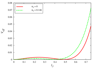
Figure 4: The $N=3$ effective potential, at the transition, for $\kappa_{3}=0$ (full line) and $0.146$ (dashed line).

To obtain the effective potential, we simply add the loop potential ${\cal V}$ to ${\cal V}_{V\!dm}$. The result for the three-color analogue of the Gross-Witten point, i.e. the potential from eq. (79) with all couplings $\kappa_{i}=0$, is depicted in Fig. 4 by the solid line. The value of the order parameter at the transition, $\ell_{0}^{+}\approx 0.485$, is very close to the $N=\infty$ value of $\frac{1}{2}$ dhlop ; kogut . Since the Vandermonde potential for $N=3$ is so close to $N=\infty$, this small shift, by $\approx 3\%$, is reasonable. Similarly, as can be seen graphically, the potential is almost flat at $T_{d}$. Masses are small at the transition, and there is a small barrier between degenerate minima of the potential. Physically, this corresponds to a nearly vanishing interface tension between phases.

As mentioned in the Introduction, lattice data for $SU(3)$ Yang-Mills indicates that $\ell_{0}(T_{d}^{+})$ is less than $\frac{1}{2}$, perhaps $\approx 0.4\pm 10\%$ dhlop . Additional lattice simulations are needed to fix the jump in the triplet loop more precisely. Nevertheless, in what follows we shall assume that $\ell_{0}^{+}=0.4$ to illustrate the effects of interactions.

We consider in detail adding a cubic term to the loop potential, $\kappa_{3}\neq 0$. We have also considered adding higher terms, such as a quartic term, $\kappa_{4}\neq 0$, but found numerically that the results are rather similar. With $\kappa_{3}\approx 0.146$, we obtain $\ell_{0}^{+}\approx 0.4$ for the triplet loop. The effective potential is shown in Fig. 4, and exhibits an even smaller barrier between the two phases than for $\kappa_{3}=0$.

Numerically, we also find that at the transition, the masses in the two minima are equal, to within a few percent, for both $\kappa_{3}=0$ and $=0.146$. This allows us to make the following observation. Any polynomial approximation to the potential fails for $\ell\approx 1$, due to a logarithmic term which represents eigenvalue repulsion. However, we can always use a polynomial approximation for small $\ell$. Consider a polynomial in $\ell$ to quartic order, of the form $\sim\ell^{2}(\ell-\ell_{0}^{+})^{2}$: this represents two degenerate minima, at $\ell=0$ and $\ell=\ell_{0}^{+}$. We find that at the transition, such a form is approximately valid for $\ell\leq 0.6$. Further, it is clear that this potential gives equal masses in both the confined and deconfined phases, which is nearly true numerically.

Such a quartic parametrization of the effective potential is, in fact, the basis for the Polyakov loop model banks_ukawa ; loop1 ; loop2a ; loop2b ; loop2c ; loop2d ; loop2e ; loop2f ; loop3 ; sannino ; ogilvie . The value of $\ell_{0}^{+}$ in the Polyakov loop model, $\approx.55$ loop2a , is close to that found from the lattice dhlop ; bielefeld . Moreover, the form of the potential is graphically very similar to that found in the matrix model, with an extremely small barrier between the two phases: see Fig. 1 of loop2a .

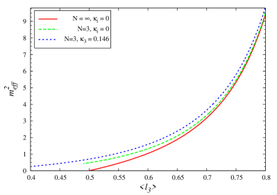
Figure 7: The effective mass squared, for the fundamental loop in the deconfined phase, versus its expectation value. The three curves are $N=\infty$ about the Gross-Witten point, all $\kappa_{i}=0$ (full line); $N=3$ with all $\kappa_{i}=0$ (dashed line); and $N=3$ with $\kappa_{3}=0.146$ (dotted line).

We also computed the effective mass in the matrix model. At infinite $N$, the value about the Gross–Witten point is given in eq. (50). For $N=3$, the effective mass is obtained numerically by computing the curvature of ${\cal V}_{e\!f\!f}$ about the non-trivial minimum $\ell_{0}$, cf. eq. (48). The results for $\kappa_{3}=0$ and $\kappa_{3}\neq 0$ are shown in Fig. 7 as a function of the expectation value of the fundamental loop. At the Gross-Witten point, $\ell_{0}(T_{d}^{+})=\frac{1}{2}$ and $m^{2}_{eff}(T_{d}^{+})=0$, as discussed in Sec. III.1. When $N=3$, at the transition the effective mass is small, but nonzero. In agreement with the discussion of ${\cal V}_{e\!f\!f}$ above, when $\kappa_{3}\neq 0$, both the expectation value of the triplet loop, and the effective mass, are smaller than for $\kappa_{3}=0$. Except for this small effect, for both values of $\kappa_{3}$ the effective mass for $N=3$ is close to that at infinite $N$. This happens because the Vandermonde potential at $N=3$ is close to $N=\infty$, and $\kappa_{3}=0.146$ is a small value. For example, since $\ell\approx\frac{1}{2}$ and $m^{2}\approx 1$ at the transition, the cubic coupling, $\kappa_{3}\ell^{3}$, is $\approx 8\%$ relative to the adjoint loop, $m^{2}\ell^{2}$.

To compute the expectation values of loops in higher representations we use a mean field analysis, like that of Sec. III.3 dhlop . We checked that for $\kappa_{3}=0$, the expectation value of the triplet loop, as computed from the effective potential, agrees with the mean field result. The expectation values of the loops in the triplet, sextet, octet, and decuplet representations of $SU(3)$, computed in this way, are shown in Fig. 5. We plot them as functions of the coupling $m^{2}$, divided by the critical value at which the transition occurs: $m^{2}_{\rm crit}\approx 0.91$ for $\kappa_{3}=0$, and $m^{2}_{\rm crit}\approx 0.97$ for $\kappa_{3}=0.146$. For $\kappa_{3}\neq 0$, the cubic term in the loop potential reduces the expectation values of all loops, not just that of the triplet loop. When $m^{2}\rightarrow\infty$, the effect of the cubic interaction diminishes, as the expectation values of all loops approach that for $\kappa_{3}=0$.

In agreement with the original results of dhlop , we find that the triplet loop, as measured on the lattice, agrees approximately with that for $\kappa_{3}=0.146$, assuming a linear relation between $m^{2}$ and the temperature about $T_{d}$. The lattice data is not sufficiently precise to make a detailed comparison, however. In particular, as the loop approaches one, this is not an accurate way of determining the relationship between $m^{2}$ and the temperature. We return to this point shortly.

For representations beyond the triplet, the difference loop, introduced in dhlop , is the remainder between the expectation value of the loop, and the result expected in the large $N$ limit, which is a product of fundamental (and anti-fundamental) loops:

$$\delta\ell_{\cal R}=\langle\ell_{\cal R}\rangle-\langle\ell_{3}\rangle^{p_{+}}\langle\ell_{3}^{*}\rangle^{p_{-}}\;.$$ (82)

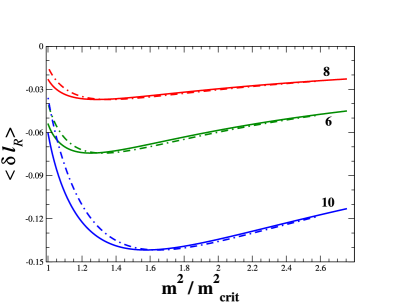
Figure 6: Difference loops for $6$, $8$, and $10$ representations of $SU(3)$, for $\kappa_{3}=0$ (full lines) and $0.146$ (dashed lines), as a function of the ratio of $m^{2}$ to its critical value.

The integers $(p_{+},p_{-})$ are $(2,0)$ for the sextet, $(1,1)$ for the octet, and $(3,0)$ for the decuplet representation. The difference loops are plotted in Fig. 6. Here, too, we find that the cubic interaction only matters near the transition: $\delta\ell_{8}$, $\delta\ell_{6}$ and $\delta\ell_{10}$ are slightly smaller in magnitude near $T_{d}$ when $\kappa_{3}>0$, relative to their values for $\kappa_{3}=0$.

In all cases, we find that the difference loops are much smaller than those measured on the lattice, Fig. 9 of dhlop . To make a detailed comparison, it is necessary to know the precise relation between the parameter $m^{2}$ of the matrix model and the temperature. Even without this relation, however, the sextet difference loop is about four times larger on the lattice than in the matrix model. For the octet difference loop, the lattice data exhibits a sharp spike close to the transition, about six times larger than the value in the matrix model. There is, as of yet, no data for the decuplet loop from the lattice. To describe these behaviors in a matrix model, it will certainly be necessary to include fluctuations, due to kinetic terms in the action. It is not apparent whether the lattice data can be fit with couplings and kinetic terms whose coefficients are independent of temperature.

We conclude by discussing the relationship of our results to the Polyakov loop model banks_ukawa ; loop1 ; loop2a ; loop2b ; loop2c ; loop2d ; loop2e ; loop2f ; loop3 ; sannino ; ogilvie . In this model, the pressure is assumed to be a potential for $\ell$ times $T^{4}$. As discussed above, this form does seem to work well near the transition. In order to fit the pressure away from $T_{d}$, however, it is necessary to assume that the variation of $m^{2}$ is not simply linear in the temperature. As shown in loop2d , by temperatures of $\approx 3T_{d}$, the pressure is nearly a constant times $T^{4}$; this requires that $m^{2}$ is nearly constant with respect to temperature. As noted above, when the value of the loop is near one, and given the uncertainties in the lattice data, we cannot exclude such a change in the relationship between $m^{2}$ and the temperature.

For $N=3$, assuming that the real part of the Polyakov loop condenses, one can compute masses for both the real and imaginary parts of the Polyakov loop loop2c . The effective masses discussed above refer only to that for the real part of the Polyakov loop. This is a (trivial) limitation of the matrix model, and is easiest to understand in the perturbative limit, when $m^{2}\rightarrow\infty$, so $\ell\rightarrow 1$. In this limit, ${\bf L}\approx\bf{1}+\sigma$, where $\sigma$ is an element of the Lie algebra, and the action is $\sim m^{2}\;{\rm tr}\;\sigma^{2}$. Integrating over $\sigma$, by (62) the effective mass is related to $1/m^{2}_{eff}\sim\int d\sigma\;({\rm tr}\;(\sigma^{2}))^{2}\exp(-m^{2}{\rm tr}\;\sigma^{2})$, and gives $m^{2}_{eff}\sim m^{4}$. This is the same behavior as at large $N$, as can be read off from (50) when $\ell_{0}\rightarrow 1$. If we do the same for the imaginary part of the loop, which starts as ${\rm Imag}({\rm tr}\;{\bf L})\sim{\rm tr}\;\sigma^{3}$, we would conclude that its effective mass squared is $\sim m^{6}$. This is wrong, however: in the full theory, the ratio between the effective mass for the imaginary, and real, parts of the fundamental loop must be $3/2$, as it is in the gauge theory in the perturbative limit. The problem, as noted by Brezin et al. brezin , is simply that because there are no kinetic terms, one cannot generally compute two point functions in a matrix model, but only one point functions. It is really exceptional that we could obtain even the mass for the real part of the fundamental loop. Of course, this is automatically remedied by adding kinetic terms to the matrix model.

V Conclusions

In this paper we developed a general approach to the deconfining transition, based upon a matrix model of Polyakov loops. The effective action for loops starts with a potential term. The Vandermonde determinant, which appears in the measure of the matrix model, also contributes a potential term.

At infinite $N$, the vacua are the stationary points of an effective potential, the sum of loop and Vandermonde potentials. Because of the Vandermonde potential, there is a transition with just a mass term, at the Gross–Witten point. This transition is of first order, but without an interface tension between the two phases. In the space of all possible potentials, which include arbitrary interactions of the Wilson line, the Gross–Witten point is exceptional. Away from it, the transitions appear ordinary, either of first order, with a nonzero jump of $\ell$ and nonvanishing masses, or of second order, with vanishing masses and no jump in the order parameter. (There are also third order transitions, with no jump in the order parameter and nonzero masses.) Only by tuning an infinite number of couplings to vanish does one reach the Gross–Witten point, where the order parameter jumps, and yet masses are zero.

We investigated the $N=3$ matrix model about the Gross–Witten point, including interactions. We found that the $N=3$ Vandermonde potential is very close to $N=\infty$, so that for small interactions, the $N=3$ effective potential strongly resembles that of infinite $N$. We found that in the $N=3$ matrix model, corrections to the large $N$ limit are small, $\sim 1/N$.

What is so surprising about the lattice data is that the $SU(3)$ deconfining transition is well described by a matrix model near the Gross–Witten point dhlop . In the confined phase, on the lattice the expectation value of the $Z(3)$ neutral octet loop was too small to measure; in a matrix model, it vanishes identically. At the transition, the renormalized triplet loop jumps to $\approx 0.4$  dhlop ; bielefeld , which is close to the Gross–Witten value of $\frac{1}{2}$. Further, masses associated with the triplet loop — especially the string tension — do decrease significantly near the transition three .

Of course, the proximity of the $SU(3)$ lattice data to the Gross–Witten point could be serendipitous, due to $N=3$ being close to the second order transition of $N=2$. For $N\geq 4$, the lattice does find a first order deconfining transition four_colors ; teper ; meyer . The lattice data also shows that at a fixed value of $T/T_{d}$, mass ratios increase with $N$. In the confined phase, one can compare the ratio of the temperature dependent string tension to its value at zero temperature. This can be done for $N=2$ two_colors_B , $3$ three , $4$ and $6$ teper ; meyer . For example, comparing $N=4$ and $6$, Fig. 5 of meyer shows that at fixed $T/T_{d}$, this ratio of string tensions increases as $N$ does. In the deconfined phase, Fig. 7 of the most recent work by Lucini, Teper, and Wenger teper shows that the ratio of the Debye mass at $T_{d}^{+}$, to $T_{d}$, is significantly larger for $N=8$ than for $N=3$. Thus, the lattice data strongly indicates that the $N=\infty$ theory is not exactly at the Gross–Witten point; if it were, at finite $N$ one would expect that mass ratios would decrease, as $T\rightarrow T_{d}$, in a manner which is nearly $N$-independent.

A recent, lengthy calculation by Aharony et al. shows that on a small sphere, at infinite $N$ the deconfining transition is of first order aharony3 . If $g$ is the gauge coupling, then as $N\rightarrow\infty$, $g^{2}N$ is a number of order one, while $g^{2}N\ll 1$ on a small sphere. In this limit, the coefficient of the quartic coupling in the loop potential, (63), is $\kappa_{4}\sim(g^{2}N)^{2}$ aharony ; aharony3 finds that $\kappa_{4}\approx-(1/10)(g^{2}N/(4\pi))^{2}$. Although it is difficult to know how to normalize the coefficient, its value suggests that on a small sphere, the theory is near the Gross–Witten point. Perhaps this remains true in an infinite volume.

With optimism, then, we assume that in the sense of Sec. III.5, the deconfining transition at $N=\infty$ is close to, but not at, the Gross–Witten point. We suggest that at finite $N$, fluctuations can drive the theory much closer to this point: that it is, in the space of all possible couplings, an infrared stable fixed point. Couplings only flow due to fluctuations, however, and in matrix models these are manifestly $\sim 1/N^{2}$. Thus this can only happen in a region of temperature which shrinks as $N$ increases, for $|T-T_{d}|/T_{d}\approx 1/N^{2}$.

A comparison of lattice simulations at different values of $N$ provides some evidence for a critical window which narrows with increasing $N$. Consider the decrease of the string tension near $T_{d}$. Define a temperature $T_{1/2}$ as the point at which the string tension is half its value at zero temperature, $\sigma(T_{1/2})\equiv 0.5\,\sigma(0)$. The lattice finds that the corresponding reduced temperature, $\delta t_{1/2}\equiv(T_{d}-T_{1/2})/T_{d}$, decreases as $N$ increases: $\delta t_{1/2}\approx 0.2$ at $N=2$ (Fig. 3 of two_colors_B ), $\approx 0.08$ when $N=3$ (Fig. 5 of three ), and $\approx 0.05$ for $N=4$ (Fig. 5 of meyer ). These three points can be fit with

$$\delta t_{1/2}\approx 0.8/N^{2}\;.$$ (83)

This really is a narrow window, with $\delta t_{1/2}\approx 0.02$ for $N=6$.

Unfortunately, a loop model cannot predict the ratio of the string tension at $T_{d}$, to zero temperature, because we do not know what $m^{2}$ corresponds to zero temperature. For three colors, this ratio is $\approx 0.12$ three . A loop model can predict the ratio of the string tension, to the Debye mass, at $T_{d}$. At infinite $N$, as $T\rightarrow T_{d}$ the string tension vanishes as $\sigma(T)\sim|T-T_{d}|^{1/2}$, while the Debye mass vanishes more slowly, $m_{Debye}\sim|T-T_{d}|^{1/4}$ (49) and (51) dhlop . That $\sigma(T)/m_{Debye}(T)\sim|T_{d}-T|^{1/4}$ as $T\rightarrow T_{d}$ is unlike ordinary second order transitions, where the analogous ratio is constant in a mean field approximation. For three colors, $\sigma(T_{d}^{-})/m_{Debye}(T_{d}^{+})\approx 0.93\pm 0.02$ at the $N=3$ analogy of the Gross–Witten point, and $\approx 0.99\pm 0.03$ when $\kappa_{3}=0.146$, Sec. IV.2. For four colors, it is $\approx 0.63\pm 0.02$ at the $N=4$ analogy of the Gross–Witten point mean , and decreases with increasing $N$.

The most direct way to test if the transition for $N\geq 4$ is close to the Gross–Witten point is to compute the value of the renormalized fundamental loop (very) near $T_{d}^{+}$ dhlop ; bielefeld , and see if it is close to $\frac{1}{2}$. The change in the masses near $T_{d}$ is probably more dramatic, though: since the latent heat grows as $\sim N^{2}$ teper ; meyer , such a decrease, especially in a window which narrows as $N$ increases, would be most unexpected.

To rigorously demonstrate the connection between loop models and deconfinement, it will be necessary to include fluctuations at finite $N$. At the beginning of Sec. III, we blithely ignored the kinetic terms of Sec. II.3, proceeding immediately to a mean field theory, which is an expansion in bare quantities. Including fluctuations will require the analysis of the renormalized theory. Fluctuations are most important in the lower critical dimension, which is two zinn ; beta , and is relevant for the deconfining transition in three spacetime dimensions threedim . The effect of fluctuations can also be computed by working down from the upper critical dimension, which is four. In this vein, we comment that the entire discussion of Sec. III is dominated by the Vandermonde potential, which arises from the measure of the matrix integral. In the continuum limit, terms in the measure can be eliminated from perturbation theory by the appropriate regulator zinn . The measure can contribute non-perturbatively, though: see, e.g., Eq. (73) of Billo, Caselle, D’Adda, and Panzeri largeN . In general, it will be interesting to develop the renormalization group for what may be a new universality class, about the Gross–Witten point.

Acknowledgements The research of A.D. is supported by the BMBF and the GSI; R.D.P., by the U.S. Department of Energy grant DE-AC02-98CH10886; J.T.L., by D.O.E. grant DE-FG02-97ER41027. R.D.P. also thanks: the Niels Bohr Institute, for their gracious hospitality during the academic year 2004-2005; the Alexander von Humboldt Foundation, for their support; K. Petrov, for discussions about three dimensions; P. Damgaard, for many discussions; and most especially, K. Splittorff, for frequent discussions, and for collaborating on part of the results in Secs. III and IV.

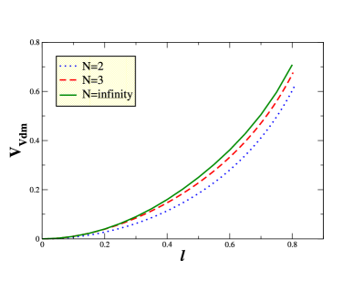
Figure 3: The Vandermonde potential, ${\cal V}_{Vdm}$, for $N=2$ (dotted line), $N=3$ (dashed line) and $N=\infty$ (full line).

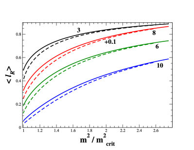
Figure 5: Expectation values for the $3$, $6$, $8$, and $10$ representations of $SU(3)$, for $\kappa_{3}=0$ (full lines) and $0.146$ (dashed lines), as a function of the ratio of $m^{2}$ to its critical value. For better visibility, the expectation value of the octet has been shifted by +0.1

References

- (1) G. ’t Hooft, Nucl. Phys. B 138, 1 (1978); ibid. 153, 141 (1979); A. M. Polyakov, Phys. Lett. B 72, 477 (1978); L. Susskind, Phys. Rev. D 20, 2610 (1979).
- (2) E. Laermann and O. Philipsen, [arXiv:hep-ph/0303042]; F. Karsch and E. Laermann, [arXiv:hep-lat/0305025].
- (3) A. Dumitru, Y. Hatta, J. Lenaghan, K. Orginos and R. D. Pisarski, Phys. Rev. D 70, 034511 (2004) [arXiv:hep-th/0311223].
- (4) O. Kaczmarek, F. Karsch, P. Petreczky, and F. Zantow, Phys. Lett. B 543, 41 (2002) [arXiv:hep-lat/0207002]; S. Digal, S. Fortunato, and P. Petreczky, [arXiv:hep-lat/0211029]; O. Kaczmarek, F. Karsch, P. Petreczky and F. Zantow, Nucl. Phys. Proc. Suppl. B 129, 560 (2004) [arXiv:hep-lat/0309121]; O. Kaczmarek, S. Ejiri, F. Karsch, E. Laermann and F. Zantow, [arXiv:hep-lat/0312015]; P. Petreczky and K. Petrov, [arXiv:hep-lat/0405009].
- (5) O. Philipsen, Phys. Lett. B 535, 138 (2002) [arXiv:hep-lat/0203018]; O. Jahn and O. Philipsen, [arXiv:hep-lat/0407042].
- (6) A. M. Polyakov, Nucl. Phys. B 164, 171 (1980); S.V. Ivanov, G.P. Korchemsky, A.V. Radyushkin, Sov. Jour. Nucl. Phys. 44, 145 (1986); G.P. Korchemsky and A.V. Radyushkin, Nucl. Phys. B 283, 342 (1987); Phys. Lett. B 279, 359 (1992); A. V. Belitsky, A. S. Gorsky and G. P. Korchemsky, Nucl. Phys. B 667, 3 (2003) [arXiv:hep-th/0304028].
- (7) For spatial separation , the renormalization constant for the Wilson loop at is a product of two terms, one for mass renormalization of the loop, , and one involving the cusps in the loop, . The first involves the product of the divergent mass times the total length of the loop: , where at lattice spacing dhlop . The latter involves the anomalous dimensions for the four cusps in a rectangular loop cusp : , where is the anomalous dimension for a cusp of , is the -function, and is the gauge coupling constant. There is no condition needed to fix at some scale, but one is needed for dhlop ; cusp . Straight Polyakov loops don’t have cusps (although one can construct “crooked” Polyakov loops which do dhlop ). The contribution of the anomalous dimensions for the four cusps may explain the persistent discrepancy, of , between the methods of dhlop , for the renormalized Polyakov loop, and that of bielefeld , for the renormalized Wilson loop at .
- (8) J. Engels and T. Scheideler, Phys. Lett. B 394, 147 (1997) [arXiv:hep-lat/9610019]; Nucl. Phys. B 539, 557 (1999) [arXiv:hep-lat/9808057].
- (9) S. Digal, S. Fortunato and P. Petreczky, Phys. Rev. D 68, 034008 (2003) [arXiv:hep-lat/0304017].
- (10) O. Kaczmarek, F. Karsch, E. Laermann and M. Lutgemeier, Phys. Rev. D 62, 034021 (2000) [arXiv:hep-lat/9908010].
- (11) S. Ohta and M. Wingate, Phys. Rev. D 63, 094502 (2001) [arXiv:hep-lat/0006016]; R. V. Gavai, Nucl. Phys. B 633, 127 (2002) [arXiv:hep-lat/0110054].
- (12) B. Lucini, M. Teper, and U. Wenger, Phys. Lett. B 545, 197 (2002) [arXiv:hep-lat/0206029]; Jour. High Energy Phys. 0401, 061 (2004) [arXiv:hep-lat/0307017]; [arXiv:hep-lat/0502003]; M. Teper, [arXiv:hep-th/0412005].
- (13) H. Meyer and M. Teper, Jour. High Energy Phys. 0412, 031 (2004) [arXiv:hep-lat/0411039].
- (14) J. O. Andersen and M. Strickland, [arXiv:hep-ph/0404164]; J. P. Blaizot, E. Iancu and A. Rebhan, [arXiv:hep-ph/0303185]; U. Kraemmer and A. Rebhan, Rep. Prog. Phys. 67, 351 (2004) [arXiv:hep-ph/0310337].
- (15) P. F. Kolb and U. Heinz, [arXiv:nucl-th/0305084]; E. V. Shuryak and I. Zahed, [arXiv:hep-ph/0307267]; G. E. Brown, C. H. Lee, M. Rho and E. Shuryak, [arXiv:hep-ph/0312175]; E. V. Shuryak and I. Zahed, [arXiv:hep-ph/0403127]; M. Gyulassy and L. McLerran, [arXiv:nucl-th/0405013]; U. Heinz, [arXiv:hep-ph/0407360].
- (16) N. Cabibbo and G. Parisi, Phys. Lett. B 59, 67 (1975); B. S. Skagerstam, Z. Phys. C 24, 97 (1984); B. Sundborg, Nucl. Phys. B 254, 583 (1985); J. J. Atick and E. Witten, Nucl. Phys. B 310, 291 (1988);
- (17) J. Hallin and D. Persson, Phys. Lett. B 429, 232 (1998) [arXiv:hep-ph/9803234]; B. Sundborg, Nucl. Phys. B 573, 349 (2000) [arXiv:hep-th/9908001].
- (18) O. Aharony, J. Marsano, S. Minwalla, K. Papadodimas, and M. Van Raamsdonk, [arXiv:hep-th/0310285], v.5.
- (19) K. Furuuchi, E. Schreiberg, and G. Semenoff, [arXiv:hep-th/0310286].
- (20) H. J. Schnitzer, [arXiv:hep-th/0402219].
- (21) O. Aharony, J. Marsano, S. Minwalla and T. Wiseman, [arXiv:hep-th/0406210]; H. Liu, [arXiv:hep-th/0408001]; M. Spradlin and A. Volovich, [arXiv:hep-th/0408178].
- (22) T. Banks and A. Ukawa, Nucl. Phys. B 225, 145 (1983).
- (23) R. D. Pisarski, Phys. Rev. D 62, 111501 (2000) [arXiv:hep-ph/0006205].
- (24) A. Dumitru and R. D. Pisarski, Phys. Lett. B 504, 282 (2001) [arXiv:hep-ph/0010083].
- (25) A. Dumitru and R. D. Pisarski, Phys. Lett. B 525, 95 (2002) [arXiv:hep-ph/0106176].
- (26) A. Dumitru and R. D. Pisarski, Phys. Rev. D 66, 096003 (2002) [arXiv:hep-ph/0204223].
- (27) O. Scavenius, A. Dumitru and J. T. Lenaghan, Phys. Rev. C 66, 034903 (2002) [arXiv:hep-ph/0201079]; A. Dumitru, O. Scavenius, and A. D. Jackson, Phys. Rev. Lett. 87, 182302 (2001) [arXiv:hep-ph/0103219].
- (28) A. Dumitru, D. Röder and J. Ruppert, [arXiv:hep-ph/0311119].
- (29) R. D. Pisarski, [arXiv:hep-ph/0203271], and references therein.
- (30) I. I. Kogan, A. Kovner and J. G. Milhano, Jour. High Energy Phys. 0212, 017 (2002) [arXiv:hep-ph/0208053]; K. Fukushima, ibid. 68, 045004 (2003) [arXiv:hep-ph/0303225]; [arXiv:hep-ph/0310121]; Y. Hatta and K. Fukushima, [arXiv:hep-ph/0307068]; [arXiv:hep-ph/0311267].
- (31) A. Mocsy, F. Sannino and K. Tuominen, Phys. Rev. Lett. 91, 092004 (2003) [arXiv:hep-ph/0301229]; Jour. High Energy Phys. 0403, 044 (2004) [arXiv:hep-ph/0306069]; [arXiv:hep-ph/0308135]; F. Sannino and K. Tuominen, [arXiv:hep-ph/0403175].
- (32) P. N. Meisinger, T. R. Miller, and M. C. Ogilvie, Phys. Rev. D 65, 034009 (2002) [arXiv:hep-ph/0108009]; P. N. Meisinger and M. C. Ogilvie, Phys. Rev. D 65, 056013 (2002) [arXiv:hep-ph/0108026]; P. N. Meisinger and M. C. Ogilvie, [arXiv:hep-ph/0409136]; M. Schaden, [arXiv:hep-th/0410254].
- (33) D. J. Gross, R. D. Pisarski and L. G. Yaffe, Rev. Mod. Phys. 53, 43 (1981); N. Weiss, Phys. Rev. D 25, 2667 (1982); K. Enqvist and K. Kajantie, Z. Phys. C 47, 291 (1990); V. M. Belyaev and V. L. Eletsky, Z. Phys. C 45, 355 (1990) [Sov. J. Nucl. Phys. 51, 168 (1990)]; V. M. Belyaev, Phys. Lett. B 254, 153 (1991).
- (34) T. Bhattacharya, A. Gocksch, C. Korthals Altes and R. D. Pisarski, Phys. Rev. Lett. 66, 998 (1991); Nucl. Phys. B 383, 497 (1992) [arXiv:hep-ph/9205231]; S. Chapman, Phys. Rev. D 50, 5308 (1994) [arXiv:hep-ph/9407313]; J. Wirstam, Phys. Rev. D 65, 014020 (2002) [arXiv:hep-ph/0106141]; P. Giovannangeli and C. P. Korthals Altes, Nucl. Phys. B 608, 203 (2001) [arXiv:hep-ph/0102022]; [arXiv:hep-ph/0212298]; [arXiv:hep-ph/0412322]; D. Diakonov and M. Oswald, Phys. Rev. D 68, 025012 (2003) [arXiv:hep-ph/0303129]; [arXiv:hep-ph/0312126]; [arXiv:hep-ph/0403108]; E. Megias, E. Ruiz Arriola and L. L. Salcedo [arXiv:hep-ph/0312133].
- (35) J. Zinn-Justin, “Quantum Field Theory and Critical Phenomena” (Clarendon Press, Oxford, 1997).
- (36) J. M. Drouffe and J. B. Zuber, Phys. Rep. 102, 1 (1983).
- (37) S. R. Das, Rev. Mod. Phys. 59, 235 (1987); P. Di Francesco, P. H. Ginsparg and J. Zinn-Justin, Phys. Rep. 254, 1 (1995) [arXiv:hep-th/9306153]; R. C. Brower, M. Campostrini, K. Orginos, P. Rossi, C. I. Tan and E. Vicari, Phys. Rev. D 53, 3230 (1996) [arXiv:hep-th/9508015]; P. Rossi, M. Campostrini and E. Vicari, Phys. Rep. 302, 143 (1998); [arXiv:hep-lat/9609003]; M. Billo, M. Caselle, A. D’Adda and S. Panzeri, Intl. Jour. Mod. Phys. A12, 1783 (1997) [arXiv:hep-th/9610144]; Yu. Makeenko, [arXiv:hep-th/0001047]; M. R. Douglas, I. R. Klebanov, D. Kutasov, J. Maldacena, E. Martinec and N. Seiberg, [arXiv:hep-th/0307195].
- (38) E. Brezin, C. Itzykson, G. Parisi and J. B. Zuber, Comm. Math. Phys. 59, 35 (1978).
- (39) D. J. Gross and E. Witten, Phys. Rev. D 21, 446 (1980).
- (40) J. Jurkiewicz and K. Zalewski, Nucl. Phys. B 220, 167 (1983).
- (41) J. B. Kogut, M. Snow, and M. Stone, Nucl. Phys. B 200, 211 (1982).
- (42) F. Green and F. Karsch, Nucl. Phys. B 238, 297 (1984).
- (43) P. H. Damgaard and A. Patkos, Phys. Lett. B 172, 369 (1986).
- (44) P. H. Damgaard, Phys. Lett. B 194, 107 (1987); J. Christensen and P. H. Damgaard, Phys. Rev. Lett. 65, 2495 (1990); Nucl. Phys. B 348, 226 (1991); ibid. 354, 339 (1991); J. Christensen, G. Thorleifsson, P. H. Damgaard and J. F. Wheater, Phys. Lett. B 276, 472 (1992); Nucl. Phys. B 374, 225 (1992); P. H. Damgaard and M. Hasenbusch, Phys. Lett. B 331, 400 (1994) [arXiv:hep-lat/9404008].
- (45) J. Kiskis, Phys. Rev. D 41, 3204 (1990).
- (46) J. F. Donoghue, E. Golowich, and B. R. Holstein, “Dynamics of the Standard Model” (Cambridge University Press, Cambridge, 1992).
- (47) J. Gasser and H. Leutwyler, Phys. Lett. B 188, 477 (1987); H. Leutwyler and A. Smilga, Phys. Rev. D 46, 5607 (1992); recent work includes: G. Akemann, J. T. Lenaghan and K. Splittorff, Phys. Rev. D 65, 085015 (2002) [arXiv:hep-th/0110157]; J. Lenaghan and T. Wilke, Nucl. Phys. B 624, 253 (2002) [arXiv:hep-th/0108166]; P. H. Damgaard, M. C. Diamantini, P. Hernandez and K. Jansen, Nucl. Phys. B 629, 445 (2002) [arXiv:hep-lat/0112016]; P. H. Damgaard, P. Hernandez, K. Jansen, M. Laine and L. Lellouch, ibid. 656, 226 (2003) [arXiv:hep-lat/0211020]; L. Giusti, M. Luscher, P. Weisz and H. Wittig, Jour. High Energy Phys. 0311, 023 (2003) [arXiv:hep-lat/0309189].
- (48) R. D. Pisarski, Phys. Rev. D 20, 3358 (1979).
- (49) R. D. Pisarski and M. Oswald, unpublished.
- (50) A. Dumitru, R. D. Pisarski, and D. Zschiesche, unpublished.
- (51) O. Aharony, J. Marsano, S. Minwalla, K. Papadodimas, and M. Van Raamsdonk, [arXiv:hep-th/0502149].
- (52) P. Bialas, A. Morel, B. Petersson, K. Petrov and T. Reisz, Nucl. Phys. B 581, 477 (2000) [arXiv:hep-lat/0003004]; ibid. 603, 369 (2001) [arXiv:hep-lat/0012019]; K. Petrov, [arXiv:hep-lat/0211028]; P. Bialas, A. Morel and B. Petersson, ibid. 704, 208 (2005) [arXiv:hep-lat/0403027].