Abstract

We study a particular texture of the neutrino mass matrix generated in supergravity with bilinear R-Parity violation. The relatively high value of $\tan\beta$ makes the one-loop contribution to the neutrino mass matrix as important as the tree-level one. The atmospheric angle is nearly maximal, and its deviation from maximal mixing is related to the smallness of the ratio between the solar and atmospheric mass scales. There is also a common origin for the small values of the solar and reactor angles, but the later is much smaller due the large mass ratio between the lightest two neutrinos. There is a high dependence of the neutrino mass differences on the scalar mass $m_{0}$ and the gaugino mass $M_{1/2}$, but a smaller one of the mixing angles on the same sugra parameters. Measurements of branching ratios for the neutralino decays can give important information on the parameters of the model. There are good prospects at a future Linear Collider for these measurements, but a more detailed analysis is necessary for the LHC.

1 Introduction

With a number of experimental results in atmospheric, solar, reactor, and accelerator neutrino physics, it has been established that neutrinos have mass and oscillate exp . This is a very important result in its own but, in addition, it is the first direct experimental indication that the Standard Model (SM) needs to be modified Grimus:2003es .

In the SM neutrinos are massless. One popular mechanism for the generation of neutrino masses is the see-saw mechanism, where a right handed neutrino field with a very large mass is added to the SM seesaw . The resulting neutrino mass is inversely proportional to this large mass. Another interesting and predictive mechanism is the radiative generation of neutrino masses and mixing in a supersymmetric model Hirsch:2004he that violates lepton number and R-Parity Farrar:xj with bilinear terms in the superpotential. Phenomenological consequences of R-Parity violating supersymmetry are very distinct from R-Parity conserving models Chemtob:2004xr .

Bilinear R-Parity breaking is an interesting mechanism for the generation of neutrino masses and mixing angles due to its simplicity and predictability Akeroyd:1997iq , Carvalho:2002bq . It is a simple extension of the Minimal Supersymmetric Standard Model (MSSM) which includes no new fields and no new interactions. It differs from the MSSM in a handful of bilinear terms that violate lepton number and R-Parity, which cannot be eliminated with field redefinitions Diaz:1998vf . Neutrino masses and mixing angles are calculable and agree with experimental measurements Romao:1999up , Hirsch:2000ef . Motivations for BRpV are for example, models with spontaneously broken R-Parity Nogueira:1990wz , and a model with an anomalous horizontal $U(1)$ symmetry Mira:2000gg , where BRpV appears without trilinear R-Parity violation.

Results from SuperKamiokande exp on atmospheric neutrinos gave strong evidence of the $\nu_{\mu}-\nu_{\tau}$ oscillation of the atmospheric neutrinos with maximal or nearly maximal mixing, and gave strong evidence against the small mixing angle solution of the solar neutrino problem. Results from the Sudbury Neutrino Observatory (SNO) and the KamLAND experiment have confirmed the large mixing angle solution of the solar neutrino problem, showing that more than a half of the electron-neutrinos produced at the sun oscillate into other flavours before reaching Earth exp . Results from the Wilkinson Microwave Anisotropy Probe (WMAP) show temperature differences within the microwave background radiation, which combined with results from large scale structure give a bound on the sum of the neutrino masses Kogut:2003et . Finally, evidence for neutrinoless double beta decay, if confirmed, would show the Majorana nature of neutrinos and the non-conservation of lepton numbers Klapdor-Kleingrothaus:2001ke .

There are several analysis of these experimental results Nunokawa:2002mq . The $3\sigma$ allowed regions for the neutrino parameters in Maltoni:2004ei are

$$1.4\times 10^{-3}< \Delta m^{2}_{32} <3.3\times 10^{-3}\,{\mathrm{eV}}^{2}$$

$$7.2\times 10^{-5}< \Delta m^{2}_{21} <9.1\times 10^{-5}\,{\mathrm{eV}}^{2}$$

$$0.52< \tan^{2}\theta_{23} <2.1$$ (1)

$$0.30< \tan^{2}\theta_{12} <0.61$$

$$\tan^{2}\theta_{13} <0.049$$

which we show for reference.

In this article, we re-analyze the possibility of having BRpV in a supergravity scenario, in which the scalar masses and the gaugino masses are universal at the GUT scale. The electroweak symmetry is broken radiatively but, contrary to the MSSM, sneutrinos acquire vacuum expectation values as well as the Higgs bosons. We give up the possibility that the $\epsilon_{i}$ and $B_{i}$ parameters (one for each lepton and analogous to the $\mu$ and $B$ term in the MSSM respectively) are universal at the GUT scale, because otherwise there is no good solution for the neutrino physics compatible with experiments.

We found solutions that have not been discussed previously in the literature. These solutions are characterized by a large value of $\tan\beta$ and, therefore, the importance of one-loop contributions to the neutrino mass matrix is enhanced.

2 Neutrino Mass at Tree Level

The superpotential of our BRpV model differs from the MSSM by three terms which violate R-Parity and lepton number,

$$W=W_{MSSM}+\epsilon_{i}\hat{L}_{i}\hat{H}_{u}$$ (2)

where $\epsilon_{i}$ have units of mass. We complement them with related terms in the soft lagrangian,

$${\cal L}={\cal L}_{MSSM}+B_{i}\epsilon_{i}\widetilde{L}_{i}H_{u}$$ (3)

where $B_{i}$ also have units of mass. The presence of these terms induce vacuum expectation values $v_{i}$ for the sneutrinos, which are calculated minimizing the scalar potential.

At tree level neutrino masses are generated via a low energy see-saw type mechanism. Neutrinos mix with neutralinos, and the MSSM neutralino mass matrix is expanded to a $7\times 7$ mass matrix for the neutral fermions

$${\bf M}_{N}=\left[\matrix{{\cal M}_{\chi^{0}}&m^{T}\cr m&0}\right]$$ (4)

Here, ${\cal M}_{\chi^{0}}$ is the usual $4\times 4$ neutralino mass matrix, and $m$ is

$$m=\left[\begin{array}[]{cccc}-\frac{1}{2}g^{\prime}v_{1}&\frac{1}{2}gv_{1}&0&\epsilon_{1}\cr-\frac{1}{2}g^{\prime}v_{2}&\frac{1}{2}gv_{2}&0&\epsilon_{2}\cr-\frac{1}{2}g^{\prime}v_{3}&\frac{1}{2}gv_{3}&0&\epsilon_{3}\cr\end{array}\right]$$ (5)

which mixes the neutrinos with the neutralinos. The matrix ${\bf M}_{N}$ can be diagonalized by blocks, and the effective $3\times 3$ neutrino mass matrix turns out to be equal to

$${\bf M}_{\nu}^{(0)}=-m\cdot{\cal M}_{\chi^{0}}^{-1}\cdot m^{T}=\frac{M_{1}g^{2}\!+\!M_{2}{g^{\prime}}^{2}}{4\,det({\cal M}_{\chi^{0}})}\left[\matrix{\Lambda_{1}^{2}&\Lambda_{1}\Lambda_{2}&\Lambda_{1}\Lambda_{3}\cr\Lambda_{1}\Lambda_{2}&\Lambda_{2}^{2}&\Lambda_{2}\Lambda_{3}\cr\Lambda_{1}\Lambda_{3}&\Lambda_{2}\Lambda_{3}&\Lambda_{3}^{2}}\right]$$ (6)

where we have defined the parameters $\Lambda_{i}=\mu v_{i}+\epsilon_{i}v_{d}$, which are proportional to the sneutrino vacuum expectation values in the basis where the $\epsilon$ terms are removed from the superpotential.

This mass matrix can be diagonalized with the following two rotations.

$$V_{\nu}^{(0)}=\left(\begin{array}[]{ccc}1&0&0\\ 0&\cos\theta_{23}^{(0)}&-\sin\theta_{23}^{(0)}\\ 0&\sin\theta_{23}^{(0)}&\cos\theta_{23}^{(0)}\end{array}\right)\times\left(\begin{array}[]{ccc}\cos\theta_{13}^{(0)}&0&-\sin\theta_{13}^{(0)}\\ 0&1&0\\ \sin\theta_{13}^{(0)}&0&\cos\theta_{13}^{(0)}\end{array}\right),$$ (7)

where the reactor mixing angle in terms of the alignment vector ${\vec{\Lambda}}$ is

$$\tan\theta_{13}^{(0)}=-\frac{\Lambda_{1}}{(\Lambda_{2}^{2}+\Lambda_{3}^{2})^{\frac{1}{2}}},$$ (8)

and the atmospheric angle is

$$\tan\theta_{23}^{(0)}=\frac{\Lambda_{2}}{\Lambda_{3}}.$$ (9)

As we will see later, despite the fact that tree level contribution to the heavy neutrino mass dominates over all loops, there are other contributions to the neutrino mass matrix that cannot be neglected. For this reason, the above tree level formulas will not be enough to explain the results.

3 Supergravity and BRpV

In Sugra-BRpV the independent parameters are

$$m_{0}\,,M_{1/2}\,,A_{0}\,,\tan\beta\,,\mathrm{sign}(\mu)\,,\epsilon_{i}\,,\Lambda_{i}\,,$$ (10)

where $m_{0}$ is the universal scalar mass, $M_{1/2}$ is the universal gaugino mass, and $A_{0}$ is the universal trilinear coupling, valid at the GUT scale. In addition, $\tan\beta$ is the ratio between the Higgs vacuum expectation values, and ${\mathrm{sign}}(\mu)$ is the sign of the higgsino mass parameter, both valid at the EWSB scale. Finally, $\epsilon_{i}$ are the supersymmetric BRpV parameters in the superpotential, and $\Lambda_{i}$ are the parameters depending on the sneutrino vacuum expectation values.

We use the code SUSPECT Djouadi:2002ze to run the two loops RGE from the unification scale down to the weak scale. The electroweak symmetry breaking is analogous to the MSSM, with the difference that there are three extra vacuum expectation values corresponding to the sneutrino vev’s $v_{i}$. These vev’s are small and constitute a small perturbation to the MSSM EWSB.

Despite the fact that sneutrino vev’s are dependent quantities since they are calculated from the minimization of the scalar potential, we remove from the group of independent parameters the $B_{i}$’s in favour of $\Lambda_{i}=\mu v_{i}+\epsilon_{i}v_{d}$ as indicated in eq. (10), because they are more useful in describing the neutrino physics.

Our analysis will be centered around the SPS1 scenario in Sugra from the Snowmass 2001 benchmark scenarios Ghodbane:2002kg , which is defined by

$$m_{0}=100\,{\mathrm{GeV}}\,,\,M_{1/2}=250\,{\mathrm{GeV}}\,,\,A_{0}=-100\,{\mathrm{GeV}}\,,\,\tan\beta=10\,,\,\mu>0$$ (11)

This scenario is typical of Sugra, with a neutralino LSP with a mass $m_{\chi^{0}_{1}}=99$ GeV, and a light neutral Higgs boson with a mass just above the experimental limit $m_{h}=114$ GeV.

In this context we find several solutions for neutrino physics which satisfy the experimental constraints on the atmospheric and solar mass squared differences, the three mixing angles, and the mass parameter associated with neutrino-less double beta decay Klapdor-Kleingrothaus:2003rv . For illustrative purposes we single out the following

$$\epsilon_{1}=-0.0004\,,\, \epsilon_{2}=0.052\,,\, \epsilon_{3}=0.051\,,\,$$

$$\Lambda_{1}=0.022\,,\, \Lambda_{2}=0.0003\,,\, \Lambda_{3}=0.039\,,\,$$ (12)

This solution is characterized by

$$\Delta m^{2}_{32}=2.7\times 10^{-3}\,{\mathrm{eV}}^{2}\,, \Delta m^{2}_{21}=8.1\times 10^{-5}\,{\mathrm{eV}}^{2}\,, m_{ee}=0.0036\,{\mathrm{eV}}$$

$$\tan^{2}\theta_{23}=0.72\,, \tan^{2}\theta_{12}=0.54\,, \tan^{2}\theta_{13}=0.0058$$ (13)

which are well inside the experimentally allowed window in eq. (1). We note that the random solution in eq. (12) is compatible with $\epsilon_{1}=\Lambda_{2}=0$, i.e., the neutrino parameters in eq. (13) are hardly changed with this replacement.

4 Texture of Neutrino Mass Matrix

Among the solutions to neutrino physics that we have found in our model, there are a few textures Smirnov:2004ju for the effective neutrino mass matrix. Our study case in eq. (12) belongs to the most frequent one, which is

$${\bf M}^{eff}_{\nu}=m\left[\matrix{\lambda&0&\lambda\cr 0&a&a\cr\lambda&a&1}\right]$$ (14)

with $a\sim 0.5-0.8$, $\lambda\sim 0.1-0.3$, and $m\sim 0.02-0.04$ eV. To understand how this texture works we expand the neutrino masses and mixing angles in powers of $\lambda$. Keeping terms up to first order, the three neutrino masses are

$$m_{\nu_{1}} = \lambda m+{\cal O}(\lambda^{2})$$ (15)

$$m_{\nu_{2}} = {\textstyle{1\over 2}}m(1+a-\sqrt{5a^{2}-2a+1})+{\cal O}(\lambda^{2})$$ (16)

$$m_{\nu_{3}} = {\textstyle{1\over 2}}m(1+a+\sqrt{5a^{2}-2a+1})+{\cal O}(\lambda^{2})$$ (17)

and the rotation matrix that diagonalizes the neutrino mass matrix, denoted $U_{PMNS}$, is

$$U_{PMNS}=\left[\matrix{1&\lambda s_{\theta}m/m_{\nu_{2}}&\lambda c_{\theta}m/m_{\nu_{3}}\cr\lambda/(1-a)&c_{\theta}&-s_{\theta}\cr-\lambda/(1-a)&s_{\theta}&c_{\theta}}\right]+{\cal O}(\lambda^{2})$$ (18)

with

$$\tan 2\theta=\frac{-2a}{1-a}\,.$$ (19)

In the same approximation, the atmospheric, solar, and reactor angles are given by

$$\tan 2\theta_{23} = 2a/(1-a)+{\cal O}(\lambda^{2})$$ (20)

$$\tan\theta_{12} = \lambda s_{\theta}m/m_{\nu_{2}}+{\cal O}(\lambda^{2})$$ (21)

$$\sin\theta_{13} = \lambda c_{\theta}m/m_{\nu_{3}}+{\cal O}(\lambda^{2})$$ (22)

while the atmospheric and solar mass differences are

$$\Delta m_{32}^{2} = m^{2}(1+a)\sqrt{5a^{2}-2a+1}+{\cal O}(\lambda^{2})$$ (23)

$$\Delta m_{21}^{2} = {\textstyle{1\over 2}}m^{2}\left[1+3a^{2}-(1+a)\sqrt{5a^{2}-2a+1}\right]+{\cal O}(\lambda^{2})\,.$$ (24)

As an example, consider $a=1/2$ and $m=0.04$ eV. We find $\Delta m^{2}_{32}=3\sqrt{5}m^{2}/4\approx 2.7\times 10^{-3}\,{\mathrm{eV}}^{2}$, and $\Delta m^{2}_{21}=(7-3\sqrt{5})m^{2}/8\approx 5.8\times 10^{-5}\,{\mathrm{eV}}^{2}$, both in agreement with experiments. The third parameter which in this approximation does not depend on the small parameter $\lambda$ is the atmospheric angle, obtaining $\tan^{2}\theta_{23}\approx 0.4$ from eq. (19). This value is at the lower end of the allowed region, nevertheless, taking $a=0.6$ we obtain $\tan^{2}\theta_{23}\approx 0.5$, which is in better agreement with experiments.

The fact that $a$ is smaller than unity implies that the atmospheric mixing is not maximal. In the limit $a\rightarrow 1$, the atmospheric mixing approaches maximality, but the atmospheric mass $\Delta m^{2}_{atm}\rightarrow 4m^{2}$ which is too large if $m=0.04$ eV, and the solar mass $\Delta m^{2}_{sol}\rightarrow 0$ which is too small. Decreasing $\tan^{2}\theta_{atm}$ via decreasing $a$ will decrease the atmospheric mass scale and increase the solar one, both towards acceptable values. Therefore, the value of $a$ relates these three neutrino parameters, such that the non-maximal value for the atmospheric angle is connected to the smallness of the ratio between the solar mass scale and the atmospheric one.

The previous considerations are modified by the non zero value of $\lambda$. In the approximation we are working, the solar and reactor angles are proportional to the parameter $\lambda$, thus they are small quantities themselves. Nevertheless, the presence of $m_{\nu_{2}}$ in the denominator of $\tan\theta_{12}$ as opposed to $m_{\nu_{3}}$ in the denominator of $\tan\theta_{13}$, makes the reactor angle much smaller than the solar angle. In the case $a=1/2$ and $\lambda=0.2$ we find for the solar angle $\tan^{2}\theta_{12}=0.3$, which is in the lower part of the allowed region and compatible with experiments. For the reactor angle we find $\tan^{2}\theta_{13}=0.017$ which is well below the experimental upper bound. We stress that we use the complete numerical calculation in the rest of the article, rather than these approximated formulas.

5 One Loop Contributions

All particles in the MSSM contribute to the renormalization of the neutralino/neutrino mass matrix. One of the most important contributions comes from the bottom-sbottom loops. In the gauge eigenstate basis this contribution is Diaz:2003as ,

$$\Delta\Pi_{ij}=-{{N_{c}m_{b}}\over{16\pi^{2}}}2s_{\tilde{b}}c_{\tilde{b}}h_{b}^{2}\Delta B_{0}^{\tilde{b}_{1}\tilde{b}_{2}}\left[{{\epsilon_{i}\epsilon_{j}}\over{\mu^{2}}}-\frac{a_{3}}{\mu}\left(\epsilon_{i}\Lambda_{j}+\epsilon_{j}\Lambda_{i}\right)+\left(a_{3}^{2}+\frac{a_{L}a_{R}}{h^{2}_{b}}\right)\Lambda_{i}\Lambda_{j}\right]$$ (25)

where we have defined

$$a_{R}={g\over{\sqrt{2}}}\left({1\over 3}t_{W}a_{1}-a_{2}\right)\,,\qquad a_{L}={g\over{\sqrt{2}}}\,{2\over 3}t_{W}a_{1}$$ (26)

$$a_{1}={{g^{\prime}M_{2}\mu}\over{2\Delta_{0}}}\,,\quad a_{2}=-{{gM_{1}\mu}\over{2\Delta_{0}}}\,,\quad a_{3}=\frac{v_{u}}{4\Delta_{0}}(g^{2}M_{1}+g^{\prime 2}M_{2})\,,$$ (27)

The main contributions to eq. (25) can be understood as coming from the graph

Here, neutrinos (in the gauge eigenstate basis) mix with Higgsinos who in turn interact with the pair bottom-sbottom with a strength proportional to the corresponding Yukawa coupling. Full circles indicate the projection of the sbottom mass eigenstate into right and left sbottom, which contribute with a $\sin\theta_{\tilde{b}}$ and $\cos\theta_{\tilde{b}}$ respectively. Open circles indicate the projection of the neutrino field onto the higgsino, proportional to the small parameter $a_{3}\Lambda_{i}-\epsilon_{i}/\mu$. The quark propagator contributes with a factor $m_{b}$, and summing over color gives the factor $N_{c}$. Finally, we have in eq. (25)

$$\Delta B_{0}^{\tilde{b}_{1}\tilde{b}_{2}}\equiv B_{0}(0,m^{2}_{\tilde{b}_{1}},m^{2}_{b})-B_{0}(0,m^{2}_{\tilde{b}_{2}},m^{2}_{b})$$ (28)

The one-loop corrected neutrino mass matrix, in first approximation, has the general form

$$\Delta\Pi_{ij}=A\Lambda_{i}\Lambda_{j}+B(\epsilon_{i}\Lambda_{j}+\epsilon_{j}\Lambda_{i})+C\epsilon_{i}\epsilon_{j}$$ (29)

since all loop contributions can be expanded in this way. The terms of higher order in $\Lambda$ and $\epsilon$ have been neglected.

Considering the solutions to neutrino physics whose effective neutrino mass matrix has a texture of the form in eq. (14), and including contributions from all one-loop graphs, we extract the numerical value of the above parameters and find $A\approx 7\,{\mathrm{eV/GeV}}^{4}$, $B\approx-0.5\,{\mathrm{eV/GeV}}^{3}$, and $C\approx 9\,{\mathrm{eV/GeV}}^{2}$.

Of the three parameters only $A$ gets a contribution at tree level, and we estimate

$$A^{(0)}=\frac{g^{2}M_{1}+g^{\prime 2}M_{2}}{4\Delta_{0}}\approx 7.6\,{\mathrm{eV/GeV}}^{4}$$ (30)

Clearly, the tree level contribution to $A$ dominates over all one-loop graphs. This is not true for $B$ and $C$ because this two parameters are entirely generated at one-loop.

The contribution to $A$, $B$, and $C$ from the bottom-sbottom loops can be read from eq. (25). In the squark sector we have $m_{\tilde{b}_{1}}=492$, $m_{\tilde{b}_{2}}=538$ GeV, and $\sin 2\theta_{\tilde{b}}=0.88$, which implies

$$C^{(1)}_{\tilde{b}}=-{{N_{c}m_{b}}\over{8\pi^{2}\mu^{2}}}s_{\tilde{b}}c_{\tilde{b}}h_{b}^{2}\Delta B_{0}^{\tilde{b}_{1}\tilde{b}_{2}}\approx 9.8\,{\mathrm{eV/GeV}}^{2}$$ (31)

This result is very close to the actual numerical value, and underlines the fact that the bottom-sbottom loops are very important in this particular scenario.

Considering that the value for $B$, in the supergravity model we are working with, is much smaller than $A$ and $C$, we might in first approximation neglect it in eq. (29). In this case, for the neutrino solution in eq. (12) we obtain the following approximated neutrino mass matrix,

$${\bf M}^{eff}_{\nu}=\left[\matrix{A\Lambda_{1}^{2}&0&A\Lambda_{1}\Lambda_{3}\cr 0&C\epsilon_{2}^{2}&C\epsilon_{2}\epsilon_{3}\cr A\Lambda_{1}\Lambda_{3}&C\epsilon_{2}\epsilon_{3}&A\Lambda_{3}^{2}+C\epsilon_{3}^{2}}\right]$$ (32)

This form is precisely the texture observed in eq. (14) obtained from the numerical results. Therefore, the zero in the neutrino mass matrix is there because $\Lambda_{2},\epsilon_{1}\approx 0$ and because $B$ is very small compared with $A$ and $C$. The three matrix elements of order $\lambda$ in eq. (14) are explained by the fact that $\Lambda_{1}$ has a numerical value smaller than the other three relevant parameters, as can be seen from eq. (12). Finally, the parameter $a$ in eq. (14) is smaller than unity because $A\Lambda_{3}^{2}$ and $C\epsilon_{3}^{2}$ are comparable and of the same sign and because $\epsilon_{2}\approx\epsilon_{3}$.

6 Numerical Results

In this section we study numerical results on the neutrino mass matrix, neutrino mass differences and mixing angles. We center our studies in the supergravity benchmark given in eq. (11), although we also explore the behavior of the neutrino parameters in the $m_{0}-M_{1/2}$ plane. We look for solutions to neutrino physics with different values of the BRpV parameters $\epsilon_{i}$ and $\Lambda_{i}$, but concentrate our attention in the particular solution given in eq. (12).

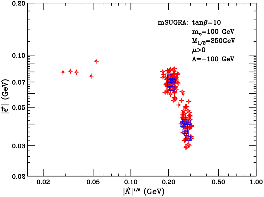
Figure 1: Solutions to neutrino physics passing all experimental cuts described in the text, working within a particular supergravity benchmark.

First, we consider the supergravity benchmark in eq. (11) and randomly vary the BRpV parameters $\epsilon_{i}$ and $\Lambda_{i}$. We look for solutions satisfying experimental restrictions on neutrino parameters according to the $3\sigma$ intervals in eq. (1), and also according to a relaxation of those cuts given by:

$$1.2\times 10^{-3}< \Delta m^{2}_{32} <4.8\times 10^{-3}\,{\mathrm{eV}}^{2}$$

$$0.43< \tan^{2}\theta_{23} <2.3$$ (33)

$$5.1\times 10^{-5}< \Delta m^{2}_{21} <19\times 10^{-5}\,{\mathrm{eV}}^{2}$$

motivated by previous allowed regions and shown in order to compare the effect of the improved analysis of the experimental data.

Solutions satisfying the relaxed cuts given in eq. (6) are displayed as green crosses in Fig. 1, over the plane formed by the absolute value of the vector $\vec{\epsilon}$ and the squared root of the absolute value of the alignment vector $\vec{\Lambda}$, both quantities measured in GeV. Two distinctive regions are observed, with low and large values of $|\vec{\Lambda}|$, with the low value of $|\vec{\Lambda}|$ solutions harder to obtain. When the stringent cuts are implemented we find solutions only in the region of large $|\vec{\Lambda}|$, and we represent them as red squares.

Since the tree-level neutrino mass matrix depends on $\Lambda_{i}$ only, and one-loop corrections depends on both $\Lambda_{i}$ and $\epsilon_{i}$, although dominated by $\epsilon_{i}$, the position of the solutions in the plane $|\vec{\epsilon}|$ v/s $|\vec{\Lambda}|$ is an indication of how important loop contributions are. We stress the fact, nevertheless, that increasing values of $\tan\beta$ (which we keep constant in this study) increase the importance of one-loop corrections, as observed in eq. (25) due to the presence of the Yukawa couplings. In our case, as we will confirm in the following figures, the one-loop contributions to the neutrino mass matrix are very important.

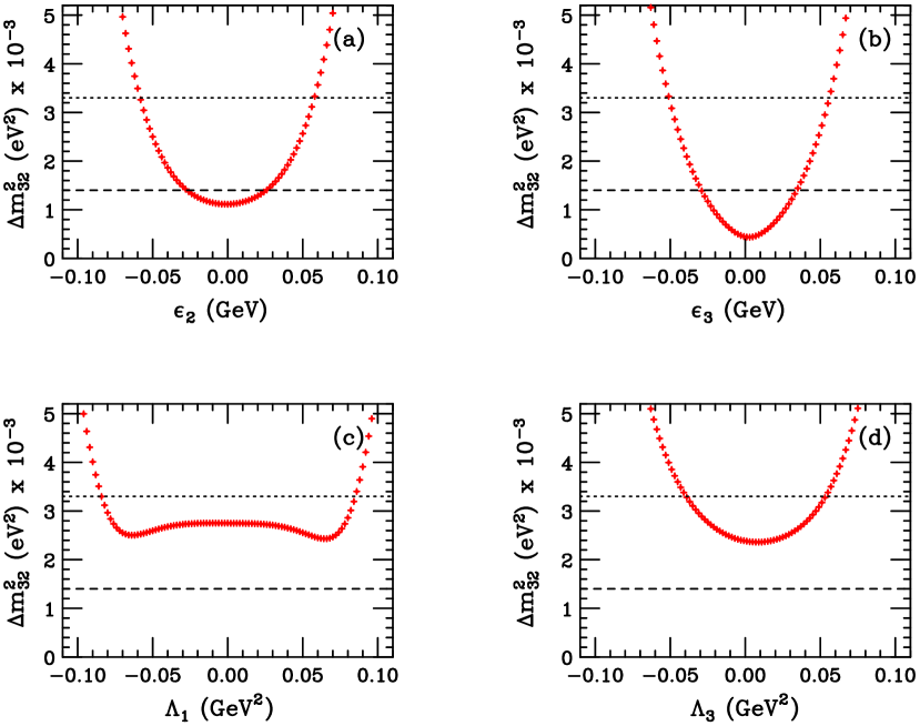
Figure 2: Atmospheric mass squared difference as a function of the four relevant BRpV parameters for the reference scenario: $\epsilon_{2}$, $\epsilon_{3}$, $\Lambda_{1}$, and $\Lambda_{3}$.

In Fig. 2 we have the atmospheric mass squared difference as a function of the four BRpV parameters $\epsilon_{2}$, $\epsilon_{3}$, $\Lambda_{1}$, and $\Lambda_{3}$. The neutrino mass matrix has the texture shown in eq. (14), which implies an atmospheric squared mass difference $\Delta m_{32}^{2}$ given approximately by eq. (24). The parameters $m$ and $a$ in eq. (14) are $m=A\Lambda_{3}^{2}+C\epsilon_{3}^{2}$ and $a=C\epsilon_{2}^{2}/m$, as can be read from eq. (32). The scale $m$ is quadratic in the parameters $\Lambda_{3}$ and $\epsilon_{3}$, since the dependence of $A$ and $C$ on $\Lambda$’s and $\epsilon$’s is weak. The dependence of the atmospheric mass is obtained by replacing these expressions in eq. (24), but when $a\approx 1/2$ the atmospheric scale can be approximated even further obtaining,

$$\Delta m_{32}^{2}\approx{\textstyle{\frac{3}{2}}}\sqrt{5}(A\Lambda_{3}^{2}+C\epsilon_{3}^{2})C\epsilon_{2}^{2}$$ (34)

explaining the quadratic dependency of $\Delta m_{32}^{2}$ on $\epsilon_{2}$, $\epsilon_{3}$ and $\Lambda_{3}$, in frames (2a), (2b), and (2d) respectively, and the mild dependency on $\Lambda_{1}$ (hidden in the neglected terms of order $\lambda^{2}$), as can be observed in frame (2c). The dependence on $\Lambda_{1}$ become strong at high values of this parameter because in that case neglected terms are no longer small.

We note that using the tree level formulae in chapter 2, the atmospheric mass scale would be given by $\Delta m_{32}^{2}\approx(A^{(0)}|\vec{\Lambda}|^{2})^{2}\approx 0.3\times 10^{-3}$ eV², highlighting the inadequacy of the tree level formula. On the contrary, the approximated expression in eq. (34) gives a value $2.8\times 10^{-3}$ eV², which is much closer to the value in eq. (13) found using the complete calculation.

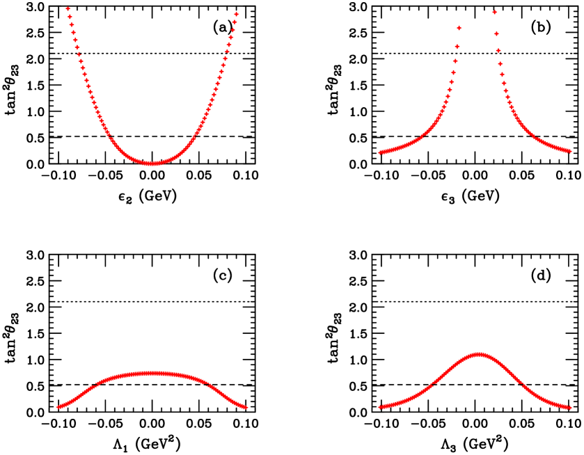
Figure 3: Atmospheric angle as a function of the four relevant BRpV parameters for the reference scenario: $\epsilon_{2}$, $\epsilon_{3}$, $\Lambda_{1}$, and $\Lambda_{3}$.

In Fig. 3 we plot the tangent squared of the atmospheric angle, $\tan^{2}\theta_{23}$. Using eq. (22), or directly from the mass matrix in eq. (32), we find that the atmospheric angle satisfy

$$\tan 2\theta_{23}\approx\frac{2C\epsilon_{2}\epsilon_{3}}{A\Lambda_{3}^{2}+C(\epsilon_{3}^{2}-\epsilon_{2}^{2})}$$ (35)

This relation implies that if $\epsilon_{2}$ approaches zero, the atmospheric angle $\theta_{23}\rightarrow 0$. This behavior is confirmed in frame (3a). On the other hand, if $\epsilon_{3}$ approaches zero then $\theta_{23}\rightarrow\pi/2$ because $C\epsilon_{2}^{2}$ is larger than $A\Lambda_{3}^{2}$, and this explains the divergence of $\tan\theta_{23}$ in frame (3b).

In frame (3c) we see again the mild dependency of the atmospheric parameters on $\Lambda_{2}$, in this case the atmospheric angle. If this parameter becomes very large though, neglected terms of the order $\lambda^{2}$ become important. Finally, the dependency of the atmospheric angle on $\Lambda_{3}$ in frame (3d) can be understood also from eq. (35) since clearly if $|\Lambda_{3}|$ grows then $\tan\theta_{23}$ decreases.

From eq. (9), the tree level atmospheric angle satisfy

$$\tan 2\theta_{23}^{(0)}=\frac{2\Lambda_{2}\Lambda_{3}}{\Lambda_{3}^{2}-\Lambda_{2}^{2}}$$ (36)

and this relation clearly misses all the influence of the one-loop graphs to neutrino mass matrix seen in eq. (35). Numerically, the approximated formula in eq. (35) gives $\tan^{2}\theta_{23}\approx 0.42$, which is close to the value in eq. (13). On the contrary, the tree level formula implies $\tan^{2}\theta_{23}^{(0)}\approx 0$.

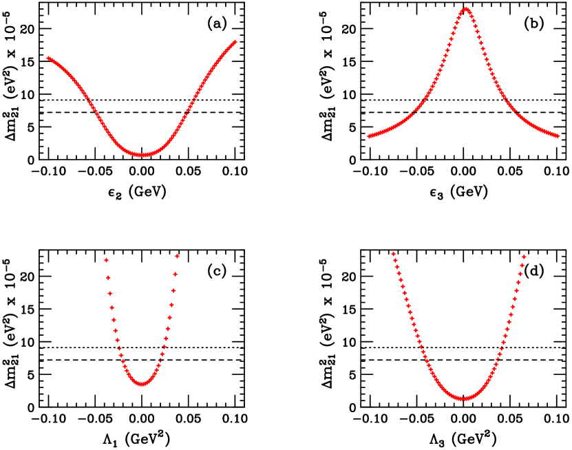
Figure 4: Solar mass squared difference as a function of the four relevant BRpV parameters for the reference scenario: $\epsilon_{2}$, $\epsilon_{3}$, $\Lambda_{1}$, and $\Lambda_{3}$.

In Fig. 4 we plot the solar mass squared difference as a function of the BRpV parameters $\epsilon_{2}$, $\epsilon_{3}$, $\Lambda_{1}$, and $\Lambda_{3}$. In the case of $\Delta m^{2}_{21}$ the neglected terms of order $\lambda^{2}$ in eq. (24) are numerically more important than in the atmospheric case, therefore, predictions based on this approximation are less accurate.

In frame (4a) we see the dependence of the solar mass on $\epsilon_{2}$. This behavior can be understood considering that the parameter $a$ is proportional to $\epsilon_{2}^{2}$, and when this parameter goes to zero, the solar mass difference approaches zero like $a^{2}$, as seen from eq. (24).

In frame (4b) we see how the solar mass difference depends on $\epsilon_{3}$. If $\epsilon_{3}\rightarrow 0$ then the eigenvalue $C\epsilon_{2}^{2}$ decouples and becomes the heaviest neutrino. Of the other two, one neutrino is massless, and the solar mass difference becomes equal to the second neutrino mass squared. A growing $\epsilon_{3}$ will mix the massless neutrino with the heaviest, increasing the lightest neutrino mass, therefore, decreasing the solar mass difference, as observed in frame (4b).

The dependency of the solar mass on $\Lambda_{1}$ and $\Lambda_{3}$ can be understood only if we go beyond the simple approximation in eq. (24). Terms of order $\lambda^{2}$ introduce a dependency on $\Lambda_{1}$ and $\Lambda_{3}$ such that $\lambda$ approaches to zero when these last parameters go to zero, thus explaining the behavior shown in frame (4c) and (4d).

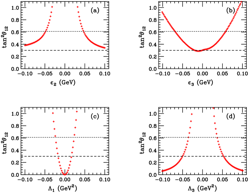
Figure 5: Tangent squared of the solar angle as a function of the four relevant BRpV parameters for the reference scenario: $\epsilon_{2}$, $\epsilon_{3}$, $\Lambda_{1}$, and $\Lambda_{3}$.

In Fig. 5 we have the tangent squared of the solar angle, $\tan^{2}\theta_{12}$, as a function of the BRpV parameters $\epsilon_{2}$, $\epsilon_{3}$, $\Lambda_{1}$, and $\Lambda_{3}$. Working in the texture given in eq. (14), the solar angle according to eq. (22) is approximately given by

$$\tan\theta_{12}=\frac{A\Lambda_{1}^{2}}{m_{\nu_{2}}}\sin\theta_{23}$$ (37)

The dependency on $\Lambda_{1}$ is explicit and comes from the small parameter $\lambda$ in eq. (14). As we know from eqs. (22) and (24), the dependency of $\theta_{23}$ and $m_{\nu_{2}}$ on $\Lambda_{1}$ is weak. The behavior of the solar angle on $\Lambda_{1}$ seen in frame (5c) is thus understood.

The solar angle as a function of $\epsilon_{2}$ can also be easily understood noting that the parameter $a$ is directly proportional to $\epsilon_{2}^{2}$. According to eqs. (17) and (22) the second neutrino mass approaches zero when $a\rightarrow 0$, explaining the divergence shown in frame (5a). Note that $\sin\theta_{23}$ also approaches zero when $\epsilon_{2}\rightarrow 0$, but slower.

The divergence of $\tan\theta_{12}$ when $\Lambda_{3}\rightarrow 0$ is harder to understand from the approximated expression in eq. (37), so we go back to the effective neutrino mass matrix in eq. (32). If $\Lambda_{3}$ approaches zero then the upper-left element of the matrix decouples with a mass $A\Lambda_{1}^{2}$. On the other hand, the lower-right $2\times 2$ sub-matrix has a zero eigenvalue, implying that $\theta_{12}\rightarrow\pi/2$, and therefore explaining the divergence shown in frame (5d).

In Fig. 6 we have chosen the neutrino solution given by the BRpV parameters in eq. (12), and vary the scalar mass $m_{0}$ and the gaugino mass $M_{1/2}$, looking for solutions that satisfy all experimental cuts. In this case, sugra points satisfying the experimental restrictions on the neutrino parameters lie in the shaded region. Solutions are concentrated in a narrow band defined by $M_{1/2}\approx 230-260$ GeV and $m_{0}\approx 0-400$ GeV. We note that in BRpV the LSP need not to be the lightest neutralino, since it is not stable anyway. For this reason, the region close to $m_{0}\approx 0$ is not ruled out.

Smaller values of $M_{1/2}$ are not possible because the atmospheric and solar mass differences become too large. The allowed strip is, thus, limited from below by the curve $\Delta m^{2}_{21}=9.1\times 10^{-5}$ eV². The dependency on $M_{1/2}$ is felt stronger by the tree level contribution to the parameter $A$, given in eq. (30). There we see that $A$ decreases when the gaugino mass $M_{1/2}$ increases, implying that the atmospheric mass decreases with $M_{1/2}$, as seen in eq. (34). In addition, the solar mass difference is proportional to the parameter $m^{2}$, which in turn is proportional to $A$, thus, the solar mass also decreases with the gaugino mass.

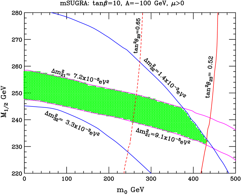
Figure 6: Region of parameter space in the plane $m_{0}-M_{1/2}$ where solutions to neutrino physics passing all the implemented experimental cuts are located. Contours of constant atmospheric mass difference and angle, and solar mass difference are displayed.

Higher values of the scalar mass $m_{0}$ are not allowed because the atmospheric angle becomes too small. The allowed strip is, therefore, limited from the right by the contour $\tan^{2}\theta_{23}=0.52$. We can understand this behavior in the following way: the parameter $C$ decreases with increasing $m_{0}$ due to the Veltman’s functions, and this in turn makes $\tan^{2}\theta_{23}$ to decrease with the scalar mass. High values of the scalar mass are also limited from above because the atmospheric mass becomes too large. This can be explained from eq. (34) considering that the parameter $C$ decreases with increasing $m_{0}$.

Higher values of $M_{1/2}$ are not possible because the solar mass becomes too small, therefore, the allowed stripe is limited from above by the line $\Delta m^{2}_{21}=7.2\times 10^{-5}$ eV². As we already mentioned, the solar mass difference is proportional to the parameter $m^{2}$, which in turn is proportional to $A$, and we already know that $A$ decreases with increasing gaugino mass $M_{1/2}$.

In Fig. 7 we see from another point of view the dependence of the solar and atmospheric mass differences on the scalar mass $m_{0}$, and the gaugino mass $M_{1/2}$. In the plane formed by the atmospheric and solar mass differences we plot four curves defined by a constant value of the scalar mass $m_{0}=100$, 200, 300, and 400 GeV, and vary the gaugino mass in its allowed region, which is indicated in the figure. We keep fixed the values of the BRpV parameters $\epsilon_{i}$ and $\Lambda_{i}$ given eq. (12). The two neutrino mass differences are clearly proportional to each other highlighting their common origin represented by eq. (29), where the parameter $A$ is controlled by tree-level physics and the parameter $C$ is controlled by one-loop physics, and where both are equally important. Fig. 7 can be understood further when seen in relation with Fig. 6.

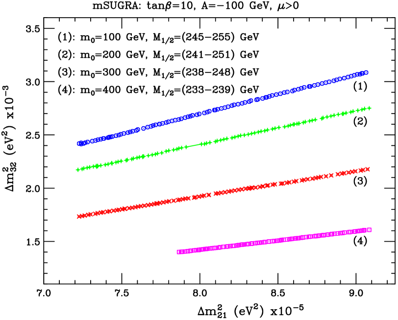
Figure 7: Solutions to neutrino physics in the plane formed with the atmospheric and the solar mass differences. For the three different values of $m_{0}=$100, 150, and 200 GeV, we vary the gaugino mass $M_{1/2}$.

7 Collider Physics

In our model, lepton number and R-Parity are not conserved. One important consequence is that the lightest supersymmetric particle (LSP) is not stable, and will decay into SM particles. Since it is not stable, the LSP needs not to be the lightest neutralino, and whatever it is, its decays can be used to prove the BRpV parameters and the neutrino properties Romao:1999up . In the supergravity benchmark point considered here, the LSP is the lightest neutralino, with a mass $m_{\chi^{0}_{1}}=99$ GeV.

One of the interesting decay modes of the neutralino is $\chi^{0}_{1}\rightarrow W^{\pm}l^{\mp}$, where $l=e,\mu,\tau$. This decay is possible because the neutralino mixes with neutrinos which in turn couple to the pair $Wl$, and also because the charged leptons mix with charginos and they in turn couple to the pair $\chi^{0}_{1}W$. For this reason, the relevant couplings in this decay are in general very dependent on $\epsilon_{i}$ and $\Lambda_{i}$.

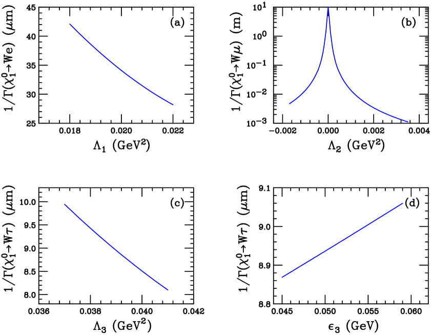
Figure 8: Partial decay width of a neutralino into a $W$ and a lepton, measured in units of distance.

In Fig. 8 we plot the inverse of the partial decay width (multiplied by the velocity of light to convert it into a distance) as a function of the most relevant BRpV parameters. In frame (8a) we see the inverse of $\Gamma(\chi^{0}_{1}\rightarrow We)$ as a function of $\Lambda_{1}$. In fact, for all practical purposes, the decay rate into electrons depends only on $\Lambda_{1}$. Since in first approximation, the coupling is proportional to $\Lambda_{1}$, the inverse of the decay rate behaves like $\Lambda_{1}^{-2}$, and this is seen in the figure. The values of $\Lambda_{1}$ are limited by the solar parameters. The inverse of the partial decay rate $\chi^{0}_{1}\rightarrow We$ is of the order of $30-40\,\mu m$, and it’s an important part of the total decay rate.

In frame (8b) we have the inverse of $\Gamma(\chi^{0}_{1}\rightarrow W\mu)$ as a function of $\Lambda_{2}$, and similarly to the previous case, the decay rate into muons depends practically only on $\Lambda_{2}$. In our reference model in eq. (12) we have $\Lambda_{2}\approx 0$, but values indicated in the figure are also compatible with neutrino physics. The coupling of the neutralino to $W$ and muon is proportional to $\Lambda_{2}$, so the inverse of the decay rate goes like $\Lambda_{2}^{-2}$, and that is observed in frame (8b). Depending on the value of $\Lambda_{2}$, the partial decay length vary from millimeters to more than a hundred meters in the figure. Therefore, this partial decay rate contribute little to the total decay rate of the neutralino.

The inverse of $\Gamma(\chi^{0}_{1}\rightarrow W\tau)$ is plotted in frames (8c) and (8d) as a function of $\Lambda_{3}$ and $\epsilon_{3}$ respectively. The dependence on $\Lambda_{3}$ is stronger and similarly to the previous cases it goes like $\Lambda_{3}^{-2}$. The dependence on $\epsilon_{3}$ is weaker, and the inverse decay rate increases with this parameter. The inverse decay rate is of the order of $8\mu$m, making it the most important contribution to the total decay rate. Neglecting any other decay mode, the total decay rate is near $6\mu$m. The ratios of branching ratios for our benchmark point in eq. (12) are given by

$$\frac{B(\chi^{0}_{1}\rightarrow W\mu)}{B(\chi^{0}_{1}\rightarrow W\tau)}=5.9\times 10^{-5}\,,\qquad\frac{B(\chi^{0}_{1}\rightarrow We)}{B(\chi^{0}_{1}\rightarrow W\tau)}=0.32$$ (38)

We note that if we increase $\Lambda_{2}$ by a factor 4, the first ratio of branching ratios increase to $\sim 10^{-3}$ without changing the other ratio, while still passing all the experimental cuts. In this way, it is clear that by measuring the branching ratios of the neutralinos we get information on the parameters of the model.

The discussion above suggests that the observation of events coming from processes like $pp\rightarrow\chi^{0}_{1}\chi^{0}_{1}\rightarrow WWe\tau$ (at the LHC) or $e^{+}e^{-}\rightarrow\chi^{0}_{1}\chi^{0}_{1}\rightarrow WWe\tau$ (at the NLC) would make possible to measure parameters relevant for neutrino physics.

Figure 9: Feynman diagrams relevant for the production of two neutralinos at the LHC .

We use CompHEP 4.4 comphep to calculate the production cross sections $\sigma(pp\rightarrow\chi^{0}_{1}\chi^{0}_{1})$ (LHC) and $\sigma(e^{+}e^{-}\rightarrow\chi^{0}_{1}\chi^{0}_{1})$ (NLC at $\sqrt{s}=500$ GeV) at leading order. The relevant Feynman diagrams for the LHC are shown in Fig. 9. For the SPS1 mSugra benchmark we obtain:

$$\sigma(pp\rightarrow\chi^{0}_{1}\chi^{0}_{1}) = 9.8\times 10^{-3}\mbox{ pb}$$

$$\sigma(e^{+}e^{-}\rightarrow\chi^{0}_{1}\chi^{0}_{1}) = 0.27\mbox{ pb}$$ (39)

The cross sections of the whole processes were calculated multiplying the production cross sections by the branching ratios $B(\chi^{0}_{1}\rightarrow W^{+}e^{-})$ and $B(\chi^{0}_{1}\rightarrow W^{+}\tau^{-})$. Their values, for the set of parameters we have chosen, are:

$$B(\chi^{0}_{1}\rightarrow W^{+}e^{-}) = 1.9\times 10^{-2}$$

$$B(\chi^{0}_{1}\rightarrow W^{+}\tau^{-}) = 5.9\times 10^{-2}$$ (40)

The complete cross sections are:

$$\sigma(pp\rightarrow\chi^{0}_{1}\chi^{0}_{1}\rightarrow W^{+}W^{+}e^{-}\tau^{-}) = 1.1\times 10^{-5}\mbox{ pb}$$

$$\sigma(e^{+}e^{-}\rightarrow\chi^{0}_{1}\chi^{0}_{1}\rightarrow W^{+}W^{+}e^{-}\tau^{-}) = 3.0\times 10^{-4}\mbox{ pb}$$ (41)

On the other hand, the main source of background comes from the production of four $W$’s with two of them decaying leptonically. We calculated those processes using CompHEP and we found:

$$\sigma(pp\rightarrow WWWW\rightarrow W^{+}W^{+}e^{-}\tau^{-}\bar{\nu_{e}}\bar{\nu_{\tau}}) = 6.5\times 10^{-6}\mbox{ pb}$$

$$\sigma(e^{+}e^{-}\rightarrow WWWW\rightarrow W^{+}W^{+}e^{-}\tau^{-}\bar{\nu_{e}}\bar{\nu_{\tau}}) = 1.6\times 10^{-6}\mbox{ pb}$$ (42)

Assuming a luminosity of $10^{5}$ pb/year at, both, the LHC and the NLC we expect 1 signal event per year at the LHC and 30 signal events per year. Nevertheless we are not interested on the charge of the final leptons, we only require that one lepton belongs to the first family and the other to the third one, so the total number of signal events are obtained by multiplying the above results by four.

We remark that while the background is small in both cases, the number of signal events at the LHC is also small and a more detailed analysis is required. On the other hand the NLC appears as very auspicious environment for studying this model.

8 Conclusions

We have re-examined the possibility of generating neutrino masses and mixing angles in Supergravity with bilinear R-Parity violation. We found solutions with a relatively large value of $\tan\beta$, such that one-loop contributions to the neutralino mass matrix are as important as tree-level contributions. The heaviest neutrino mass is still generated mainly at tree-level, but the other two masses and the three mixing angles are strongly affected by loops. In particular, the tree level approximations for the mixing angles give completely erroneous results.

We concentrate our study on a texture for the neutrino mass matrix which is common among our solutions, and on one particular solution corresponding to this texture. The atmospheric mixing is nearly maximal, and the deviation of the parameter $\tan^{2}\theta_{23}$ from unity is related to the smallness of the ratio between the solar and atmospheric mass scales $\Delta m^{2}_{sol}/\Delta m^{2}_{atm}$. In addition, the solar and reactor angles are both small because of the small parameter $\lambda$, which in turn is small because $\Lambda_{1}/\Lambda_{3}<1$. Nevertheless, the reactor angle is much smaller than the solar angle because the second neutrino mass is much larger than the third one.

We have shown how the neutrino observables depend on the BRpV parameters $\epsilon_{i}$ and $\Lambda_{i}$, and this dependency can be understood in terms of simple approximations in terms of parameters $A$, $B$, and $C$, where all the complication of the one-loop contributions is concentrated. The dependency on $\epsilon_{i}$ and $\Lambda_{i}$ is strong, and it is not clear a priori that a solution is for granted, due to the increasing precision of the measurements of the neutrino observables. It is shown also how these observables depend on the Sugra parameters, namely the universal scalar mass $m_{0}$ and the universal gaugino mass $M_{1/2}$. For the given by the values of $\epsilon_{i}$ and $\Lambda_{i}$, solutions lie in a narrow strip in the plane $m_{0}-M_{1/2}$, where the gaugino mass is strongly restricted by the solar and atmospheric mass scales, and the scalar mass by the atmospheric angle and mass scale.

Finally, we showed how the decay rates of the neutralino depend directly on some of the parameters $\epsilon_{i}$ and $\Lambda_{i}$. In fact $\Gamma(\chi^{0}_{1}\rightarrow We)$ and $\Gamma(\chi^{0}_{1}\rightarrow W\mu)$ depend ${\it only}$ on $\Lambda_{1}$ and $\Lambda_{2}$ respectively, while $\Gamma(\chi^{0}_{1}\rightarrow W\tau)$ depends on both $\Lambda_{3}$ and $\epsilon_{3}$. Measurements on branching ratios of the LSP can therefore give important information on the parameters of the model. We estimated that a few events with $e^{\pm}\tau^{\pm}$ in the final state can be observed at the LHC and about a hundred at the LC, indicating that a measurement of the decay rates is possible at the LC. A more detailed analysis is necessary to estimate the expected precision of these measurements.

References

- [1] Y. Fukuda et al. [Super-Kamiokande Collaboration], Phys. Rev. Lett. 81 (1998) 1562; Q. R. Ahmad et al. [SNO Collaboration], Phys. Rev. Lett. 89 (2002) 011301; K. Eguchi et al. [KamLAND Collaboration], Phys. Rev. Lett. 90 (2003) 021802; Y. Fukuda et al. [Super-Kamiokande Collaboration], Phys. Rev. Lett. 82 (1999) 1810.
- [2] W. Grimus, arXiv:hep-ph/0307149; G. Altarelli and F. Feruglio, arXiv:hep-ph/0306265.
- [3] T. Yanagida, in Proc. of the Workshop on Unified Theory and Baryon Number in the Universe, KEK, 1979; M. Gell-Mann, P. Ramond, and R. Slansky, in Supergravity, Stony Brook, 1979; R.N. Mohapatra and G. Senjanovic, Phys. Rev. Lett. 44, 912 (1980).
- [4] M. Hirsch and J. W. F. Valle, arXiv:hep-ph/0405015.
- [5] G. R. Farrar and P. Fayet, Phys. Lett. B 76 (1978) 575.
- [6] M. Chemtob, arXiv:hep-ph/0406029; R. Barbier et al., arXiv:hep-ph/0406039; B. Allanach et al. [R parity Working Group Collaboration], arXiv:hep-ph/9906224; B. C. Allanach et al., J. Phys. G 24 (1998) 421.
- [7] A. G. Akeroyd, et.al., Nucl. Phys. B 529 (1998) 3; A. Abada, S. Davidson and M. Losada, Phys. Rev. D 65 (2002) 075010; M. A. Diaz, J. Ferrandis, J. C. Romao and J. W. F. Valle, Phys. Lett. B 453 (1999) 263; S. Y. Choi, E. J. Chun, S. K. Kang and J. S. Lee, Phys. Rev. D 60 (1999) 075002; A. G. Akeroyd, M. A. Diaz and J. W. F. Valle, Phys. Lett. B 441 (1998) 224; O. Haug, J. D. Vergados, A. Faessler and S. Kovalenko, Nucl. Phys. B 565 (2000) 38; M. A. Diaz, E. Torrente-Lujan and J. W. F. Valle, Nucl. Phys. B 551 (1999) 78; A. S. Joshipura, R. D. Vaidya and S. K. Vempati, Nucl. Phys. B 639 (2002) 290; S. K. Kang and O. C. W. Kong, Phys. Rev. D 69 (2004) 013004.
- [8] D. F. Carvalho, M. E. Gomez and J. C. Romao, Phys. Rev. D 65 (2002) 093013; M. A. Diaz, J. Ferrandis, J. C. Romao and J. W. F. Valle, Nucl. Phys. B 590 (2000) 3; Y. Grossman and H. E. Haber, Phys. Rev. D 63 (2001) 075011; M. A. Diaz, J. Ferrandis and J. W. F. Valle, Nucl. Phys. B 573 (2000) 75; F. De Campos, et.al., Nucl. Phys. B 623 (2002) 47; M. A. Diaz, R. A. Lineros and M. A. Rivera, Phys. Rev. D 67 (2003) 115004; R. Kitano and K. y. Oda, Phys. Rev. D 61 (2000) 113001; A. G. Akeroyd, E. J. Chun, M. A. Diaz and D. W. Jung, Phys. Lett. B 582 (2004) 64; F. Takayama and M. Yamaguchi, Phys. Lett. B 476 (2000) 116; F. de Campos, et.al., arXiv:hep-ph/0409043.
- [9] M. A. Diaz, In “Valencia 1997, Beyond the standard model: From theory to experiment”, 188-199, arXiv:hep-ph/9802407.
- [10] J. C. Romao, M. A. Diaz, M. Hirsch, W. Porod and J. W. F. Valle, Phys. Rev. D 61 (2000) 071703.
- [11] M. Hirsch, M. A. Diaz, W. Porod, J. C. Romao and J. W. F. Valle, Phys. Rev. D 62 (2000) 113008 [Erratum-ibid. D 65 (2002) 119901].
- [12] P. Nogueira, J. C. Romao and J. W. F. Valle, Phys. Lett. B 251 (1990) 142; M. C. Gonzalez-Garcia and J. W. F. Valle, Nucl. Phys. B 355 (1991) 330; J. C. Romao and J. W. F. Valle, Nucl. Phys. B 381 (1992) 87; M. C. Gonzalez-Garcia, J. C. Romao and J. W. F. Valle, Nucl. Phys. B 391 (1993) 100; J. C. Romao, F. de Campos and J. W. F. Valle, Phys. Lett. B 292 (1992) 329; J. C. Romao, F. de Campos, M. A. Garcia-Jareno, M. B. Magro and J. W. F. Valle, Nucl. Phys. B 482 (1996) 3.
- [13] J. M. Mira, E. Nardi, D. A. Restrepo and J. W. F. Valle, Phys. Lett. B 492 (2000) 81 [arXiv:hep-ph/0007266].
- [14] A. Kogut et al., Astrophys. J. Suppl. 148 (2003) 161.
- [15] H. V. Klapdor-Kleingrothaus, A. Dietz, H. L. Harney and I. V. Krivosheina, Mod. Phys. Lett. A 16 (2001) 2409; C. E. Aalseth et al., Mod. Phys. Lett. A 17 (2002) 1475.
- [16] H. Nunokawa, W. J. C. Teves and R. Zukanovich Funchal, Phys. Lett. B 562 (2003) 28; P. C. de Holanda and A. Y. Smirnov, JCAP 0302 (2003) 001; P. Aliani, V. Antonelli, M. Picariello and E. Torrente-Lujan, Phys. Rev. D 69 (2004) 013005; J. N. Bahcall, M. C. Gonzalez-Garcia and C. Pena-Garay, JHEP 0302 (2003) 009; G. L. Fogli, E. Lisi, A. Marrone, D. Montanino, A. Palazzo and A. M. Rotunno, Phys. Rev. D 67 (2003) 073002; V. Barger and D. Marfatia, Phys. Lett. B 555 (2003) 144; A. Bandyopadhyay, S. Choubey, R. Gandhi, S. Goswami and D. P. Roy, Phys. Lett. B 559 (2003) 121.
- [17] M. Maltoni, T. Schwetz, M. A. Tortola and J. W. F. Valle, arXiv:hep-ph/0405172.
- [18] A. Djouadi, J. L. Kneur and G. Moultaka, arXiv:hep-ph/0211331.
- [19] N. Ghodbane and H. U. Martyn, arXiv:hep-ph/0201233.
- [20] H. V. Klapdor-Kleingrothaus, arXiv:hep-ph/0307330.
- [21] M. A. Diaz, M. Hirsch, W. Porod, J. C. Romao and J. W. F. Valle, Phys. Rev. D 68 (2003) 013009 [arXiv:hep-ph/0302021].
- [22] A. Y. Smirnov, arXiv:hep-ph/0402264; R. N. Mohapatra, arXiv:hep-ph/0402035.
- [23] M. Hirsch and W. Porod, Phys. Rev. D 68 (2003) 115007; A. Bartl, M. Hirsch, T. Kernreiter, W. Porod and J. W. F. Valle, JHEP 0311 (2003) 005; M. B. Magro, F. de Campos, O. J. P. Eboli, W. Porod, D. Restrepo and J. W. F. Valle, JHEP 0309 (2003) 071; D. Restrepo, W. Porod and J. W. F. Valle, Phys. Rev. D 64 (2001) 055011; D. W. Jung, S. K. Kang, J. D. Park and E. J. Chun, arXiv:hep-ph/0407106; Phys. Rev. D 66 (2002) 073003; M. A. Diaz, D. A. Restrepo and J. W. F. Valle, Nucl. Phys. B 583 (2000) 182; A. Belyaev, M. H. Genest, C. Leroy and R. R. Mehdiyev, arXiv:hep-ph/0401065; D. Aristizabal Sierra, M. Hirsch and W. Porod, arXiv:hep-ph/0409241.
-
[24]
CompHEP - a package for evaluation of Feynman diagrams and integration
over multi-particle phase space. User’s manual for version 3.3,
hep-ph/9908288
COMPHEP 4.4 - AUTOMATIC COMPUTATIONS FROM LAGRANGIANS TO EVENTS. E.Boos, V.Bunichev, M.Dubinin, L.Dudko, V.Ilyin, A.Kryukov, V.Edneral, V.Savrin, A.Semenov, A.Sherstnev. Mar 2004. 10pp. e-Print Archive: hep-ph/0403113
Home page: http://theory.sinp.msu.ru/comphep