Abstract

We discuss the possibilities of high precision measurement of the solar neutrino mixing angle $\theta_{\odot}\equiv\theta_{12}$ in solar and reactor neutrino experiments. The improvements in the determination of $\sin^{2}\theta_{12}$, which can be achieved with the expected increase of statistics and reduction of systematic errors in the currently operating solar and KamLAND experiments, are summarised. The potential of LowNu $\nu-e$ elastic scattering experiment, designed to measure the $pp$ solar neutrino flux, for high precision determination of $\sin^{2}\theta_{12}$, is investigated in detail. The accuracy in the measurement of $\sin^{2}\theta_{12}$, which can be achieved in a reactor experiment with a baseline $L\sim(50-70)$ km, corresponding to a Survival Probability MINimum (SPMIN), is thoroughly studied. We include the effect of the uncertainty in the value of $\sin^{2}\theta_{13}$ in the analyses. A LowNu measurement of the $pp$ neutrino flux with a 1% error would allow to determine $\sin^{2}\theta_{12}$ with an error of 14% (17%) at 3$\sigma$ from a two-generation (three-generation) analysis. The same parameter $\sin^{2}\theta_{12}$ can be measured with an uncertainty of 2% (6%) at 1$\sigma$ (3$\sigma$) in a reactor experiment with $L\sim 60$ km, statistics of $\sim$60 GWkTy and systematic error of 2%. For the same statistics, the increase of the systematic error from 2% to 5% leads to an increase in the uncertainty in $\sin^{2}\theta_{12}$ from 6% to 9% at 3$\sigma$. The inclusion of the $\sin^{2}\theta_{13}$ uncertainty in the analysis changes the error on $\sin^{2}\theta_{12}$ to 3% (9%). The effect of $\sin^{2}\theta_{13}$ uncertainty on the $\sin^{2}\theta_{12}$ measurement in both types of experiments is considerably smaller than naively expected.

1 Introduction

There has been a remarkable progress in the studies of neutrino oscillations in the last several years. The experiments with solar, atmospheric and reactor neutrinos [1, 2, 3, 4, 5, 6, 7] have provided compelling evidences for the existence of neutrino oscillations driven by non–zero neutrino masses and neutrino mixing. Evidences for oscillations of neutrinos were obtained also in the first long baseline accelerator neutrino experiment K2K [8].

The recent Super-Kamiokande data on the $L/E$-dependence of multi-GeV $\mu$-like atmospheric neutrino events [6], $L$ and $E$ being the distance traveled by neutrinos and the neutrino energy, and the new more precise spectrum data of KamLAND and K2K experiments [9, 10], are the latest significant contributions to this progress. For the first time the data exhibit directly the effects of the oscillatory dependence on $L/E$ and $E$ of the probabilities of $\nu$-oscillations in vacuum [11]. We begin to “see” the oscillations of neutrinos. As a result of these magnificent developments, the oscillations of solar $\nu_{e}$, atmospheric $\nu_{\mu}$ and $\bar{\nu}_{\mu}$, accelerator $\nu_{\mu}$ (at $L\sim$250 km) and reactor $\bar{\nu}_{e}$ (at $L\sim$180 km), driven by nonzero $\nu$-masses and $\nu$-mixing, can be considered as practically established.

The SK atmospheric neutrino and K2K data are best described in terms of dominant 2-neutrino $\nu_{\mu}\rightarrow\nu_{\tau}$ ($\bar{\nu}_{\mu}\rightarrow\bar{\nu}_{\tau}$) vacuum oscillations. The best fit values and the 99.73% C.L. allowed ranges of the atmospheric neutrino oscillation parameters $|\Delta m^{2}_{\rm A}|=|\Delta m^{2}_{31}|$ and $\theta_{\rm A}\equiv\theta_{23}$ read [6]: $|\Delta m^{2}_{31}|=2.1\times 10^{-3}~{}{\rm eV^{2}}$,  $\sin^{2}2\theta_{23}=1.0$, $|\Delta m^{2}_{31}|=(1.3-4.2)\times 10^{-3}~{}{\rm eV^{2}}$, $\sin^{2}2\theta_{23}\geq 0.85$. The sign of $\Delta m^{2}_{31}$ and of $\cos 2\theta_{23}$, if $\sin^{2}2\theta_{23}\neq 1.0$, cannot be determined using the existing data.

The combined 2-neutrino oscillation analysis of the solar neutrino and the new KamLAND 766.3 Ty spectrum data shows [9, 12, 13] that the solar neutrino oscillation parameters lie in the low-LMA region : $\Delta m^{2}_{\odot}\equiv\Delta m^{2}_{21}=(7.9^{+0.6}_{-0.5})\times 10^{-5}~{}{\rm eV^{2}}$, $\tan^{2}\theta_{\odot}\equiv\tan^{2}\theta_{12}=(0.40^{+0.09}_{-0.07})$ [9]. The high-LMA solution is excluded at more than 3$\sigma$. The value of $\Delta m^{2}_{21}$ is determined with a remarkably high precision of 12% at 3$\sigma$. Maximal solar neutrino mixing is ruled out at $\sim 6\sigma$.

The solar and atmospheric neutrino, and KamLAND and K2K neutrino oscillation data require the existence of three-neutrino mixing in the weak charged lepton current. In this case the neutrino mixing is characterised by one additional mixing angle $\theta_{13}$ – the only small mixing angle in the PMNS matrix. Three-neutrino oscillation analyses of the solar, atmospheric and reactor neutrino data show that $\sin^{2}\theta_{13}<0.05$ [12, 13] .

Understanding the origin of the patterns of solar and atmospheric neutrino mixing and of $\Delta m^{2}_{21}$ and $\Delta m^{2}_{31}$, suggested by the data, is one of the central problems in neutrino physics today. A pre-requisite for any progress in our understanding of neutrino mixing is the knowledge of the precise values of solar and atmospheric neutrino oscillation parameters, $\theta_{12}$, $\Delta m^{2}_{21}$, and $\theta_{23}$, $\Delta m^{2}_{31}$ and of $\theta_{13}$. In the present article we discuss the possibilities of high precision measurement of the solar neutrino mixing angle $\theta_{12}$ in solar and reactor neutrino experiments.

The solar neutrino mixing parameter $\sin^{2}\theta_{12}$ is determined by the current KamLAND and solar neutrino data with a relatively large uncertainty of 24% at 3$\sigma$. In the future, more precise spectrum data from the KamLAND experiment can lead to even more accurate determination of the value of $\Delta m^{2}_{21}$. However, these data will not provide a considerably more precise measurement of $\sin^{2}\theta_{12}$ owing to the fact that the baseline of the KamLAND experiment effectively corresponds to a $\bar{\nu}_{e}$ Survival Probability MAXimum (SPMAX) [16, 17]. The analysis of the global solar neutrino data taking into account a possible reduction of the errors in the data from the phase-III of the SNO experiment shows that the uncertainty in the value of $\sin^{2}\theta_{12}$ would still remain well above 15% at $3\sigma$ [18].

We begin by summarising the results on $\sin^{2}\theta_{12}$, obtained using the current global solar and reactor neutrino oscillation data (section 2). We consider the improvements in the determination of $\sin^{2}\theta_{12}$, which can be achieved with the expected increase of statistics and reduction of systematic errors in the experiments which are currently operating. In particular, the effect of KamLAND data, corresponding to a statistics of 3 kTy, as well as of the data of phase-III of SNO experiment, are analysed.

We turn next to future experiments. We discuss first (in section 3) the possibility of high precision determination of $\sin^{2}\theta_{12}$ in a LowNu solar neutrino experiment, designed to measure the $\sim$MeV and sub-MeV components of the solar neutrino flux: $pp$, $pep$, $CNO$, ${}^{7}{Be}$. It is usually suggested that the LowNu experiments can provide one of the most precise measurements of the solar neutrino mixing angle [19, 20, 21]. Detailed analysis was carried out in [22] and it was concluded that a future $pp$ experiment should have accuracy better than 3% in order to improve on the knowledge of $\tan^{2}\theta_{12}$.

We consider a generic $\nu-e$ scattering experiment measuring the $pp$ neutrino flux and perform a detailed quantitative analysis of the precision with which $\sin^{2}\theta_{12}$ can be determined in such an experiment. We examine the effect of including different representative values of the $pp$ neutrino induced event rate in the $\chi^{2}$ analysis of the global solar neutrino data. Three values (0.68, 0.72, 0.77) of the (normalized) event rate from the currently allowed 3$\sigma$ range are considered. The error in the measured rate is varied from 1% to 5%. We investigate how much the accuracy on $\sin^{2}\theta_{12}$ improves by adding the $pp$ flux data in the analysis. The dependence of the sensitivity to $\sin^{2}\theta_{12}$ on the central value of the measured $pp$ flux as well as on the measurement errors is studied. We compare the precision in $\sin^{2}\theta_{12}$ expected with assumed data on $pp$ neutrinos included in the analysis, with the sensitivity that can be achieved using prospective results from phase-III of SNO experiment and 3 kTy KamLAND data, and comment on the minimum error required in the LowNu $pp$ experiments to improve the precision of $\sin^{2}\theta_{12}$ measurement. The impact of the uncertainty due to $\theta_{13}$ on the allowed ranges of $\sin^{2}\theta_{12}$ is studied as well.

In the section 4 we analyse in detail the possibility of a high precision determination of $\sin^{2}\theta_{12}$ in a reactor experiment with a baseline of $L\sim(50-70)$ km, corresponding to a $\bar{\nu}_{e}$ Survival Probability MINimum (SPMIN). That such an experiment can provide the highest precision in the measurement of $\sin^{2}\theta_{12}$ was pointed out first in [16]. A rather detailed study of the precision in $\sin^{2}\theta_{12}$, which might be achieved in an SPMIN experiment with the flux of $\bar{\nu}_{e}$ from the Kashiwazaki reactor complex in Japan and $L=54$ km, was performed recently in [23] . We consider a generic SPMIN reactor experiment with a KamLAND-type detector. We investigate the dependence of the precision on $\sin^{2}\theta_{12}$ which can be achieved in such an experiment on the baseline, statistics and systematic errors. More specifically, the spectrum data is simulated for four different true values of $\Delta m^{2}_{21}$ and for each of these values the optimal baseline at which the most precise measurement of $\sin^{2}\theta_{12}$ could be performed is determined. We show, in particular, that an independent determination of $\Delta m^{2}_{21}$ with sufficiently high accuracy would allow $\sin^{2}\theta_{12}$ to be measured with the highest precision over a relatively wide range of baselines. The effect of $\sin^{2}\theta_{13}$ uncertainty on the $\sin^{2}\theta_{12}$ determination is investigated in detail.

The results of the present study are summarised in section 5.

2 Measuring $\sin^{2}\theta_{12}$ in Existing Experiments

In this section we review the precision of $\Delta m_{21}^{2}$  and $\sin^{2}\theta_{12}$ determination from the existing solar neutrino and KamLAND data from two-neutrino oscillation analysis. We also discuss possible improvements in the precision that can be achieved in the currently running experiments.

2.1 Current Solar and Reactor Neutrino Data on $\sin^{2}\theta_{12}$

In the present global solar neutrino and KamLAND data analysis we include

• data from the radiochemical experiments, Cl [1] and Ga (Gallex, SAGE and GNO combined) [2],

• the 1496 day 44 bin Zenith angle spectrum data from SK [3],

• the 34 bin combined CC, NC and Electron Scattering (ES) energy spectrum data from the phase I ( pure $D_{2}O$ phase) of SNO [4],

• the data on CC, NC and ES total observed rates from the phase II (salt phase) of SNO experiment [5].

The ${}^{8}B$ flux normalization factor $f_{B}$ is left to vary freely in the analysis, while for the $pp$, $pep$, ${}^{7}Be$, $CNO$, and $hep$ fluxes the predictions and uncertainties from the recent standard solar model (SSM) [24] (BP04) are used. We skip the details of the $\chi^{2}-$ analysis, which can be found in [25, 26, 27].

We include the 766.3 Ty KamLAND data in the global analysis. For treatment of the latest KamLAND data in the combined analysis we refer the reader to [12], while details regarding the future-projected analysis with simulated KamLAND data are given in [28]. The best-fit in the combined analysis of solar and KamLAND data is obtained for [12]

• $\Delta m^{2}_{21}=8.4\times 10^{-5}$ eV²,    $\sin^{2}\theta_{12}=0.28$,    $\mathrm{f}_{B}$ = 0.88

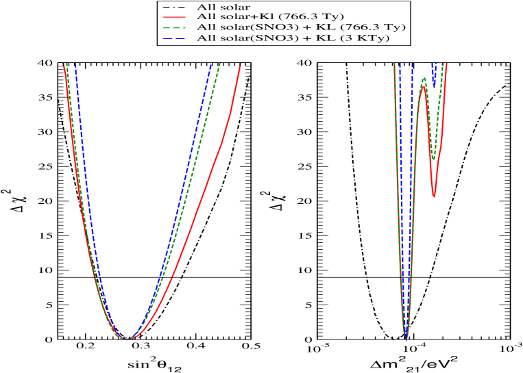
Figure 1: $\Delta\chi^{2}$ as a function of $\sin^{2}\theta_{12}$ (left panel) and of $\Delta m_{21}^{2}$  (right panel). The curves shown are obtained from global analysis of the current solar neutrino data (black dot-dashed line), current solar + KamLAND data (red solid line), solar neutrino data with projected SNO-III errors + current KamLAND data (green short dashed line) and the solar neutrino data with projected SNO-III errors + prospective 3 kTy KamLAND data (blue long dashed line). The horizontal lines indicate the 3$\sigma$ limit ($\Delta\chi^{2}=9$) for 1 parameter fit.

In Fig. 1 we plot $\Delta\chi^{2}=\chi^{2}-\chi^{2}_{min}$ as a function of $\Delta m_{21}^{2}$  (right panel) and $\sin^{2}\theta_{12}$ (left panel), for a two-neutrino oscillation fit of the global solar neutrino + KamLAND data. The parameters not given in each of the two panels are allowed to vary freely. From this figure one can easily read off the allowed ranges of the displayed parameter at various confidence levels. The horizontal line shows the 3$\sigma$ limit corresponding to $\Delta\chi^{2}=9$ for a 1 parameter fit. In Table 1 we present the current 3$\sigma$ allowed ranges of $\Delta m_{21}^{2}$  and $\sin^{2}\theta_{12}$ obtained from Fig. 1. We also give the spread in these parameters which is defined as

$${\rm spread}=\frac{prm_{max}-prm_{min}}{prm_{max}+prm_{min}}\times 100$$ (1)

where ${prm}$ is either $\Delta m_{21}^{2}$ or $\sin^{2}\theta_{12}$. Table 1 and Fig. 1 demonstrate clearly that the KamLAND  experiment has remarkable sensitivity to $\Delta m_{21}^{2}$ . The inclusion of KamLAND data with increasing statistics in the analysis progressively reduces the spread in $\Delta m_{21}^{2}$ , and with the latest data the 3$\sigma$ spread is $\sim$ 12%. This demonstrates, in particular, the extraordinary precision that has already been achieved in the determination of $\Delta m^{2}_{21}$. On the other hand, the spread in $\sin^{2}\theta_{12}$ is seen to be controlled mainly by the solar neutrino data and does not show any marked reduction with the inclusion of the KamLAND data in the analysis. Using the global solar neutrino and KamLAND data allows to determine $\sin^{2}\theta_{12}$ with an error of 24% at 3$\sigma$.

2.2 Prospective KamLAND and SNO Data and $\sin^{2}\theta_{12}$

We will analyze next the expected impact of future data from KamLAND and SNO experiments on the $\Delta m^{2}_{21}$ and $\sin^{2}\theta_{12}$ determination.

The SNO experiment is sensitive to the flux of ${}^{8}B$ neutrinos with energy $E\ \raisebox{-1.72218pt}{\hbox to0.0pt{$\sim$\hss}}\raisebox{1.72218pt}{$>$}\ 5$ MeV. For the oscillation parameters in the low-LMA region, the ${}^{8}B$ neutrino survival probability of interest is given approximately by (MSW adiabatic transition probability):

$$P_{ee}({\mbox{${}^{8}{B}~{}$}})\approx\sin^{2}\mbox{$\theta_{12}$~{}}.$$ (2)

The CC/NC ratio measured in SNO determines $P_{ee}$ independently of the ${}^{8}B$ neutrino flux normalization. Thus, it can give a direct measure of $\sin^{2}\theta_{12}$. Reducing the errors ($\Delta({R_{CC}/R_{NC}}$) in the measured CC and NC event rates in SNO, $R_{CC}$ and $R_{NC}$, can improve the precision of determination of this parameter since

$$\Delta({\sin^{2}\theta_{12}})=\Delta({R_{CC}/R_{NC}}).$$ (3)

The oscillations of reactor $\bar{\nu}_{e}$ detected in KamLAND experiment are practically not affected by Earth matter effects and the corresponding $\bar{\nu}_{e}$ survival probability has the form

$$P_{\bar{e}\bar{e}}^{KL}\approx 1-\sin^{2}2\theta_{12}\sin^{2}\left(\frac{\mbox{$\Delta m_{21}^{2}$~{}}L}{4E}\right).$$ (4)

The average energy and baseline for KamLAND correspond to $\sin^{2}(\mbox{$\Delta m_{21}^{2}$~{}}L/4E)\approx 0$, i.e., to a Survival Probability MAXimum (SPMAX). As a consequence, the coefficient of the $\sin^{2}2\theta_{12}$ term in $P_{\bar{e}{e}}^{KL}$ is relatively small, weakening the sensitivity of KamLAND to $\theta_{12}$. As was shown in [16], the most precise measurement of $\sin^{2}\theta_{12}$ can be performed in a reactor experiment with a baseline tuned to a Survival Probability MINimum (SPMIN), i.e., to $\sin^{2}(\mbox{$\Delta m_{21}^{2}$~{}}L/4E)\approx 1$. We will discuss the sensitivity to $\sin^{2}\theta_{12}$, which can be achieved in such an experiment, in section 4.

In phase-III of the SNO experiment, the NC events will be observed directly (and independently from the CC events) using ${}^{3}He$ proportional counters. This will help to increase the NC statistics and reduce the systematic errors in the NC data. In addition, the correlations between the errors in the measured CC and NC event rates will be absent. The total projected error in the measured NC event rate in phase-III of SNO experiment is $\sim 6\%$ [29]. We incorporate this in our analysis instead of the present error in $R_{NC}$ of 9%. For the CC event rate $R_{CC}$ measured at SNO we assume a somewhat reduced total error of 5% (the current error in $R_{CC}$ is approximately 6% [14]). We assume also that the central values of the measured CC and NC even rates will remain unchanged. The results of our analysis are shown in Fig. 1. The short dashed lines in Fig. 1 display the behavior of $\Delta\chi^{2}$ with anticipated SNO phase-III results and the reduced projected errors added to the global solar neutrino and KamLAND 766.3 Ty spectrum data. The figure shows that with the inclusion of the SNO phase-III prospective results, the allowed range of $\Delta m_{21}^{2}$  in the low-LMA region remains unchanged: it is determined principally by the KamLAND data. However, the higher $\Delta m_{21}^{2}$  regions get more disfavored as the reduced errors in $R_{CC}$ and $R_{NC}$ lead to a stronger rejection of larger values of $R_{CC}/R_{NC}$ [30]. The figure also shows that the allowed range of $\sin^{2}\theta_{12}$ gets further constrained from above. From Table 1 we see that the 3$\sigma$ spread of $\sin^{2}\theta_{12}$ becomes 21% with the inclusion of projected SNO phase-III data in the presently existing set of data.

We also studied the effect of increased statistics of KamLAND experiment on the $\sin^{2}\theta_{12}$ and $\Delta m^{2}_{21}$ determination. To this end, we include 3 kTy KamLAND spectrum data, simulated at $\mbox{$\Delta m_{21}^{2}$~{}}=8.3\times 10^{-5}$ eV², in our analysis with projected SNO phase-III data. We use a systematic error of 5% for KamLAND since the KamLAND systematic error is expected to diminish after the planned fiducial volume calibration and re-evaluation of the uncertainties in the power of the relevant nuclear stations. If the real KamLAND spectrum data conforms to this projected spectrum, the allowed range of $\Delta m_{21}^{2}$  would be further constrained, allowing the determination of $\Delta m_{21}^{2}$  with an accuracy of about 5%. The higher $\Delta m_{21}^{2}$ regions would be disfavored even stronger. The uncertainty in the value of $\sin^{2}\theta_{12}$ would be smaller and the 3$\sigma$ spread, as seen from Table 1, could be 18%. Clearly, the uncertainty in $\sin^{2}\theta_{12}$ cannot be reduced to 15% or less (at 3$\sigma$) by future data from the currently operating solar and reactor neutrino experiments

Data set	(3$\sigma$)Range of	(3$\sigma$)spread in	(3$\sigma$) Range of	(3$\sigma$) spread in
used	$\Delta m^{2}_{21}$ eV2	$\Delta m^{2}_{21}$	$\sin^{2}\theta_{12}$	$\sin^{2}\theta_{12}$
only sol	3.3 - 15.3	65%	$0.22-0.38$	27%
sol+ 766.3 Ty KL	7.4 - 9.5	12%	$0.22-0.36$	24%
sol(+SNO3) + 766.3 Ty KL	7.4 -9.5	12%	0.22 - 0.34	21%
sol(+SNO3)+3KTy KL	7.7 -8.9	7%	0.23 - 0.33	18%

Table 1: The 3$\sigma$ allowed ranges and spread (in per cent) of $\Delta m^{2}_{21}$ and $\sin^{2}\theta_{12}$ obtained from 1 parameter fits.

3 Determining $\theta_{12}$ from Measurement of the $pp$ Solar Neutrino Flux

The $pp$ fusion reaction is the main contributor to the observed solar luminosity and the corresponding $pp$ neutrinos constitute the largest and dominant component of the solar neutrino flux. The SSM uncertainty in the predicted solar neutrino fluxes is the least for the $pp$ neutrinos ($\sim$1%) [24]. So far only the Ga experiments have provided information on the $pp$ neutrino flux because of their low energy threshold of 0.23 MeV. Sub-MeV solar neutrino experiments (LowNu experiments) are being planned for measuring the flux of $pp$ neutrinos using either charged current reactions (LENS, MOON, SIREN) or $\nu-e^{-}$ elastic scattering (XMASS, CLEAN, HERON, MUNU, GENIUS) [19, 20, 21]. Since according to the SSM, most of the energy released by the Sun ($\sim$99%) is generated in the $pp-$cycle of reactions in which also the $pp$ neutrinos are produced, a precise determination of the $pp$ neutrino flux would lead to a better understanding of the solar energetics and, more generally, of the physics of the Sun. It has also been realized that high precision measurement of the $pp$ neutrino flux can be instrumental for more accurate determination of the solar neutrino mixing parameter, which, as we have seen in the preceding section, will not be determined with an uncertainty smaller than $\sim$18% (at 3$\sigma$) by the currently operating experiments.

Since the $pp$ neutrino energy spectrum extends upto 0.42 MeV only, for $\Delta m^{2}_{21}$ in the LMA region, the $pp$ neutrino oscillations are practically not affected by matter effects in the Sun or the Earth. Thus, to a good approximation, the $pp$ neutrino oscillations are described by the $\nu_{e}$ survival probability in the case of oscillations in vacuum, in which the oscillating term is strongly suppressed by the averaging over the region of neutrino production in the Sun [31]:

$$P_{ee}^{2\nu}(pp)\cong 1-\frac{1}{2}\sin^{2}2\theta_{12}.$$ (5)

The normalised event rate for a $\nu-e$ scattering (ES) and charged current (CC) experiments measuring the $pp$ neutrino flux is given respectively by

$$R_{pp} = \langle{P_{ee}^{2\nu}(pp)}\rangle+r_{pp}(1-\langle{P_{ee}^{2\nu}(pp)}\rangle)~{}~{}{\mathrm{for~{}~{}ES~{}~{}experiments}},$$ (6)

$$R_{pp} = \langle{P_{ee}^{2\nu}(pp)}\rangle~{}~{}~{}~{}~{}~{}~{}~{}~{}~{}~{}~{}~{}~{}~{}~{}~{}~{}~{}~{}~{}~{}~{}~{}{\mathrm{for~{}~{}CC~{}~{}experiments}},,$$ (7)

where $r_{pp}=\int f_{pp}(E)\sigma(\nu_{\mu(\tau)}e^{-})dE/\int f_{pp}(E)\sigma(\nu_{e}e^{-})dE\approx 0.3$ where $f_{pp}(E)$ is the pp-neutrino flux, $\sigma(\nu_{\mu(\tau)}e^{-})$ and $\sigma(\nu_{e}e^{-})$ are the $\nu_{\mu(\tau)}-e^{-}$ and $\nu_{e}-e^{-}$ eleastic scattering cross sections and $\langle..\rangle$ denotes averaged probabilites.

For an ES experiment, the second term in eq. (6) represents the NC contribution. Since the pp neutrino survival probability is largely independent of energy one can use eq. 5 for the averaged probabilites . Using eqs. (5) - (7), one finds for the uncertainty in $\sin^{2}\theta_{12}$ determination:

$$\Delta({\sin^{2}\theta_{12}})^{CC}_{pp}\sim\frac{\Delta{R_{pp}}}{2\cos 2\theta_{12}}~{}~{}{\mathrm{for~{}~{}CC~{}~{}experiments}}$$ (8)

$$\Delta({\sin^{2}\theta_{12}})^{ES}_{pp}\sim\frac{\Delta{R_{pp}}}{2\cos 2\theta_{12}}\frac{1}{1-r_{pp}}~{}~{}{\mathrm{for~{}~{}ES~{}~{}experiments}}$$ (9)

where $\Delta{R_{pp}}$ is the error in the measured value of $R_{pp}$. A comparison of eq. (8) with eq. (3) shows that for the same value of $\Delta{R_{pp}}$ and of the error in the CC to NC event rate ratio measured by SNO, $\Delta({R_{CC}/R_{NC}})$, the $pp$ neutrino experiments of the CC type can provide a more precise measurement of $\sin^{2}\theta_{12}$ only if $\cos 2\theta_{12}>0.5$ ($\sin^{2}\theta_{12}<0.25$). Similarly, it follows from eq. (9) and eq. (3) that for $\Delta{R_{pp}}\cong\Delta({R_{CC}/R_{NC}})$, the ES $pp$ experiment could provide a more precise determination of $\sin^{2}\theta_{12}$ only if the true value of $\cos 2\theta_{12}>0.71$ ($\sin^{2}\theta_{12}<0.14$). Since the currently allowed 3$\sigma$ range of $\sin^{2}\theta_{12}$ is $\sin^{2}\theta_{12}=(0.22-0.38)$, for almost all of the allowed values of $\sin^{2}\theta_{12}$, SNO will have a better sensitivity to $\sin^{2}\theta_{12}$ than a LowNu $pp$ experiment measuring the $pp$ neutrino flux with the same experimental error as the error in the SNO data on the ratio $R_{CC}/R_{NC}$.

In order to improve the accuracy of $\sin^{2}\theta_{12}$ determination after the SNO phase-III results will be available, the total experimental error in the measured event rate in the $pp$ experiments has to be sufficiently small, which requires high statistics and well understood systematics. In the present section we will quantify these statements by incorporating hypothetical data on the $pp$ neutrino flux in our analysis. We consider a generic $pp$ neutrino ES experiment and consider some illustrative sample rates from the currently predicted range. We give quantitative estimate of the sensitivity to $\sin^{2}\theta_{12}$ expected to be achieved in i) a $pp$ experiment, and ii) combining the prospective data from a $pp$ experiment with the global solar and reactor neutrino data. In particular, we estimate the maximal error in a $pp$ flux measurement, for which the uncertainty in the determined value of $\sin^{2}\theta_{12}$ would be smaller than that expected after the inclusion of the SNO phase-III results. We use in this analysis the $pp$ neutrino flux and its 1% uncertainty predicted by the BP04 SSM [24]. The 1% error due to SSM uncertainties is added to the experimental errors in the $pp$ flux determination.

3.1 Two Generation Analysis

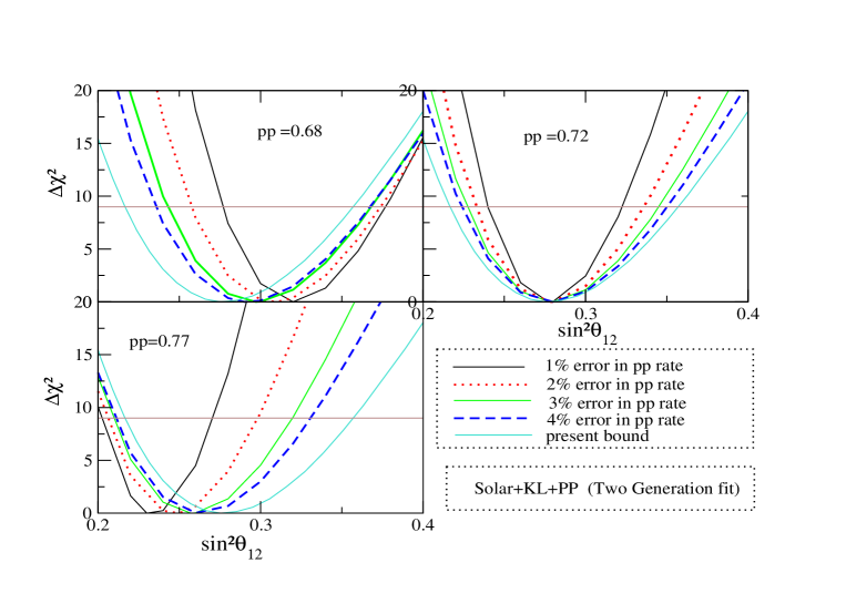
Figure 2: $\Delta\chi^{2}$ as a function of $\sin^{2}\theta_{12}$. The results shown are obtained in a two-neutrino oscillation analysis of the global solar neutrino and KamLAND 766.3 Ty spectrum data and simulated data from a LowNu $pp$ neutrino experiment. The three panels correspond to three illustrative values of the event rate due to $pp$ neutrinos in the LowNu experiment (“$pp$ rate”), normalized to the rate predicted by the BP04 SSM. In each case results for four different assumed values of the error in the measured $pp$ rate are shown. We also show the curve obtained in global analysis of the current solar and reactor neutrino data. The horizontal line indicates the 3$\sigma$ limit ($\Delta\chi^{2}=9$) for 1 parameter fit.

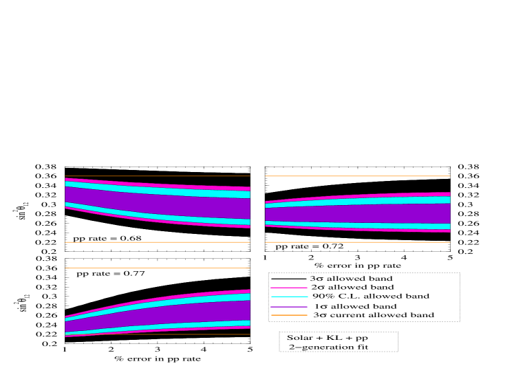
Figure 3: The 1$\sigma$ (68.27% C.L.), 1.64$\sigma$ (90% C.L.), 2$\sigma$ (95.45% C.L.) and 3$\sigma$ (99.73% C.L.) allowed range of $\sin^{2}\theta_{12}$ as a continuous function of the error in the $pp$ rate for three assumed mean values of the measured $pp$ rate. Shown is also the current 3$\sigma$ allowed range of $\sin^{2}\theta_{12}$.

We consider a generic $\nu-e$ scattering experiment which can measure the $pp$ neutrino flux. The experiment is assumed to have $e^{-}$ kinetic energy threshold of 50 keV. We suppose that the BP04 SSM predicts correctly the $pp$ flux. The predicted event rate (“$pp$ rate”) in such an experiment for the best fit values of the oscillation parameters, normalized to the rate predicted by the BP04 model in the absence of neutrino oscillations, is 0.71; the predicted 3$\sigma$ range for the normalized $pp$ rate is $0.67-0.76$ [12]. We will consider three illustrative values of the normalized $pp$ rate, 0.68, 0.72 and 0.77, and vary the experimental error in the measured $pp$ rate from 1% to 5%. The estimated theoretical uncertainties due to the SSM and their correlations for the $pp$ neutrino flux are included in the analysis following the standard covariance approach [32]. Thus, we minimise the $\chi^{2}$ defined as

$$\chi^{2}_{\odot}=\sum_{i,j=1}^{N}(R_{i}^{\rm expt}-R_{i}^{\rm theory})(\sigma_{ij}^{2})^{-1}(R_{j}^{\rm expt}-R_{j}^{\rm theory})$$ (10)

where $R_{i}$ are the solar neutrino data points, $N$ is the number of data points and $(\sigma_{ij}^{2})^{-1}$ is the inverse of the covariance matrix, containing the squares of the correlated and uncorrelated experimental and theoretical errors. The ${}^{8}B$ flux normalisation factor $f_{B}$ is left to vary freely in the analysis. The errors and correlations due to the other fluxes are taken from the BP04 SSM .

Let us begin by analysing first the potential results from a possible future $pp$ neutrino experiment alone. In this case eq. (6) can be used to get the approximate values of $\sin^{2}2\theta_{12}$ for a given $pp$ rate,

$$\sin^{2}2\theta_{12}\approx\frac{2(1-R_{pp})}{1-r_{pp}}.$$ (11)

If we assume a $pp$ rate of 0.72 and 1% experimental error (in addition to the SSM uncertainty of 1%), the $\chi^{2}$ analysis gives for the $3\sigma$ range of allowed values of $\sin^{2}\theta_{12}$ $0.21<\sin^{2}\theta_{12}<0.33$. This agrees very well with what one would obtain using eq. (11) including the errors along with the mean $pp$ rate value of 0.72. Thus, the spread in $\sin^{2}\theta_{12}$ is of about 22%, which is not much smaller than the spread in $\sin^{2}\theta_{12}$ determined using the current data. In what follows, we will perform an analysis of the data from all experiments, including illustrative rates from a $\nu-e$ scattering type $pp$ experiment , when estimating the sensitivity to the mixing angle $\theta_{12}$.

Figures 2 and 3 show results obtained in a two-neutrino oscillation analysis of the KamLAND and global solar neutrino data, including the $pp$ rate assumed to be measured in the LowNu ES experiment. In Fig. 2 we plot the dependence of $\Delta\chi^{2}$ on $\sin^{2}\theta_{12}$ and show results for four values of the error in the measured $pp$ rate, 1%, 2%, 3% and 4%. The cyan colored lines correspond to results obtained using the currently existing data. One can easily read from the figure the range of allowed values of $\sin^{2}\theta_{12}$ at a given C.L. for a chosen experimental error in the $pp$ rate measurement. In Fig. 3 the corresponding allowed range of $\sin^{2}\theta_{12}$ is shown as a function of the error in the $pp$ rate measurement. We let the $pp$ rate error vary from 1% to 5%. The various bands correspond to 68.27% C.L. ($1\sigma$), 90% C.L. ($1.64\sigma$), 95.45% C.L. ($2\sigma$) and 99.73% C.L. ($3\sigma$). For comparison, the $3\sigma$ range of the presently allowed values of $\sin^{2}\theta_{12}$ is indicated in the figure by horizontal lines.

In both figures we present results for the 3 assumed values of the measured $pp$ rate, $R_{pp}$. The figures show that:

1. For $R_{pp}=0.68$ at the lower end of the predicted range of values of the $pp$ rate, the lower bound on $\sin^{2}\theta_{12}$ increases considerably with reducing the error in the $pp$ flux measurement. The upper bound also increases but not significantly: the reduction of the error in $pp$ rate measurement has a much smaller effect on the maximal allowed value of $\sin^{2}\theta_{12}$.

2. For $R_{pp}=0.72$, which is close to the best-fit predicted rate, both the lower bound on $\sin^{2}\theta_{12}$ increases and the upper bound decreases, tightening the allowed range of $\sin^{2}\theta_{12}$. Reducing the error in the $pp$ flux measurement improves the precision of determination of $\sin^{2}\theta_{12}$.

3. For the relatively high $pp$ rate, $R_{pp}=0.77$, the minimal allowed value of $\sin^{2}\theta_{12}$ diminishes somewhat, while the maximal allowed value diminishes considerably.

These features can be understood by analyzing the expression for the probability of survival of $pp$ neutrinos given in eq. (6). It is evident that a lower $pp$ rate drives $\sin^{2}\theta_{12}$ towards higher values and vice versa. Therefore the lower bound on $\sin^{2}\theta_{12}$ increases for $R_{pp}=0.68$. The effect of reducing the error in the $pp$ flux measurement has the effect of pushing $\theta_{12}$ towards higher values. Likewise, one could expect that the maximal value of $\sin^{2}\theta_{12}$ should equally increase for $R_{pp}=0.68$. However, since we have used the global solar neutrino data in the analysis, the maximal allowed value of $\sin^{2}\theta_{12}$ increases only slightly as the corresponding higher values of $\sin^{2}\theta_{12}$ are strongly disfavored by the already existing data. Thus, if a future $pp$ (ES) experiment measures a value of $R_{pp}$ near the lower end of the presently predicted range, the lower limit on $\sin^{2}\theta_{12}$ will increase as the error in the measured $R_{pp}$ is reduced. The upper limit will increase slightly, but the effect of reducing the $pp$ rate error will not be drastic.

A higher measured value of $R_{pp}$, $R_{pp}=0.77$, requires a lower value of $\sin^{2}\theta_{12}$. Consequently, the maximal allowed value of $\sin^{2}\theta_{12}$ is seen to diminish substantially. The lower limit on $\sin^{2}\theta_{12}$ could be pushed to relatively small values by the data from the $pp$ experiment alone. However, such small values of $\sin^{2}\theta_{12}$ are already excluded by the current set of data and therefore the lower limit on $\sin^{2}\theta_{12}$ cannot reduce much.

A $pp$ rate of $R_{pp}=0.72$ is quite consistent with the current best-fit values of the parameters. As a consequence, the corresponding maximal allowed value of $\sin^{2}\theta_{12}$ diminishes and the minimal value increases as the error in $R_{pp}$ is reduced. Thus, the precision of $\sin^{2}\theta_{12}$ determination increases.

We summarize in Table 2 (columns 3 and 4) the range of allowed values of $\sin^{2}\theta_{12}$ expected from a combined analysis of KamLAND and global solar neutrino data and the future (hypothetical) data from the $pp$ experiment. With a 1% experimental error in the $pp$ rate, the 3$\sigma$ spread can decrease to about 14%. We note that the maximal and/or minimal allowed values of $\sin^{2}\theta_{12}$ depend critically on the measured mean value of the $pp$ rate. However, the spread in $\sin^{2}\theta_{12}$ is practically independent of the latter. For $R_{pp}=0.72$, the $3\sigma$ spread in the value of $\sin^{2}\theta_{12}$ is approximately 23%, 19%, 18% and 14% respectively for an error in the $pp$ rate of 4%, 3%, 2% and 1% (Table 2, 4th column). The 3$\sigma$ spread in $\sin^{2}\theta_{12}$ without including the phase-III SNO data is 24% (Table 1). We observe that $pp$ flux measurement can improve the precision of $\sin^{2}\theta_{12}$ determination even with an error $>$ 4-5%.

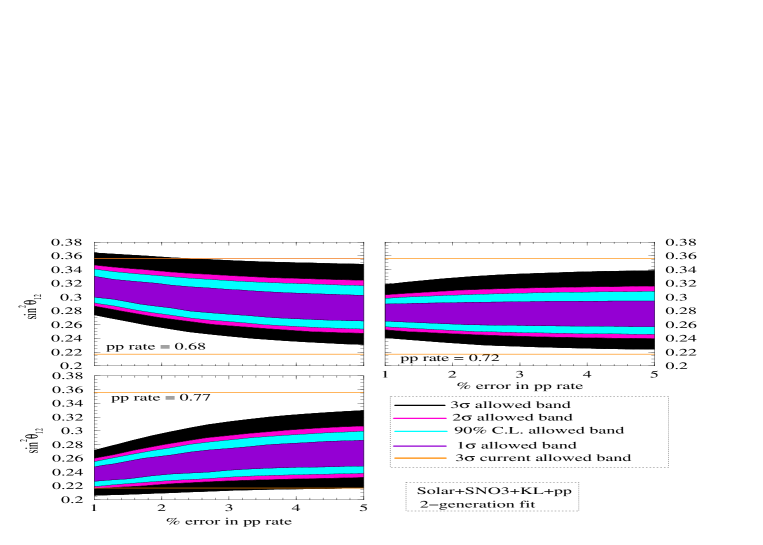
Figure 4: Same as Fig. 3 but including the prospective data (and errors) from the phase-III of SNO experiment.

In Fig. 4 we show the expected range of allowed values of $\sin^{2}\theta_{12}$ as a function of the error in the measured $pp$ rate, after the potential results and projected errors from phase-III of the SNO experiment (SNO3) are included in the global analysis. If the measured mean $pp$ rate is 0.68 (0.77), the maximal (minimal) allowed value of $\sin^{2}\theta_{12}$ slightly increases (decreases) and the minimal (maximal) value increases (decreases) significantly. The total uncertainty in $\sin^{2}\theta_{12}$ is independent of the central value of the $pp$ rate, in agreement, with what we have found earlier. For $R_{pp}=0.72$, the $3\sigma$ spread in $\sin^{2}\theta_{12}$ is $\approx$ 21%, 18%, 18%, 14% for a 4%, 3%, 2% and 1% experimental error in $R_{pp}$, respectively.

It follows from our analysis that the data from the $pp$ experiment can allow to reduce the expected uncertainty of 21% in the determination of $\sin^{2}\theta_{12}$ after the prospective phase-III SNO results are included in the analysis only if the error in the measured $pp$ rate does not exceed $\sim$ 4%. However, even with $\Delta R_{pp}=1\%$, the 3$\sigma$ spread in the value of $\sin^{2}\theta_{12}$ would not be smaller than $\sim$14%.

Table 2 summarises the results on the allowed ranges and spread of $\sin^{2}\theta_{12}$, obtained in a two-neutrino oscillation analysis including SNO-III projected errors. As expected, the spread in $\sin^{2}\theta_{12}$ reduces with inclusion of the phase-III SNO data in the analysis. Note that the ranges given in Table 2 are with the present KamLAND 766.3 Ty spectrum data. If we use future higher statistics data from KamLAND , the allowed spread in $\sin^{2}\theta_{12}$ may reduce somewhat.

		solar+reactor +pp		solar(+SNO3)+reactor+pp
pp rate	% error	3$\sigma$ range	spread	3$\sigma$ range	spread
0.68	1	0.28 - 0.38	15.2%	0.27 - 0.36	14.3%
	2	0.26 - 0.37	17.5%	0.26 - 0.36	16.1%
	3	0.24 -0.37	21.3%	0.24 - 0.35	18.6%
	4	0.24 - 0.37	21.3%	0.23 - 0.35	20.7%
0.72	1	0.24 - 0.32	14.3%	0.24 - 0.32	14.3%
	2	0.23 - 0.33	17.9%	0.23 - 0.32	16.4%
	3	0.23 - 0.34	19.3%	0.23 - 0.33	17.9%
	4	0.22 - 0.35	22.8%	0.22 - 0.34	21.4%
0.77	1	0.20 - 0.27	14.9%	0.20 - 0.27	14.9%
	2	0.21 - 0.30	17.6%	0.21 - 0.29	16.0%
	3	0.21 - 0.32	20.8%	0.21 - 0.31	19.2%
	4	0.21 - 0.33	22.2%	0.21 - 0.32	20.8%

Table 2: The 3$\sigma$ allowed ranges and % spread of $\sin^{2}\theta_{12}$ obtained in a two-neutrino oscillation analysis of the solar neutrino data, including the simulated data on the $pp$ neutrino flux, and the KamLAND 766.3 Ty spectrum data.

3.2 The Impact of Non-Zero $\theta_{13}$

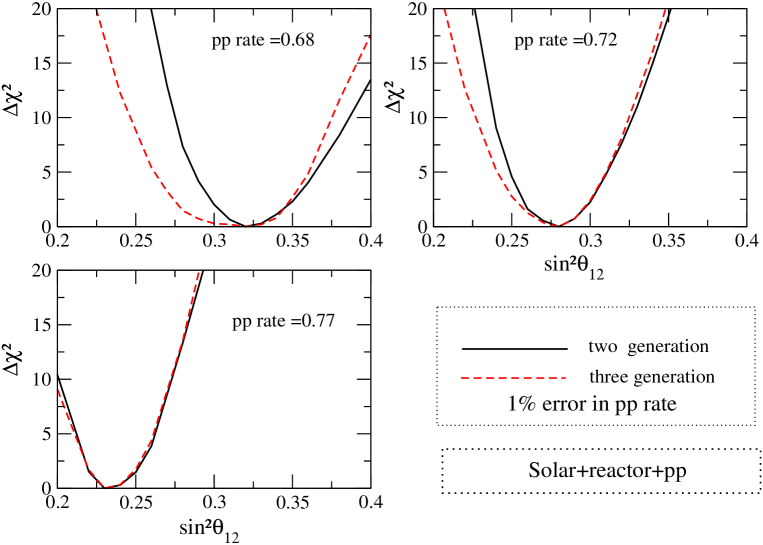
Figure 5: Comparison of $\Delta\chi^{2}$ vs. $\sin^{2}\theta_{12}$ obtained from a two generation analysis (solid black line) and three generation analysis (dashed red line) analyses of the world neutrino data including the $pp$ rate. The three panels show the results for the three illustrative values of the $pp$ rate. We present the results for 1% error in the $pp$ rate. For the three-neutrino oscillation analysis $\sin^{2}\theta_{13}$ is allowed to vary freely.

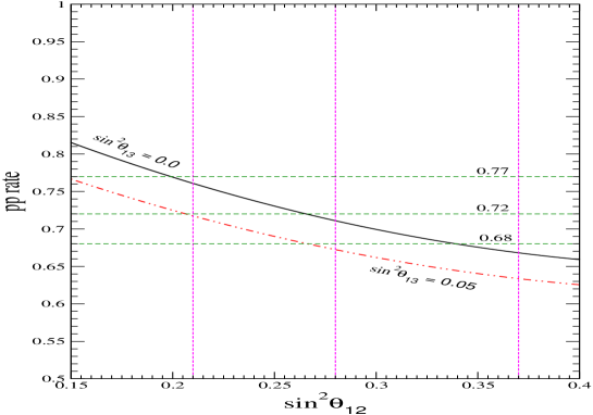
Figure 6: The $pp$ rate as a function of $\sin^{2}\theta_{12}$. The black solid line is the $pp$ rate for $\sin^{2}\theta_{13}=0$ while the red dot-dashed line is $\sin^{2}\theta_{13}=0.05$. We also show our illustrative $pp$ rates of 0.68, 0.72 and 0.77 on the plot.

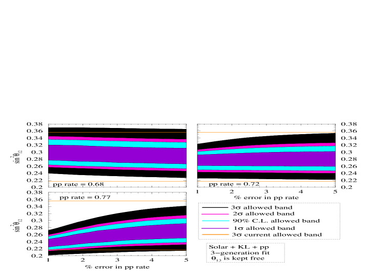
Figure 7: Same as Figure 3 but for a three generation analysis including all neutrino data and keeping $\sin^{2}\theta_{13}$ free. We also show the 3$\sigma$ allowed band of $\sin^{2}\theta_{12}$ from the current data.

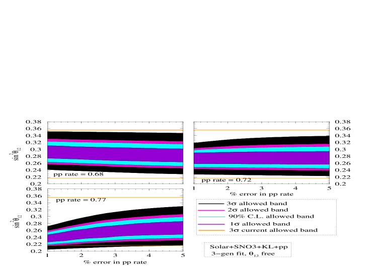
Figure 8: Same as Figure 7 but with the projected error from the third phase of the SNO experiment included. We show the 3$\sigma$ allowed band from current data.

The solar and atmospheric neutrino, K2K and KamLAND data suggest the existence of 3-neutrino mixing and oscillations (see, e.g., [33]). Actually, all existing neutrino oscillation data, except the data of LSND experiment [34], can be described assuming 3-neutrino mixing. This warrants a 3-neutrino oscillation analysis of the potential sensitivity of a LowNu $pp$ neutrino experiment to $\sin^{2}\theta_{12}$.

The 3-neutrino oscillations of interest are characterized by the neutrino mass-squared differences which drive the solar and atmospheric neutrino oscillations, $\Delta m^{2}_{21}=\Delta m^{2}_{\odot}>0$ and $\Delta m^{2}_{31}=\Delta m^{2}_{atm}$ respectively, and by the 3 mixing angles in the Pontecorvo-Maki-Nakagawa-Sakata (PMNS) neutrino mixing matrix, $\theta_{12}$, $\theta_{23}$ and $\theta_{13}$. In the standard parametrization of the PMNS matrix (see, e.g., [33]), the angles $\theta_{12}$ and $\theta_{23}$ coincide with the angles which control the oscillations of solar and atmospheric neutrinos, while $\theta_{13}$ is the angle limited by the data from the CHOOZ and Palo Verde experiments [36]. The precise limit on $\theta_{13}$ depends strongly on $\Delta m^{2}_{atm}$ (see e.g. [37]) The existing atmospheric and reactor neutrino data imply [12, 13]

$$\sin^{2}\theta_{13}<0.05,~{}~{}~{}~{}~{}99.73\%~{}{\rm C.L.}$$ (12)

The aim of the analysis which follows is to quantify the uncertainty which the absence of precise knowledge of the value of the CHOOZ angle $\theta_{13}$ introduces in the precision of $\sin^{2}\theta_{12}$ determination.

The analyses of the latest SK atmospheric neutrino and of the global solar neutrino data show also that [6, 12, 13] $|\Delta m^{2}_{31}|=|\Delta m^{2}_{{\rm atm}}|\sim 2.1\times 10^{-3}~{}{\rm eV^{2}}$ and $\Delta m^{2}_{21}=\Delta m^{2}_{\odot}\sim 8\times 10^{-5}~{}{\rm eV^{2}}$. Thus, we have $\Delta m^{2}_{21}<<|\Delta m^{2}_{31}|$. Under this condition the probabilities of survival of the solar $\nu_{e}$ and of the reactor $\bar{\nu}_{e}$, relevant for the 3-neutrino oscillation interpretation of the solar neutrino and KamLAND data, have the form:

$$P_{ee}^{3\nu}\cong\cos^{4}\theta_{13}P_{ee}^{2\nu}+\sin^{4}\theta_{13}$$ (13)

where $P_{ee}^{2\nu}$ is the corresponding probability of survival of $\nu_{e}$ or $\bar{\nu}_{e}$ in the case of 2-neutrino mixing (see, e.g., [38]). For the reactor $\bar{\nu}_{e}$ detected at KamLAND , $P_{ee}^{2\nu}$ is given by eq. (4). For solar neutrinos, $P_{ee}^{2\nu}\equiv P_{ee\odot}^{2\nu}$ is the $\nu_{e}$ survival probability in the case of 2-neutrino oscillation [39, 31] in which the solar electron number density $N_{e}$ is replaced by $N_{e}\cos^{2}\theta_{13}$. From eqs. (2), (5), (12) and (13) we get:

$$P^{3\nu}_{ee}({\mbox{${}^{8}{B}~{}$}}) \cong \cos^{4}\theta_{13}\sin^{2}\mbox{$\theta_{12}$~{}},$$ (14)

$$P^{3\nu}_{ee}({pp}) \cong \cos^{4}\theta_{13}(1-\frac{1}{2}\sin^{2}2\theta_{12}).$$ (15)

Note that for a given value of $P^{3\nu}_{ee}({pp})$, a non-zero value of $\theta_{13}$ decreases the measured value of $\theta_{12}$, for the low energy $pp$ flux. On the other hand, for a given value of $P^{3\nu}_{ee}({\mbox{${}^{8}{B}~{}$}})$, a non-zero $\theta_{13}$ increases the measured value of $\theta_{12}$, for the higher energy ${}^{8}{B}~{}$ flux.

For $\Delta m^{2}_{21}<<|\Delta m^{2}_{31}|$, the probability relevant for the interpretation of data from the CHOOZ experiment is given by

$$P_{eeCHOOZ}^{3\nu}\approx 1-\sin^{2}2\theta_{13}\sin^{2}(\Delta m_{31}^{2}L/4E).$$ (16)

Note that the probability $P_{eeCHOOZ}^{3\nu}$ depends on $\Delta m^{2}_{31}$, unlike the probabilities relevant for the interpretation of the solar and KamLAND data. In the analysis which we have performed $|\Delta m^{2}_{31}|$ was allowed to vary freely within the $3\sigma$ allowed range given in [6]  .

In Fig. 5 we show the dependence of $\Delta\chi^{2}$ on $\sin^{2}\theta_{12}$, obtained in a 3-neutrino oscillation analysis of the combined KamLAND, CHOOZ and solar neutrino data, including the simulated data on the $pp$ neutrino flux. The results shown are for the three illustrative central values of $R_{pp}$ considered earlier, and for the case of 1% error in $R_{pp}$. Except for $\sin^{2}\theta_{12}$, all the other parameters, including $\sin^{2}\theta_{13}$, were allowed to vary freely in the analysis. For comparison, results for $\sin^{2}\theta_{13}=0$ are shown in the same figure.

We find that

• For a relatively low value of the measured $pp$ rate, $R_{pp}=0.68$, a non-zero $\sin^{2}\theta_{13}$ leads to smaller minimal and maximal allowed values of $\sin^{2}\theta_{12}$.

• For $R_{pp}=0.72$, the minimal allowed value of $\sin^{2}\theta_{12}$ diminishes, while the maximal allowed value remains unaffected.

• If $R_{pp}=0.77$, both values are practically unaffected.

To help explain these features, we plot in Fig. 6 the $pp$ rate (cf. Eqs. (6) and (15)) as a function of $\sin^{2}\theta_{12}$ for $\sin^{2}\theta_{13}=0$ and $\sin^{2}\theta_{13}=0.05$. The three horizontal lines in the figure correspond to the three central values of $R_{pp}$ considered in our analysis. We see from the figure that,

1. For a given value of $\sin^{2}\theta_{12}$, a non-zero $\sin^{2}\theta_{13}$ always reduces the predicted $pp$ rate,

2. For a given measured $pp$ rate, a non-zero $\sin^{2}\theta_{13}$ would reduce the measured value of $\sin^{2}\theta_{12}$,

3. For a given measured $pp$ rate there is always a limiting value of $\sin^{2}\theta_{12}$, such that for $\sin^{2}\theta_{12}$ exceeding this value a non-zero $\sin^{2}\theta_{13}$ does not affect the allowed values of $\sin^{2}\theta_{12}$.

Points (1) and (2) imply, in particular, that if for a given value of $\sin^{2}\theta_{12}$ the $pp$ rate predicted assuming 2-neutrino oscillations is larger than the measured $pp$ rate, a non-zero $\theta_{13}$ can improve the quality of the fit. Thus, values of $\sin^{2}\theta_{12}$ smaller than the minimal allowed one determined in a 2-neutrino oscillation analysis, could become allowed in the case of 3-neutrino oscillations due to non-zero $\sin^{2}\theta_{13}$. As a consequence of point 3 we can conclude that if for a particular value of $\sin^{2}\theta_{12}$, the $pp$ rate predicted in the case of 2-neutrino oscillations is larger than the measured $pp$ rate, a $\sin^{2}\theta_{13}$ which differs from 0 substantially and further lowers the $pp$ rate, would not be favored by the data. We use these features to explain Fig. 5. However it is to be borne in mind that Fig. 6 contains only the pp rates while in Figure 5 we show the results from a combined analysis of global solar and KamLAND data.

• We see from Fig. 6 that the $pp$ rate, predicted in the case of 2-neutrino oscillations, exceeds 0.72 for $\sin^{2}\theta_{12}\ \raisebox{-1.72218pt}{\hbox to0.0pt{$\sim$\hss}}\raisebox{1.72218pt}{$<$}\ 0.27$. Therefore in this case a non-zero $\sin^{2}\theta_{13}$ improves the quality of the fit for all values of $\sin^{2}\theta_{12}\ \raisebox{-1.72218pt}{\hbox to0.0pt{$\sim$\hss}}\raisebox{1.72218pt}{$<$}\ 0.27$. Thus, relatively small values of $\sin^{2}\theta_{12}$ which are disfavored by the 2-neutrino oscillation analysis, could become allowed if $\sin^{2}\theta_{13}\neq 0$. This would lead to a smaller minimal allowed value of $\sin^{2}\theta_{12}$. For $\sin^{2}\theta_{12}>0.27$, the predicted 2-neutrino oscillation rate is already lower than 0.72, and therefore a non-zero $\theta_{13}$ would not change the maximal allowed value of $\sin^{2}\theta_{12}$.

• The predicted $R_{pp}$ for 2-neutrino oscillations can be greater than $R_{pp}=0.77$ only for relatively small values of $\sin^{2}\theta_{12}$, which are strongly disfavored (if not ruled out) by the current data. Consequently, a non-zero $\sin^{2}\theta_{13}$ is not expected to make any impact on the $\sin^{2}\theta_{12}$ determination if the measured $R_{pp}=0.77$.

• In the case of a measured $R_{pp}=0.68$, the predicted 2-neutrino oscillation $pp$ rate is larger than 0.68 for $\sin^{2}\theta_{12}\ \raisebox{-1.72218pt}{\hbox to0.0pt{$\sim$\hss}}\raisebox{1.72218pt}{$<$}\ 0.34$ and a non-zero value of $\sin^{2}\theta_{13}$ can improve the quality of the fit for a large range of values of $\sin^{2}\theta_{12}$. This explains why the minimal allowed value of $\sin^{2}\theta_{12}$ diminishes considerably for $\sin^{2}\theta_{13}\neq 0$ in Fig. 5. The maximal allowed value of $\sin^{2}\theta_{12}$ is also seen to reduce. The reason for this can be understood if one notes that the values of $\sin^{2}\theta_{12}$ favoured by the $pp$ experiment, for $\sin^{2}\theta_{13}=0$, would correspond to a relatively higher value of $R_{CC}/R_{NC}$ compared to that measured at SNO. If $\theta_{13}$ is non-zero, then the same $R_{pp}$ could be produced at a lower value of $\theta_{12}$. Since the predicted $R_{CC}/R_{NC}$ in SNO is given by Eq. (14), this lower $\sin^{2}\theta_{12}$ coupled with non-zero $\theta_{13}$ would help reduce the ${}^{8}B$ probability and the $pp$ “data” could be “reconciled” with the SNO CC/NC data. Therefore for $R_{pp}=0.68$, the best-fit from a three generation analysis comes at a non-zero value of $\sin^{2}\theta_{13}$ and a lower value of $\sin^{2}\theta_{12}$. Note that the value of the global $\chi^{2}_{min}$ for the three generation case ($\theta_{13}\neq 0$) is lower than the two-generation case ($\theta_{13}=0$). However as noted before, since the predicted $R_{pp}$ is already lower than 0.68 for $\sin^{2}\theta_{12}\ \raisebox{-1.72218pt}{\hbox to0.0pt{$\sim$\hss}}\raisebox{1.72218pt}{$>$}\ 0.34$, the $pp$ experiment would force $\theta_{13}=0$ for these high values of $\sin^{2}\theta_{12}$. Thus above $\sin^{2}\theta_{12}\ \raisebox{-1.72218pt}{\hbox to0.0pt{$\sim$\hss}}\raisebox{1.72218pt}{$>$}\ 0.34$ the $\chi^{2}$ remains the same irrespective of whether $\theta_{13}$ was kept free (three-generation) or fixed at zero (two-generation). However, since the global $\chi^{2}_{min}$ was lower for the three-generation fit, the very high values of $\sin^{2}\theta_{12}$, which were allowed in the two-generation analysis get disfavored by the three-generation fit.

In Fig. 7 we depict the $\sin^{2}\theta_{12}$ sensitivity of the world neutrino oscillation data, including the sample data on the $pp$ rate, as a function of % error in the measured $pp$ rate in the case when $\theta_{13}$ is kept free. In Table 3 we give the corresponding 3$\sigma$ ranges of allowed values and spread of $\sin^{2}\theta_{12}$ (columns 3 and 4). A comparison of this figure with Fig. 3 and the Table 3 with Table 2 demonstrates clearly all the specific features associated with the three values of the $pp$ rate discussed above:
For $R_{pp}=0.77$, $\theta_{13}\neq 0$ hardly makes any difference.
For $R_{pp}=0.72$, the minimal allowed value of $\sin^{2}\theta_{12}$ diminishes as a consequence of $\theta_{13}\neq 0$, while the maximal allowed value is unaltered.
For $R_{pp}=0.68$, the inclusion of $\theta_{13}\neq 0$ in the analysis leads to a reduction of both the minimal and maximal allowed values of $\sin^{2}\theta_{12}$.
For $R_{pp}=0.72$ and 0.68 cases we also note that the minimal value of $\sin^{2}\theta_{12}$ increases as the error in $R_{pp}$ increases and the SNO data begins to have a greater influence on the fit.” Thus, the effect of the uncertainty due to $\sin^{2}\theta_{13}$ on the precision of $\sin^{2}\theta_{12}$ measurement decreases as the error in the $pp$ rate increases.

Figure 8 shows the corresponding sensitivity plot of $\sin^{2}\theta_{12}$ from a 3-neutrino oscillation analysis of the global neutrino oscillation data including both the (hypothetical) $pp$ rate data and the prospective data (and errors) from phase-III of the SNO experiment. The corresponding allowed ranges and spread of $\sin^{2}\theta_{12}$ is given in columns 5 and 6 of Table 3.

From the expression of the 3-neutrino oscillation probability, eq. (13), we see that the factor $\cos^{4}\theta_{13}$ acts like a “normalization constant”. Since the current $3\sigma$ limit on this parameter is $\sin^{2}\theta_{13}<0.05$, one would get a $\sim 10\%$ uncertainty in $P_{ee}^{3\nu}$ and would expect similar uncertainty to appear in the value of $\sin^{2}\theta_{12}$ determined using the $pp$ rate. The actual increase in the $\sin^{2}\theta_{12}$ uncertainty due to $\sin^{2}\theta_{13}$ is smaller than $\sim 10\%$, typically being $\sim 3\%$ for the plausible values of the $pp$ rate ($R_{pp}=0.72$) we have considered. Even for the limiting case of $R_{pp}=0.68$, the maximal increase is by $\sim 6\%$

The main reason for this is that when we include both ”low” and ”high” energy experiments in the global analysis there are two conflicting trends. While a non-zero value of $\sin^{2}\theta_{13}$ would have a tendency to lower the value of $\sin^{2}\theta_{12}$ determined from a 2-neutrino oscillation analysis of the data from the $pp$ experiment, but it would also have a tendency to increase the value of $\sin^{2}\theta_{12}$ determined from the data of SNO and SK (i.e., ${}^{8}{B}~{}$neutrino) experiments. At the lower bound, in general, $pp$ tries to shift the fit to non-zero $\sin^{2}\theta_{13}$ and hence lower values of $\sin^{2}\theta_{12}$ but the global data including SNO prevents that. On the other hand, at the upper bound, in general, SNO can push the fit to $\sin^{2}\theta_{13}\neq 0$ and higher $\sin^{2}\theta_{12}$ but $pp$ prefers to keep it at $\sin^{2}\theta_{13}=0.0$ which corresponds to a lower maximal allowed value of $\sin^{2}\theta_{12}$.

The uncertainty in the value of $\sin^{2}\theta_{13}$ leads to an error in $\sin^{2}\theta_{12}$ at the few percent level only when $\sin^{2}\theta_{12}$ is determined using data on the $pp$ rate together with the global solar and reactor neutrino data. Nevertheless, the spread in the value of $\sin^{2}\theta_{12}$ remains well above 12.5% and typically exceeds 16% at $3\sigma$. As we will show in the next section, $\sin^{2}\theta_{12}$ could be measured with a considerably higher precision in a reactor neutrino experiment with a baseline tuned to SPMIN.

		solar+reactor +pp		solar(SNO3)+reactor+pp
pp rate	% error	3$\sigma$ range	spread	3$\sigma$ range	spread
0.68	1	0.24 - 0.37	21.3%	0.24 - 0.35	18.6%
	2	0.23 - 0.37	23.3%	0.24 - 0.35	18.6%
	3	0.23 -0.37	23.3%	0.23 - 0.35	20.7%
	4	0.23 - 0.37	23.3%	0.23 - 0.35	20.7%
0.72	1	0.225 - 0.32	17.4%	0.23 - 0.32	16.4%
	2	0.22 - 0.34	21.4%	0.23 - 0.33	17.9%
	3	0.22 - 0.34	21.4%	0.22 - 0.33	20.0%
	4	0.22 - 0.35	22.8%	0.22 - 0.34	21.4%
0.77	1	0.2 - 0.27	14.9%	0.20 - 0.27	14.9%
	2	0.21 - 0.30	17.6%	0.21 - 0.29	16.0%
	3	0.21 - 0.32	20.8%	0.21 - 0.31	19.2%
	4	0.21 - 0.33	22.2%	0.21 - 0.32	20.8%

Table 3: The 3$\sigma$ allowed ranges and % spread of $\sin^{2}\theta_{12}$, obtained from a 3-neutrino oscillation analysis of the global solar and reactor neutrino data, including the hypothetical data on the $pp$ rate.

4 Measuring $\theta_{12}$ in a Reactor Experiment at SPMIN

In this section we investigate the possibility of measuring the solar neutrino mixing parameter $\sin^{2}\theta_{12}$ in a reactor $\bar{\nu}_{e}$ oscillation experiment, in which the baseline is chosen to correspond to a minimum of the $\bar{\nu}_{e}$ survival probability (SPMIN) [16]. We will consider in what follows an experiment similar to KamLAND , but with a baseline tuned to the SPMIN. The condition of SPMIN reads

$${L_{min}\approx 1.24\frac{E/MeV}{\mbox{$\Delta m_{21}^{2}$~{}}/eV^{2}}}~{}m$$ (17)

For the “old” low-LMA best-fit value of $\Delta m^{2}_{21}=7.2\times 10^{-5}$ eV², the baseline which allows the most accurate measurement of $\sin^{2}\theta_{12}$ was found to be 70 km [16]. For these $\Delta m^{2}_{21}$ and baseline the SPMIN appears at the prompt $e^{+}$ energy of $E_{vis}=3.2$ MeV , $E_{vis}\cong E-0.8$ MeV. The latter corresponds to the maximum of the $e^{+}$ (event) spectrum in the absence of oscillations. Obviously, the energy $E_{vis}\sim 3.2$ MeV, is the most relevant for the statistics of the experiment. We will show in this section that for the current global best-fit value of $\Delta m^{2}_{21}=8.3\times 10^{-5}$ eV², $\sin^{2}\theta_{12}$ could be measured with an accuracy of $\sim 2\%~{}(6\%)$ at $1\sigma~{}(3\sigma)$ if the baseline chosen is $L\sim 60$ km. For $\Delta m^{2}_{21}=8.3\times 10^{-5}$ eV² and $L\sim 60$ km, the SPMIN appears at $E_{vis}=3.2$ MeV in the $e^{+}$ spectrum. We extend our earlier work [16, 41, 18] by investigating in detail the dependence of the precision of $\sin^{2}\theta_{12}$ measurement on the true value of $\Delta m^{2}_{21}$, the baseline, the statistics and on the systematic error of the experiment. We obtain results assuming 2-neutrino oscillations and compare them with the results of a 3-neutrino oscillation analysis. In the latter $\sin^{2}\theta_{13}$ is allowed to vary freely within its currently allowed range. We discuss also the relevance of the geo-neutrino flux for the precision of $\sin^{2}\theta_{12}$ measurement.

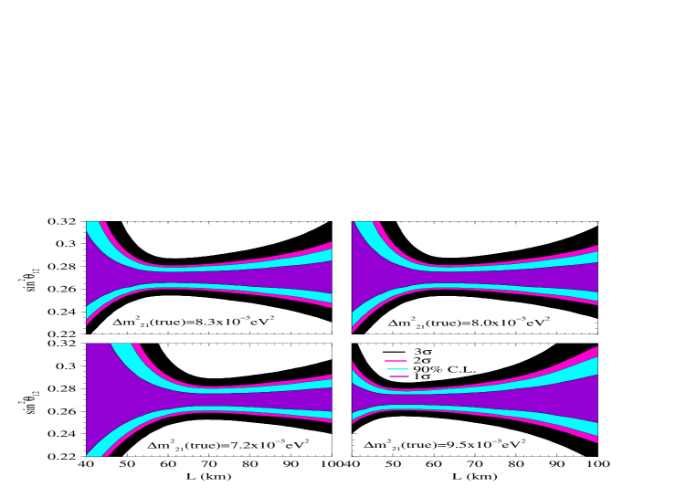
Figure 9: Sensitivity plots showing the $1\sigma$, $1.64\sigma$, $2\sigma$, and $3\sigma$ range of allowed values for $\sin^{2}\theta_{12}$ as a function of the baseline $L$. The 4 panels are for 4 different true value of $\Delta m^{2}_{21}$. The true value of $\sin^{2}\theta_{12}$ is assumed to be 0.27 in all the cases. The $\Delta m^{2}_{21}$ is allowed to vary freely in the fit.

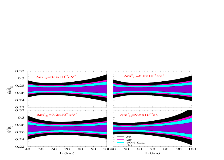
Figure 10: The same as in Fig. 9, but for fixed $\Delta m^{2}_{21}$ having an assumed true value indicated in each of the panels of the figure.

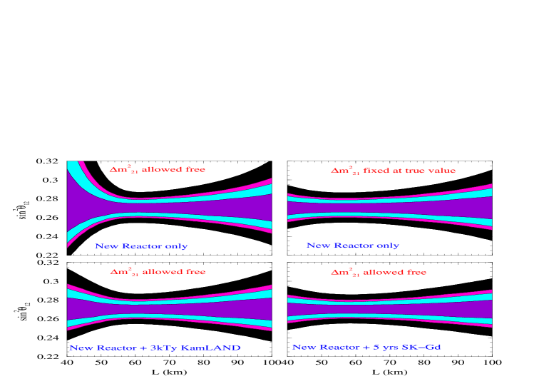
Figure 11: Sensitivity plots showing the $1\sigma$, $1.64\sigma$, $2\sigma$, and $3\sigma$ range of allowed values for $\sin^{2}\theta_{12}$ as a function of the baseline $L$. The true values of $\Delta m^{2}_{21}(true)=8.3\times 10^{-5}$ eV² and of $\sin^{2}\theta_{12}(true)=0.27$ for all panels. The upper left hand (right hand) panel is obtained allowing $\Delta m^{2}_{21}$ to vary freely (for fixed $\Delta m^{2}_{21}(true)=8.3\times 10^{-5}$ eV²). The results shown in the lower left hand (lower right hand) panel are from combined analysis of 3 kTy data from KamLAND (5 year data from the suggested SK-Gd experiment) and 73 GWkTy data from a SPMIN reactor experiment.

4.1 Sensitivity to $\sin^{2}\theta_{12}$ and the Baseline of the Experiment

In Fig. 9 we show the sensitivity to $\sin^{2}\theta_{12}$, expected in a reactor experiment, as a function of the baseline $L$. We assume a total systematic uncertainty of 2% and consider statistics of 73 GWkTy (given as a product of reactor power in GW and the exposure of the detector in kTy). The detector material composition is assumed to be the same as that of KamLAND and so the detector considered has the same number of target protons per kton as KamLAND. The total reactor power, the detector size and the exposure time are kept the same for all baselines. Thus, for longer baseline the number of events would decrease as $\sim L^{-2}$. We assume that the true value of $\sin^{2}\theta_{12}=0.27$ and simulate the prospective observed positron spectrum in the detector for four different assumed true values of $\Delta m^{2}_{21}$. This figure is obtained for $\sin^{2}\theta_{13}=0$.

We define a $\chi^{2}$ function given by

$$\chi^{2}=\sum_{i,j}(N_{i}^{data}-N_{i}^{theory})(\sigma_{ij}^{2})^{-1}(N_{j}^{data}-N_{j}^{theory})~{},$$ (18)

where $N_{i}^{\alpha}$ $(\alpha=data,theory)$ is the number of events in the $i^{\rm th}$ bin, $\sigma_{ij}^{2}$ is the covariant error matrix containing the statistical and systematic errors and the sum is over all bins. We use this $\chi^{2}$ to fit the simulated spectrum data and get the “measured” value of $\sin^{2}\theta_{12}$, keeping $\Delta m^{2}_{21}$ free. We simulate the spectrum at each baseline and plot the range of values of $\sin^{2}\theta_{12}$ allowed by the simulated data as a function of the baseline. The baseline at which the band of allowed values of $\sin^{2}\theta_{12}$ is most narrow is the “ideal” baseline for the SPMIN reactor experiment. The figure confirms that this “ideal” baseline depends critically on the true value of $\Delta m^{2}_{21}$ (cf. eq. (17)). The optimal baseline for the true value of $\Delta m^{2}_{21}=8.3~{}(8.0)\times 10^{-5}$ eV² is seen from Fig. 9 to be $60~{}(63)$ km, while for the “old” low-LMA best-fit value of $\Delta m^{2}_{21}=7.2\times 10^{-5}$ eV² the best baseline would be 70 km. At the optimal baseline the SPMIN reactor experiment can achieve an unprecedented accuracy of $\sim 2\%~{}(6\%)$ at $1\sigma~{}(3\sigma)$ in the measurement of $\sin^{2}\theta_{12}$.

Figure 9 suggests that the optimal baseline for a given true value of $\Delta m^{2}_{21}$ is very finely tuned. For instance, if for $\Delta m^{2}_{21}(true)=8.3\times 10^{-5}$ eV² we change the baseline from $L=60$ to $L=50$ km, the sensitivity in $\sin^{2}\theta_{12}$ decreases from $\sim 2\%~{}(6\%)$ to $\sim 3\%~{}(11\%)$ at $1\sigma~{}(3\sigma)$. However, note that Fig. 9 was obtained by allowing $\Delta m^{2}_{21}$ to vary freely. This is equivalent to assuming that both $\sin^{2}\theta_{12}$ and $\Delta m^{2}_{21}$ are determined in the reactor SPMIN experiment. For some baselines, especially at smaller $L$, the oscillation induced spectral distortion is not large enough to measure $\Delta m^{2}_{21}$ sufficiently accurately, while for the longer baselines the statistics is lower. These factors lead to a certain uncertainty in the determination of $\Delta m^{2}_{21}$ with the experimental set-up under discussion. The uncertainty in the $\Delta m^{2}_{21}$ determination translates into additional uncertainty in the measured $\sin^{2}\theta_{12}$. If $\Delta m^{2}_{21}$ could be measured with a sufficiently high precision in an independent experiment, the uncertainty in $\sin^{2}\theta_{12}$ due to $\Delta m^{2}_{21}$ would be reduced.

Figure 10 represents a sensitivity plot similar to that shown in Fig. 9, but obtained for $\Delta m^{2}_{21}$ fixed at its assumed true value (indicated on each of the panels). As Fig. 10 shows, for fixed $\Delta m^{2}_{21}$ assumed to have been determined with a sufficiently high precision in an independent experiment, the choice of the baseline for setting up the SPMIN experiment becomes broader. It follows from Fig. 10 that for $\Delta m^{2}_{21}(true)=8.3\times 10^{-5}$ eV², for instance, the change of the baseline from $L=60$ to $L=70$ km, leads to a minor increase of the uncertainty in the value of $\sin^{2}\theta_{12}$ from $6.1\%$ to $6.3\%$ at $3\sigma$.

It is actually quite possible that $\Delta m^{2}_{21}$ will be measured with a rather high accuracy in the future. The KamLAND experiment could determine $\Delta m^{2}_{21}$ with an error of about 7% (at 3$\sigma$) using data of 3 kTy [28, 16, 12]. The suggested SK-Gd experiment [42] has the potential of measuring the value of $\Delta m^{2}_{21}$ with an error of $\sim 2-3$% (at 3$\sigma$) [18]. In Fig. 11 we show the sensitivity to $\sin^{2}\theta_{12}$ expected if we combine the SPMIN reactor data with 3 kTy prospective data from KamLAND (lower left panel) and simulated 5 year data from the suggested SK-Gd experiment (lower right panel). The upper panels were obtained using data from the SPMIN reactor experiment alone. For all the panels we have assumed $\Delta m^{2}_{21}(true)=8.3\times 10^{-5}$ eV². In the upper left panel we allow $\Delta m^{2}_{21}$ to vary freely, while in the upper right panel $\Delta m^{2}_{21}$ is fixed at the assumed true value. We note that if the SPMIN reactor data is combined with 5 year data from the SK-Gd experiment, the choice of optimal baseline is much wider since $\Delta m^{2}_{21}$ would be determined with a relatively high precision by the SK-Gd experiment. With the addition of the SK-Gd results to the total data set, the spread in $\sin^{2}\theta_{12}$ is $\sim 5.7\%$ at $3\sigma$. The combined SPMIN reactor and KamLAND 3 kTy data would yield an uncertainty in the value of $\sin^{2}\theta_{12}$ of $\sim 5.9\%$ at $3\sigma$. Since the analysis of the combined KamLAND (or SK-Gd) and SPMIN reactor data confirms that the effect of $\Delta m^{2}_{21}$ on the $\sin^{2}\theta_{12}$ sensitivity can be negligible, we will take $\Delta m^{2}_{21}$ to be fixed for the remainder of this section.

4.2 Impact of Statistical and Systematic Errors on $\sin^{2}\theta_{12}$ Sensitivity

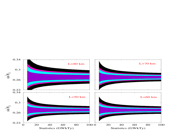
Figure 12: Sensitivity plots showing the $1\sigma$, $1.64\sigma$, $2\sigma$, and $3\sigma$ ranges of allowed values for $\sin^{2}\theta_{12}$ as a function of the statistics in units of GWkTy. All the four panels correspond to a fixed value of $\Delta m^{2}_{21}=8.3\times 10^{-5}$ eV².

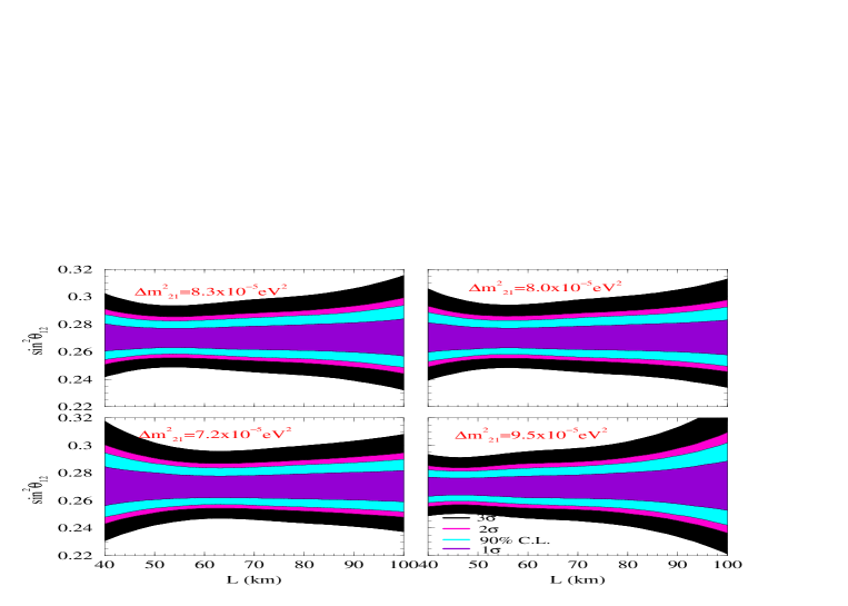
Figure 13: The Same as in Fig. 10 but for a systematic uncertainty of 5%.

One of the important requirements for the type of high precision experiment we are discussing is the accumulation of relatively high statistics in a reasonable period of time. Since the statistics falls as $\sim L^{-2}$ and since rather long baselines are required for a precision measurement of the solar neutrino oscillation parameters, for a given reactor power longer baselines would imply bigger detectors and larger exposure times. Thus, the question about the dependence of the precision of measurement of $\sin^{2}\theta_{12}$ in a reactor SPMIN experiment on the statistics of the experiment naturally arises. In Fig. 12 we show the effect of the statistics on the $\sin^{2}\theta_{12}$ sensitivity in the case of $\Delta m^{2}_{21}(true)=8.3\times 10^{-5}$ eV². The four panels are obtained for four different sample baselines of 50, 60, 70 and 80 km. The range of allowed values of $\sin^{2}\theta_{12}$ is shown as a function of the product of reactor power and the detector mass and exposure time. For $L=60$ km, for instance, the uncertainty in $\sin^{2}\theta_{12}$ diminishes from 3% (10%) to 2% (6%) at $1\sigma(3\sigma)$ as the statistics is increased from 20 GWkTy to 60 GWkTy. Note that the difference in the $\sin^{2}\theta_{12}$ precision for 60 GWkTy and 73 GWkTy (used in Figs. 9 and 10) is marginal, and shows up only in the first place in decimal in the value of the spread.

Another important aspect which determines the potential of the experiment for precision measurement of $\sin^{2}\theta_{12}$ is the systematic uncertainty. Obviously, smaller systematic errors are preferable. All the plots presented so far in this section have been generated with an assumed 2% systematic error. The systematic uncertainty in the KamLAND experiment is about 6.5%. Most of it comes from the uncertainty in the detector fiducial mass and the reactor power. Our choice of 2% for the systematic error is based on the optimistic assumption that the error in the flux normalization could be reduced sufficiently by using the near-far detector set-up. One could envisage the $\theta_{12}$ reactor SPMIN experiment as a second leg of a reactor experiment dedicated to measure $\theta_{13}$ (see, e.g., [43]). The detector for measuring $\theta_{13}$ could then effectively be used as near detector for the long baseline SPMIN experiment for high precision measurement of $\theta_{12}$. It should be added that the errors due to the uncertainties in the threshold energy and $\bar{\nu}_{e}$ spectrum have also to be reduced to achieve the systematic error of 2%. Experimentally this could be a very challenging task.

Since systematic uncertainties may be difficult to reduce in the experiment under discussion, we estimate next how much the precision on $\sin^{2}\theta_{12}$ deteriorates as the systematic error increases. Figure 13 shows the effect of increasing the systematic error from the 2% assumed by us to the rather conservative value of 5%. For $\Delta m^{2}_{21}(true)=8.3\times 10^{-5}$ eV², the spread in $\sin^{2}\theta_{12}$ at $L=60$ km increases from 6.1% to 8.6% at $3\sigma$, as the systematic error is increased from 2% to 5%. We conclude that the effect of systematic uncertainty on the precision of $\sin^{2}\theta_{12}$ measurement is important, but its impact is not dramatic as long as the systematic error does not exceed 5%. Similar conclusion regarding the effect of a 4% systematic error on the accuracy of $\sin^{2}\theta_{12}$ determination in the SADO experiment was reached in [23].

4.3 The Uncertainty Due to $\sin^{2}\theta_{13}$

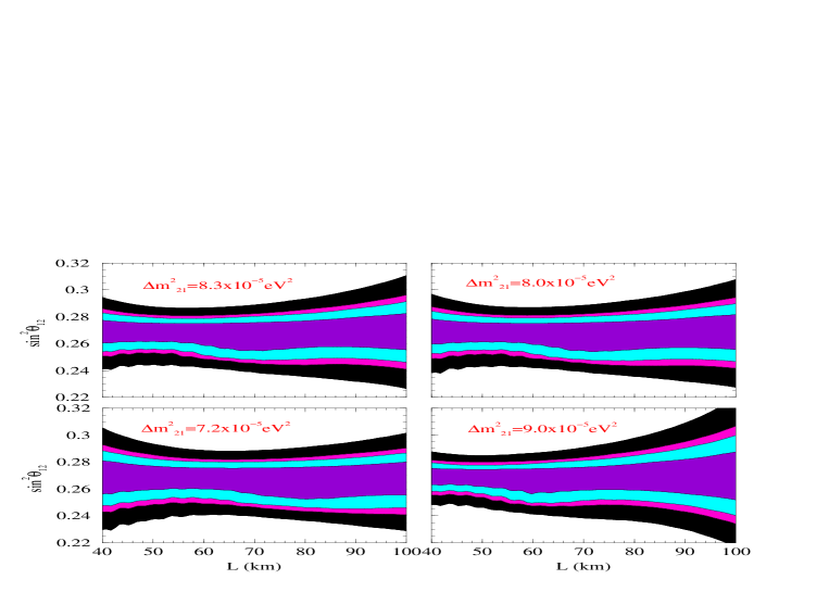
Figure 14: The same as in Fig. 10 but for a 3-neutrino oscillation analysis in which $\sin^{2}\theta_{13}$ is allowed to vary freely within its current $3\sigma$ allowed range.

As we have discussed earlier in connection with the KamLAND experiment, the 3-neutrino oscillation survival probability for the reactor $\bar{\nu}_{e}$ of interest is given by

$$P_{ee}\approx\cos^{4}\theta_{13}\left(1-\sin^{2}2\theta_{12}\sin^{2}\frac{\Delta{m}^{2}_{21}\,L}{4\,E_{\nu}}\right)~{},$$ (19)

where the term $\sim\sin^{4}\theta_{13}$ has been neglected. Therefore the uncertainty in $\sin^{2}\theta_{13}$, eq. (12), brings up to a $\sim 10\%$ uncertainty in the value of the $\bar{\nu}_{e}$ survival probability. Since the factor $\cos^{4}\theta_{13}$ can only reduce the survival probability, it does not affect the upper limit of the allowed range of $\sin^{2}\theta_{12}$. However, it can have an effect on the minimal allowed value of $\sin^{2}\theta_{12}$ reducing it further, and thus can worsen, in principle, the precision of the experiment to $\sin^{2}\theta_{12}$.

The additional error on $\sin^{2}2\theta_{12}$ coming from the uncertainty in $\sin^{2}\theta_{13}$ can be roughly estimated using eq. (19) as [41],

$$\delta(\sin^{2}2\theta_{12})\approx\frac{2\Delta P_{ee}\sin^{2}\theta_{13}}{\sin^{2}\frac{\Delta{m}^{2}_{21}\,L}{4\,E_{\nu}}}+2~{}\frac{(1-\sin^{2}2\theta_{12}~{}\sin^{2}\frac{\Delta{m}^{2}_{21}\,L}{4\,E_{\nu}})~{}\Delta(\sin^{2}\theta_{13})}{\sin^{2}\frac{\Delta{m}^{2}_{21}\,L}{4\,E_{\nu}}}~{},$$ (20)

where $\Delta P_{ee}$ and $\Delta(\sin^{2}\theta_{13})$ are the uncertainties in the determination of the survival probability and $\sin^{2}\theta_{13}$, respectively. In the SPMIN region we are interested in one has $\sin^{2}(\Delta{m}^{2}_{21}L/4E_{\nu})\sim 1$ and therefore

$$\delta(\sin^{2}2\theta_{12})\approx 2\Delta P_{ee}\sin^{2}\theta_{13}+2~{}\cos^{2}2\theta_{12}~{}\Delta(\sin^{2}\theta_{13})~{}.$$ (21)

Thus, for a reactor SPMIN set-up, the first term gives an extra contribution of about $2\Delta P_{ee}\sin^{2}\theta_{13}$ to the allowed range of $\sin^{2}2\theta_{12}$. Even under the most conservative conditions one can expect that $\Delta P_{ee}\ \raisebox{-1.72218pt}{\hbox to0.0pt{$\sim$\hss}}\raisebox{1.72218pt}{$<$}\ 0.1$, so this term could give an additional contribution of $\ \raisebox{-1.72218pt}{\hbox to0.0pt{$\sim$\hss}}\raisebox{1.72218pt}{$<$}\ 0.01$ to the allowed range of $\sin^{2}2\theta_{12}$. The second term is independent of the precision of a given experiment. It depends only on the best-fit value of $\cos^{2}2\theta_{12}$ and on the uncertainty in $\sin^{2}\theta_{13}$. For the current $3\sigma$ upper limit on $\sin^{2}\theta_{13}$ of 0.05 and best-fit value of $\cos^{2}2\theta_{12}=0.19$, the second term would lead to an increase in the uncertainty in $\sin^{2}2\theta_{12}$ by about 0.02 only. The suppression of this term is mainly due to the presence of the $\cos^{2}2\theta_{12}$ factor, which is relatively small for the current best-fit value. Thus, even though the current uncertainty in $\sin^{2}\theta_{13}$ brings a 10% uncertainty in the value of $P_{ee}$, it increases the allowed range of $\sin^{2}2\theta_{12}$ only by a few %, if one uses a reactor experiment with a baseline tuned to the SPMIN for a high precision measurement of $\sin^{2}2\theta_{12}$.

The above conclusions are illustrated in Fig. 14 showing the uncertainty in $\sin^{2}\theta_{12}$ expected in the case when $\theta_{13}$ is allowed to vary freely in its currently allowed range of $\sin^{2}\theta_{13}<0.05$. The figure confirms that the upper bound on $\sin^{2}\theta_{12}$ remains unaffected by the $\sin^{2}\theta_{13}$ uncertainty, while the minimal allowed value diminishes somewhat, increasing the uncertainty in $\sin^{2}\theta_{12}$. However, for the baseline which corresponds to the SPMIN, the sensitivity reduces only by $2-3\%$ in spite of the 10% uncertainty in $\sin^{2}\theta_{13}$. For $\Delta m^{2}_{21}(true)=8.3\times 10^{-5}$ eV², for instance, the uncertainty in $\sin^{2}\theta_{12}$ increases from 6.1% to 8.7% at $3\sigma$.

4.4 On the Impact of Geo-Neutrino Flux

Our Earth is known to be a huge heat reservoir and is estimated to radiate about 40 TW of heat. A large fraction ($\sim 16\%$) of this is believed to be radiogenic in origin, coming from the decay chain of ${}^{238}U$, ${}^{232}Th$ and ${}^{40}K$. The radioactive decays of these isotopes produce antineutrinos in the beta decay processes of their decay chains. These ${\bar{\nu}_{e}}$ coming from inside the Earth are usually called Geo-neutrinos ($\bar{\nu}^{geo}_{e}$) [44]. The maximum energy of the $\bar{\nu}^{geo}_{e}$ produced in the ${}^{40}K$ decay chain is only $E_{\bar{\nu}_{e}}=1.31$ MeV, which is below the detection energy threshold of ${\bar{\nu}_{e}}$ in scintillation detectors of the type of KamLAND we are considering. However, the $\bar{\nu}^{geo}_{e}$ from ${}^{238}U$ and ${}^{232}Th$ have maximum energy of $E_{\bar{\nu}_{e}}=3.26$ MeV and $E_{\bar{\nu}_{e}}=2.25$ MeV, respectively, and can be observed in scintillation detectors.

The flux of $\bar{\nu}^{geo}_{e}$ is unknown. Even the total heat radiated by Earth has a rather large uncertainty: it could be $31-40$ TW. There is no direct measurement of the abundances of the ${}^{238}U$ and ${}^{232}Th$ inside the Earth. One can estimate their abundances using the meteoritic and seismic data. This results in the $\bar{\nu}^{geo}_{e}$ flux being largely model dependent and uncertain. Most models give the bulk ${}^{232}Th$/${}^{238}U$ ratio as ${}^{232}Th$/${}^{238}U\sim 3.8$. Even the value of this ratio could have a realtively large error (e.g., the authors of [45] estimate this error as 14%). The measurement of the $\bar{\nu}^{geo}_{e}$ flux would lead to a better understanding of the interior of the Earth, and is therefore a very important branch of neutrino physics in its own right [46]. As far as the precision measurement of the neutrino oscillation parameters is concerned, the events due to $\bar{\nu}^{geo}_{e}$ can be an important background and can lead to an error in the measured value of $\sin^{2}\theta_{12}$.

Since the $\bar{\nu}^{geo}_{e}$ have a maximum energy of $E_{\bar{\nu}_{e}}=3.26$ MeV which corresponds to a prompt $e^{+}$ energy of only $E_{vis}=2.48$ MeV, one way to avoid the uncertainty due to $\bar{\nu}^{geo}_{e}$ is to implement a prompt energy threshold of 2.6 MeV, as is done by the KamLAND collaboration. In this paper we have followed the KamLAND approach. In this case the observed $e^{+}$ spectrum does not have any “contamination” due to contributions from $\bar{\nu}^{geo}_{e}$. An alternative approach is to use the entire prompt $e^{+}$ energy spectrum in the analysis, taking the $\bar{\nu}^{geo}_{e}$ flux into account. Since the theoretical estimates on the $\bar{\nu}^{geo}_{e}$ flux are presently rather imprecise, one could let the ${}^{238}U$ and ${}^{232}Th$ $\bar{\nu}^{geo}_{e}$ flux normalisation vary as a free parameter. Both approaches have their merits and drawbacks. In the first approach (we use in this paper), while there are no additional uncertainties due to the unknown $\bar{\nu}^{geo}_{e}$ background, one has to contend with the experimental challenge of understanding and reducing the error associated with the prompt $e^{+}$ threshold energy. In the case of KamLAND experiment the uncertainty in the $e^{+}$ threshold energy corresponds to a systematic error $\sim$2.3%. In the second approach there is no prompt $e^{+}$ energy cut, but one has to handle the uncertainty due to the lack of knowledge of $\bar{\nu}^{geo}_{e}$ background. Keeping the ${}^{238}U-$ and ${}^{232}Th-$ $\bar{\nu}^{geo}_{e}$ flux normalisation as free parameter brings in extra error in the measurement on $\sin^{2}\theta_{12}$.

The key feature in the $\theta_{12}$ SPMIN reactor experiment suggested in [16], is the appearance of SPMIN in the observed $e^{+}$ spectrum. If the SPMIN appears at a prompt energy of $E_{vis}>2.6$ MeV, implementing a threshold of $E_{vis}=2.6$ MeV and thus avoiding the $\bar{\nu}^{geo}_{e}$ background might permit to measure $\sin^{2}\theta_{12}$ with the highest precision, achievable in the experiment under discussion. If, on the other hand, SPMIN appears at $E_{vis}<2.6$ MeV, the entire $e^{+}$ energy spectrum would have to be taken into account and in this case the $\bar{\nu}^{geo}_{e}$ background cannot be avoided. For a given value of $\Delta m^{2}_{21}$, the position of the SPMIN in the ${\bar{\nu}_{e}}$ spectrum depends on the baseline of the experiment. For shorter baselines, SPMIN occurs at smaller energies. Therefore the choice of the baseline of the experiment would determine whether one would have to take the $\bar{\nu}^{geo}_{e}$ background into account or not.

The authors of [23] have included the $\bar{\nu}^{geo}_{e}$ background in their analysis of the $\sin^{2}\theta_{12}$ precision expected in the SADO experiment in Japan with a baseline of $L=54$ km. They conclude that for this experimental set-up, the $\bar{\nu}^{geo}_{e}$ background does not have significant impact on the precision of $\sin^{2}\theta_{12}$ measurement. For $L=54$ km, the SPMIN is at $E_{vis}\cong 2.8$ MeV. The uncertainty in the $\bar{\nu}^{geo}_{e}$ flux does not make much impact in this case since $E_{vis}\cong 2.8$ MeV is larger than the background $\bar{\nu}^{geo}_{e}$ energies. For shorter baselines the SPMIN will take place at $E_{vis}<2.6$ MeV and the uncertainty due to the $\bar{\nu}^{geo}_{e}$ flux can affect noticeably the precision of measurement of $\sin^{2}\theta_{12}$.

5 Conclusions

We have investigated the possibilities of high precision measurement of the solar neutrino mixing angle $\theta_{12}$ in solar and reactor neutrino experiments. As a first step, we have analyzed the improvements in the determination of $\sin^{2}\theta_{12}$, which can be achieved with the expected increase of statistics and reduction of systematic errors in the currently operating solar and KamLAND experiments. With the phase-III prospective data from SNO experiment included in the current global solar neutrino and KamLAND data, the uncertainty in the value of $\sin^{2}\theta_{12}$ is expected to diminish from 24% to 21% at 3$\sigma$. If instead of 766.3 Ty, one uses simulated 3 kTy KamLAND data in the same analysis, the 3$\sigma$ error in $\sin^{2}\theta_{12}$ reduces to 18%.

We next considered the potential of a generic LowNu $\nu-e$ elastic scattering experiment, designed to measure the $pp$ solar neutrino flux, for high precision determination of $\sin^{2}\theta_{12}$. We examined the effect of including values of the $pp$ neutrino induced electron scattering rates in the $\chi^{2}$ analysis of the global solar neutrino data. Three representative values of the rates from the currently allowed 3$\sigma$ range were considered: 0.68, 0.72, 0.77. The error in the measured rate was varied from 1% to 5%. By adding the $pp$ flux data in the analysis, the error in $\sin^{2}\theta_{12}$ determination reduces to 14% (19%) at 3$\sigma$ for 1% (3%) uncertainty in the measured $pp$ rate. Performing a similar three-neutrino oscillation analysis we found that, as a consequence of the uncertainty on $\sin^{2}\theta_{13}$, the error on the value of $\sin^{2}\theta_{12}$ increases correspondingly to 17% (21%).

We also studied the possibility of a high precision determination of $\sin^{2}\theta_{12}$ in a reactor experiment with a baseline corresponding to a Survival Probability MINimum (SPMIN). We showed that in a $L\sim 60$ km experiment with statistics of $\sim$60 GWkTy and systematic error of 2%, $\sin^{2}\theta_{12}$ could be measured with an uncertainty of 2% (6%) at 1$\sigma$ (3$\sigma$). The inclusion of the $\sin^{2}\theta_{13}$ uncertainty in the analysis changes this error to 3% (9%). An independent determination of $\Delta m^{2}_{21}$ with sufficiently high accuracy would allow, as we have shown, $\sin^{2}\theta_{12}$ to be measured with the highest precision over a relatively wide range of baselines. We investigated in detail the dependence of the precision on $\sin^{2}\theta_{12}$ which can be achieved in such an experiment on the baseline, statistics and systematic error. More specifically, with the increase of the statistics from 20 GWkTy to 60 GWkTy, the error diminishes from 3% (10%) to 2% (6%) at 1$\sigma$ (3$\sigma$). For statistics of (60 - 70) GWkTy, the increase of the systematic error from 2% to 5% leads to an increase in the uncertainty in $\sin^{2}\theta_{12}$ from 6% to 9% at 3$\sigma$.

We have found that the effect of $\sin^{2}\theta_{13}$ uncertainty on the $\sin^{2}\theta_{12}$ determination in LowNu $pp$ and SPMIN reactor experiments considered is considerably smaller than naively expected.

The results of our analyses for the currently running, the proposed LowNu and future reactor experiments show that the most precise determination of $\sin^{2}\theta_{12}$ can be achieved in a dedicated reactor experiment with a baseline tuned to SPMIN associated with $\Delta m^{2}_{21}\equiv\Delta m^{2}_{\odot}$.

Acknowledgments: We would like to thank Y. Suzuki, A. Suzuki, M. Nakahata, F. Suekane, and C. Peña-Garay for useful discussions. This work was supported by the Italian INFN under the program “Fisica Astroparticellare” (S.C. and S.T.P.).

References

- [1] B. T. Cleveland et al., Astrophys. J. 496, 505 (1998).
- [2] J. N. Abdurashitov et al. [SAGE Collaboration], J. Exp. Theor. Phys. 95, 181 (2002) [Zh. Eksp. Teor. Fiz. 122, 211 (2002)] [arXiv:astro-ph/0204245]. ; W. Hampel et al. [GALLEX Collaboration], Phys. Lett. B 447, 127 (1999); C. Cattadori, Talk at Neutrino 2004, Paris, France, June 14-19, 2004 (http://neutrino2004.in2p3.fr).
- [3] S. Fukuda et al. [Super-Kamiokande Collaboration], Phys. Lett. B 539, 179 (2002).
- [4] Q. R. Ahmad et al. [SNO Collaboration], Phys. Rev. Lett. 89, 011301 (2002). Q. R. Ahmad et al. [SNO Collaboration], Phys. Rev. Lett. 89, 011302 (2002) [arXiv:nucl-ex/0204009].
- [5] S. N. Ahmed et al. [SNO Collaboration], Phys. Rev. Lett. 92, 181301 (2004).
- [6] E. Kearns, talk at Neutrino 2004, Paris, (http://neutrino2004.in2p3.fr).
- [7] K. Eguchi et al., [KamLAND Collaboration], Phys.Rev.Lett.90 (2003) 021802.
- [8] M.H. Ahn et al., Phys.Rev.Lett. 90 (2003) 041801.
- [9] T. Araki et al., [KamLAND Collaboration], hep-ex/0406035.
- [10] T. Nakaya et al., talk given at ’04 International Conference, June 14-19, 2004, Paris, France (http://neutrino2004.in2p3.fr).
- [11] V. Gribov and B. Pontecorvo, Phys. Lett. B28, 493 (1969).
- [12] A. Bandyopadhyay, S. Choubey, S. Goswami, S. T. Petcov and D. P. Roy, hep-ph/0406328.
- [13] M. Maltoni, T. Schwetz, M. A. Tortola and J. W. F. Valle, arXiv:hep-ph/0405172; J. N. Bahcall, M. C. Gonzalez-Garcia and C. Pena-Garay, JHEP 0408, 016 (2004); P. Aliani, V. Antonelli, R. Ferrari, M. Picariello and E. Torrente-Lujan, arXiv:hep-ph/0406182.
- [14] B. Aharmim et al. [SNO Collaboration], arXiv:nucl-ex/0502021.
- [15] A. Bandyopadhyay et al. work in progress.
- [16] A. Bandyopadhyay, S. Choubey and S. Goswami, Phys. Rev. D 67, 113011 (2003).
- [17] A. Bandyopadhyay, S. Choubey, S. Goswami and S. T. Petcov, Phys. Lett. B 581, 62 (2004).
- [18] S. Choubey and S. T. Petcov, Phys. Lett. B 594, 333 (2004).
- [19] R. S. Raghavan, Talk given at the Int. Workshop on Neutrino Oscillations and their Origin (NOON2004), February 11 - 15, 2004, Tokyo, Japan; for further information see the web-site: http://www.phys.vt.edu/ kimballton/ .
- [20] M. Nakahata, Talk given at the Int. Workshop on Neutrino Oscillations and their Origin (NOON2004), February 11 - 15, 2004, Tokyo, Japan.
- [21] Y. Suzuki, Talk given at ’04 International Conference, June 14-19, 2004, Paris, France (http://neutrino2004.in2p3.fr).
- [22] J. N. Bahcall and C. Pena-Garay, JHEP 0311, 004 (2003).
- [23] H. Minakata, H. Nunokawa, W. J. C. Teves and R. Zukanovich Funchal, arXiv:hep-ph/0407326.
- [24] J. N. Bahcall and M. H. Pinsonneault, Phys. Rev. Lett. 92, 121301 (2004).
- [25] A. Bandyopadhyay, S. Choubey, S. Goswami and K. Kar, Phys. Lett. B 519, 83 (2001).
- [26] A. Bandyopadhyay, S. Choubey, S. Goswami and D. P. Roy, Phys. Lett. B 540, 14 (2002). S. Choubey, A. Bandyopadhyay, S. Goswami and D. P. Roy, arXiv:hep-ph/0209222.
- [27] A. Bandyopadhyay, S. Choubey, S. Goswami, S. T. Petcov and D. P. Roy, Phys. Lett. B 583, 134 (2004).
- [28] A. Bandyopadhyay, S. Choubey, R. Gandhi, S. Goswami and D. P. Roy, J. Phys. G 29, 2465 (2003) [arXiv:hep-ph/0211266]. A. Bandyopadhyay, S. Choubey, R. Gandhi, S. Goswami and D. P. Roy, Phys. Lett. B 559, 121 (2003).
- [29] Kevin Graham, talk at NOON 2004, February 11-15, 2004, Tokyo, Japan, http://www-sk.icrr.u-tokyo.ac.jp/noon2004/; H. Robertson for the SNO Collaboration, Talk given at TAUP 2003, Univ. of Washington, Seattle, Washington, September 5 - 9, 2003, http://mocha.phys.washington.edu/taup2003
- [30] M. Maris and S.T. Petcov, Phys. Lett. B 534, 17 (2002).
- [31] S.T. Petcov and J. Rich, Phys. Lett. B 224, 401 (1989).
- [32] G.L. Fogli and E. Lisi, Astropart. Phys. 3, 185 (1995).
- [33] S.T. Petcov, New. J. Phys. 6 (2004) 109 (http://stacks.iop.org/1367-2630/6/109), and Talk given at XXIst International Conference on Neutrino Physics and Astrophysics (Neutrino-2004), June 14-19, 2004, Paris, France (see http://neutrino2004.in2p3.fr).
- [34] C. Athanassopoulos et al., Phys. Rev. Lett. 81 (1998) 1774.
- [35] S. Brice et al., Talk given at ’04 International Conference, June 14-19, 2004, Paris, France (http://neutrino2004.in2p3.fr).
- [36] M. Apollonio et al. [CHOOZ Collaboration], Phys. Lett. B 466, 415 (1999), and periment,” Eur. Phys. J. C 27, 331 (2003); F. Boehm et al., Phys. Rev. D 64, 112001 (2001).
- [37] S. Goswami, Global analysis of neutrino oscillation, talk at XXIst International Conference on Neutrino Physics and Astrophysics (Neutrino-2004), Paris, June 14-19, 2004, see http://neutrino2004.in2p3.fr/ ; S. Goswami, A. Bandyopadhyay, S. Choubey [hep-ph/0409224].
- [38] S.T. Petcov, Phys. Lett. B 214, 259 (1988).
- [39] S.T. Petcov, Phys. Lett. B 200, 373 (1988), and Phys. Lett. B 214, 139 (1988); P.I. Krastev and S.T. Petcov, Phys. Lett. B 207, 64 (1988); E. Lisi et al., Phys. Rev. D 63, 093002 (2000).
- [40] A. Bandyopadhyay, S. Choubey, S. Goswami and K. Kar, Phys. Rev. D 65, 073031 (2002).
- [41] S. Choubey, S. T. Petcov and M. Piai, Phys. Rev. D 68, 113006 (2003).
- [42] J. F. Beacom and M. R. Vagins, arXiv:hep-ph/0309300.
- [43] K. Anderson et al., White Paper Report on Using Nuclear Reactors to Search for , arXiv:hep-ex/0402041.
- [44] G. Eder, Nucl. Phys. 78, 657 (1966).
- [45] G. L. Fogli, E. Lisi, A. Palazzo and A. M. Rotunno, arXiv:hep-ph/0405139.
- [46] G. Fiorentini, M. Lissia, F. Mantovani and R. Vannucci, arXiv:hep-ph/0409152. F. Mantovani, L. Carmignani, G. Fiorentini and M. Lissia, Phys. Rev. D 69, 013001 (2004); G. Fiorentini, T. Lasserre, M. Lissia, B. Ricci and S. Schonert, Phys. Lett. B 558, 15 (2003); H. Nunokawa, W. J. C. Teves and R. Zukanovich Funchal, JHEP 0311, 020 (2003).