Rare top quark and Higgs boson decays in Alternative Left-Right Symmetric Models

Abstract

Top quark and Higgs boson decays induced by flavor-changing neutral currents (FCNC) are very much suppressed in the Standard Model (SM). Their detection in colliders like the Large Hadron Collider (LHC), Next Linear Collider (NLC) or Tevatron would be a signal of new physics. We evaluate the FCNC decays $t\rightarrow H^{0}+c$, $t\rightarrow Z+c$, and $H^{0}\rightarrow t+{\bar{c}}$ in the context of Alternative Left-Right symmetric Models (ALRM) with extra isosinglet heavy fermions; in this case, FCNC decays occurs at tree-level and they are only suppressed by the mixing between ordinary top and charm quarks, which is poorly constraint by current experimental values. This provides the possibility for future colliders, either to detect new physics, or to improve present bounds on the parameters of the model.

I Introduction

Rare top quark decays are interesting because they might be a source of possible new physics effects. Due to its large mass of about $178\,GeV$ Abazov:2004cs , the top quark dominant decay mode is into the channel $t\rightarrow b+W$. In the Standard Model (SM), based on the spontaneously broken local symmetry $SU(3)_{C}\otimes SU(2)_{L}\otimes U(1)_{Y}$, flavor-changing neutral currents (FCNC) are absent at the tree-level due to the Glashow-Iliopoulos-Maiani (GIM) mechanism, and they are extremely small at loop level. However, new FCNC states can appear in top decays if there is physics beyond the Standard Model. Moreover, in some particular models beyond the SM, rare top decays may be significantly enhanced to reach detectable levels Bejar1 .

Rare top decays have been studied in the context of the SM and beyond Jenkins ; Mele ; Diaz:91 . The top quark decays into gauge bosons ($t\rightarrow c+V;\,V\equiv\gamma,\,Z,\,g$) are extremely rare events in the SM; their branching ratios are, according to Ref. Diaz:91 ; Eilam : $5\times 10^{-13}$ for the photon, $10^{-13}$ for the Z-boson and $\sim 4\times 10^{-11}$ for the gluon channel, and even smaller according to other estimates Aguilar . Similarly, the top quark decay into the SM Higgs boson, is a very rare decay, with $BR\,(t\rightarrow c+H)\sim 10^{-14}$ Mele ; EilamE . However, by considering physics beyond the SM, for example, the Minimal Supersymmetric Standard Model (MSSM) or the two-Higgs-doublet model (2HDM) or extra quark singlets, new possibilities open up Bejar1 ; Jenkins ; Mele ; Han ; Eilam ; Aguilar ; EilamE ; Herrero ; Aguilar-Saavedra:2002kr , enhancing this branching ratios to the order of $\sim 10^{-6}$ for the $t\to c+Z$ Aguilar channel and $\sim 10^{-4}$ for the $t\to c+H$ Herrero case. The rare top decay $t\rightarrow q+W+Z$ has also been considered as a future test of new physics Diaz .

On the other hand, the FCNC decays of the Higgs boson can be important in various scenarios, including the MSSM Hou . The FCNC Higgs decay into a top quark within a general 2HDM has been studied in Ref. Bejar2 . Because the FCNC Higgs decays in the SM are very suppressed, any experimental signature of Higgs FCNC type could be evidence of physics beyond the SM.

In the future CERN Large Hadron Collider (LHC), about $10^{7}$ top quark pairs will be produced per year Beneke . An eventual signal of FCNC in the top quark decay will have to be ascribed to new physics. Furthermore, since the Higgs boson could also be produced at significant rates in future colliders, it is also important to search for all the relevant FCNC Higgs decays.

On the other hand, while the electroweak SM has been successful in the description of low-energy phenomena, it leaves many questions unanswered. One of them has to do with the understanding of the origin of parity violation in low-energy weak interaction processes. Within the framework of left-right symmetric models, based on the gauge group $SU(2)_{L}\otimes SU(2)_{R}\otimes U(1)_{B-L}$, this problem finds a natural answerpati-salam ; Mohapatra-book . Moreover, new formulations of this model have been considered in which the fermion sector has been enlarged to include isosinglet vectorlike heavy fermions in order to explain the mass hierarchy Davidson-Wali ; Kiers , the smallness of the neutrino mass Babu-Xe or the problem of weak and strong CP-violation Balakrishna ; barr . Most of these models includes two Higgs doublets.

In this paper we consider the rare top decay into a Higgs boson and the FCNC decay of the Higgs boson with the presence of a top quark in the final state, within the context of these alternative left-right models (ALRM) with extra isosinglet heavy fermions. Due to the presence of extra quarks the Cabibbo-Kobayashi-Maskawa matrix is not unitary and FCNC may exist at tree-level.

Therefore, a high branching ratio for the decay $t\rightarrow c+H$ (for a Higgs boson lighter than the top quark mass) or for the decay $H\rightarrow t+\bar{c}$ is allowed, opening great opportunities either to detect or to constrain the mixing parameter $\eta_{{\scriptscriptstyle 32}}$ between the ordinary top and charm quarks.

The organization of the paper is as follows: in Section 2 we review the alternative left-right model (ALRM) giving emphasis to the fermion mixing and flavor violation. In Section 3 we present our calculations in the ALRM for the processes $t\rightarrow c+Z$, $t\rightarrow H^{0}+c$ and $H^{0}\rightarrow t+{\bar{c}}$; we derive bounds on the parameters of the model associated with FCNC transitions and we discuss future perspectives for improving this bounds. Section 4 contains our conclusions.

II The Model

The ALRM formulation is based on the gauge group $SU(2)_{{\scriptscriptstyle L}}\otimes SU(2)_{{\scriptscriptstyle R}}\otimes U(1)_{B-L}$. In order to solve different problems such as the hierarchy of quark and lepton masses or the strong CP problem, different authors have enlarged the fermion content to be of the form

$$l^{{\scriptscriptstyle 0}}_{i\,{{\scriptscriptstyle L}}}=\left(\begin{array}[]{c}\nu^{{\scriptscriptstyle 0}}_{i}\\ {e^{{\scriptscriptstyle 0}}_{i}}\end{array}\right)_{{\scriptscriptstyle L}},\ {e}^{{\scriptscriptstyle 0}}_{i\,{{\scriptscriptstyle R}}}\ \ \ \ \ \ \ \ \ \ {\widehat{l}}^{{\scriptscriptstyle 0}}_{i\,{{\scriptscriptstyle R}}}=\left(\begin{array}[]{c}{\widehat{\nu}^{{\scriptscriptstyle 0}}_{i}}\\ {{\widehat{e}}^{{\scriptscriptstyle 0}}_{i}}\end{array}\right)_{{\scriptscriptstyle R}},\ {\widehat{e}}^{{\scriptscriptstyle 0}}_{i\,{{\scriptscriptstyle L}}}$$ ; (5)

$$Q^{{\scriptscriptstyle 0}}_{i\,{{\scriptscriptstyle L}}}=\left(\begin{array}[]{c}{{u}^{{\scriptscriptstyle 0}}_{i}}\\ {{d}^{{\scriptscriptstyle 0}}_{i}}\end{array}\right)_{{\scriptscriptstyle L}},\ {u}^{{\scriptscriptstyle 0}}_{i\,{{\scriptscriptstyle R}}}\ ,\ {d}^{{\scriptscriptstyle 0}}_{i\,{{\scriptscriptstyle R}}},\ \ \ \ \ \ \ \ \ \ {\widehat{Q}}^{{\scriptscriptstyle 0}}_{i\,{{\scriptscriptstyle R}}}=\left(\begin{array}[]{c}{\widehat{u}^{{\scriptscriptstyle 0}}_{i}}\\ {{\widehat{d}}^{{\scriptscriptstyle 0}}_{i}}\end{array}\right)_{{\scriptscriptstyle R}},\ {\widehat{u}}^{{\scriptscriptstyle 0}}_{i\,{{\scriptscriptstyle L}}}\ ,\ {\widehat{d}}^{{\scriptscriptstyle 0}}_{i\,{{\scriptscriptstyle L}}}\ ,$$ ; (10)

where the index $i$ ranges over the three fermion families. The superscript $0$ denote weak eigenstates. The quantum numbers of these fermions, under the gauge group $SU(3)_{C}\otimes SU(2)_{L}\otimes SU(2)_{R}\otimes U(1)_{B-L}$, are given by

$$l^{{\scriptscriptstyle 0}}_{i\,{{\scriptscriptstyle L}}}\quad(1,2,1)_{-1}\quad{e}^{{\scriptscriptstyle 0}}_{i\,{{\scriptscriptstyle R}}}\quad(1,1,1)_{-2} \qquad{\widehat{l}}^{{\scriptscriptstyle 0}}_{i\,{{\scriptscriptstyle R}}}\quad(1,1,2)_{-1}\quad{\widehat{e}}^{{\scriptscriptstyle 0}}_{i\,{{\scriptscriptstyle L}}}\quad(1,1,1)_{-2}$$ ;

$${u}^{{\scriptscriptstyle 0}}_{i\,{{\scriptscriptstyle R}}}\quad(3,1,1)_{\frac{4}{3}}\qquad{d}^{{\scriptscriptstyle 0}}_{i\,{{\scriptscriptstyle R}}}\quad(3,1,1)_{\frac{2}{3}} \qquad{\widehat{u}}^{{\scriptscriptstyle 0}}_{i\,{{\scriptscriptstyle L}}}\quad(3,1,1)_{\frac{4}{3}}\qquad{\widehat{d}}^{{\scriptscriptstyle 0}}_{i\,{{\scriptscriptstyle L}}}\quad(3,1,1)_{\frac{2}{3}}$$ ;

$$Q^{{\scriptscriptstyle 0}}_{i\,{{\scriptscriptstyle L}}}\quad(3,2,1)_{\frac{1}{3}} \qquad{\widehat{Q}}^{{\scriptscriptstyle 0}}_{i\,{{\scriptscriptstyle R}}}\quad(3,1,2)_{\frac{1}{3}}$$ (11)

In many of these models, extra neutral leptons also appears in order to explain the neutrino mass pattern, however we will focus in this work only on the quark sector.

In order to break $SU(2)_{{\scriptscriptstyle L}}\otimes SU(2)_{{\scriptscriptstyle R}}\otimes U(1)_{B-L}$ down to $U(1)_{{\scriptscriptstyle em}}$ the ALRM introduces two Higgs doublets. The SM one ($\phi$) and its partner (${\widehat{\phi}}$). The symmetry breaking is done in such a way that the vacuum expectation values of the Higgs fields are

$$\big{<}\phi\big{>}=\frac{1}{\sqrt{2}}\left(\begin{array}[]{c}{0}\\ {v}\end{array}\right)\ \ \ \ \ ;\ \ \ \ \ \big{<}{\widehat{\phi}}\big{>}=\frac{1}{\sqrt{2}}\left(\begin{array}[]{c}{0}\\ {\widehat{v}}\end{array}\right)\ .$$ (12)

Ref. Ceron shows that from the eight scalar degrees of freedom, six become the Goldstone bosons required to give mass to the $W^{\pm}$, ${\widehat{W}}^{\pm}$, $Z$ and ${\widehat{Z}}$; thus two neutral Higgs bosons remain in the physical spectrum. The neutral physical states are

$$H={\sqrt{2}}\Big{(}\Re e\,{\phi}^{0}-v\Big{)}\,\cos\alpha+\Big{(}\Re e\,{\widehat{\phi}}^{0}-{\hat{v}}\Big{)}\,\sin\,\alpha$$ (13)

$${\widehat{H}}=-{\sqrt{2}}\Big{(}\Re e\,{\phi}^{0}-v\Big{)}\,\sin\alpha+\Big{(}\Re e\,{\widehat{\phi}}^{0}-{\hat{v}}\Big{)}\,\cos\alpha\ ,$$ (14)

where $\alpha$ denotes the neutral Higgs mixing angle (which diagonalize the neutral Higgs mass matrix). The renormalizable and gauge invariant interactions of the scalar doublets $\phi$ and ${\widehat{\phi}}$ with the fermions are described by the Yukawa Lagrangian. For the quark fields, the corresponding Yukawa terms are written as

$$\begin{array}[]{c}\displaystyle{\cal L}_{{\scriptscriptstyle Y}}^{q}={\lambda}^{d}_{ij}\,{\overline{Q^{\,{{\scriptscriptstyle 0}}}_{i{{\scriptscriptstyle L}}}}}\,{\phi}\,d^{\,{{\scriptscriptstyle 0}}}_{j{{\scriptscriptstyle R}}}+{\lambda}^{u}_{ij}\,{\overline{Q^{\,{{\scriptscriptstyle 0}}}_{i{{\scriptscriptstyle L}}}}}\,{\widetilde{\phi}}\,u^{\,{{\scriptscriptstyle 0}}}_{j{{\scriptscriptstyle R}}}+{\widehat{\lambda}}^{d}_{ij}\,{\overline{\widehat{Q}^{\,{{\scriptscriptstyle 0}}}_{i{{\scriptscriptstyle R}}}}}\,{\widehat{\phi}}\,{\widehat{d}}^{\,{{\scriptscriptstyle 0}}}_{j{{\scriptscriptstyle L}}}\\[8.5359pt] \displaystyle+{\widehat{\lambda}}^{u}_{ij}\,{\overline{\widehat{Q}^{\,{{\scriptscriptstyle 0}}}_{i{{\scriptscriptstyle R}}}}}\,{\widetilde{\widehat{\phi}}}\,{\widehat{u}}^{\,{{\scriptscriptstyle 0}}}_{j{{\scriptscriptstyle L}}}+{\mu}^{d}_{ij}\,{\overline{\widehat{d}^{\,{{\scriptscriptstyle 0}}}_{i{{\scriptscriptstyle L}}}}}\,d^{\,{{\scriptscriptstyle 0}}}_{j{{\scriptscriptstyle R}}}+{\mu}^{u}_{ij}\,{\overline{\widehat{u}^{\,{{\scriptscriptstyle 0}}}_{i{{\scriptscriptstyle L}}}}}\,u^{\,{{\scriptscriptstyle 0}}}_{j{{\scriptscriptstyle R}}}+h.c.\end{array}$$ (15)

where $i,j=1,2,3$ and ${\lambda}^{d(u)}_{ij}$, ${\widehat{\lambda}}^{d(u)}_{ij}$, and ${\mu}^{d(u)}_{ij}$ are (unknown) matrices. The conjugate fields ${\widetilde{\phi}}$ $\Big{(}{\widetilde{\widehat{\phi}}}\Big{)}$ are ${\widetilde{\phi}}=i\tau_{2}\phi^{*}$ and ${\widetilde{\widehat{\phi}}}=i\tau_{2}{\widehat{\phi}^{*}}$, with $\tau_{2}$ the Pauli matrix.

We can introduce the generic vectors Langacker:1988ur $\psi^{0}_{L}$ and $\psi^{0}_{R}$ , for representing left and right electroweak states with the same charge. These vectors can be decomposed into the ordinary and exotic sector by

$$\psi^{0}_{L}=\left(\begin{array}[]{c}\psi^{0}_{OL}\\ \\ \psi^{0}_{EL}\end{array}\right)\qquad\psi^{0}_{R}=\left(\begin{array}[]{c}\psi^{0}_{OR}\\ \\ \psi^{0}_{ER}\end{array}\right),$$ (16)

where $\psi^{0}_{OL}$ is a column vector consisting of the SM $SU(2)_{L}$ doublets (for example the $u^{{\scriptscriptstyle 0}}_{i\,{{\scriptscriptstyle L}}}$) while $\psi^{0}_{EL}$ contains the exotic singlets ( ${\widehat{u}}^{{\scriptscriptstyle 0}}_{i\,{{\scriptscriptstyle L}}}$). The vector $\psi^{0}_{OR}$ contains the SM singlets (like $u^{{\scriptscriptstyle 0}}_{i\,{{\scriptscriptstyle R}}}$) and $\psi^{0}_{ER}$ contains the exotic $SU(2)_{R}$ doublets (${\widehat{u}}^{{\scriptscriptstyle 0}}_{i\,{{\scriptscriptstyle R}}}$).

In the same way we can define the vectors for the mass eigenstates in terms of ’light’ and ’heavy’ states:

$$\psi_{L}=\left(\begin{array}[]{c}\psi_{lL}\\ \\ \psi_{hL}\end{array}\right)\qquad\psi_{R}=\left(\begin{array}[]{c}\psi_{lR}\\ \\ \psi_{hR}\end{array}\right)$$ (17)

The relation between weak eigenstates and mass eigenstates will be given through the matrices $U_{L}$ and $U_{R}$:

$$\psi^{0}_{L}=U_{L}\psi_{L}\qquad\psi^{0}_{R}=U_{R}\psi_{R}$$ (18)

where

$${\sf U}_{a}=\left(\begin{array}[]{ccc}{{\sf A}_{a}}&&{{\sf E}_{a}}\\ {{\sf F}_{a}}&&{{\sf G}_{a}}\end{array}\right),\qquad a=L,R$$ (19)

Here, $A_{a}$ is the $3\times 3$ matrix relating the ordinary weak states with the light-mass eigenstates, $G_{a}$ is a $3\times 3$ matrix relating the exotic states with the heavy ones, while $E_{a}$ and $F_{a}$ describe the mixing between the two sectors.

It is easy to see that in this case, the $A_{a}$ is not necessarily unitary. Instead the unitarity of the $U_{a}$ matrices leads to the relations

$$A^{\dagger}_{a}A_{a}+F^{\dagger}_{a}F_{a} = I$$

$$A^{\dagger}_{a}A_{a}+E^{\dagger}_{a}E_{a} = I.$$ (20)

Therefore, in this model, thanks to the extra heavy quarks, it is possible to have a relatively big mixing between ordinary quarks. This is not a particular characteristic of the model but a general feature when considering models with extra heavy singlets Aguilar-Saavedra:2004wm .

The tree-level interaction of the neutral Higgs bosons $H$ and ${\widehat{H}}$ with the light fermions are given by

$$\begin{array}[]{c}\displaystyle{\cal L}_{{\scriptscriptstyle Y}}^{f}=\frac{g}{2\sqrt{2}}{\overline{\psi}_{{\scriptscriptstyle L}}}A^{{\dagger}}_{{\scriptscriptstyle L}}A_{{\scriptscriptstyle L}}\frac{m_{f}}{M_{{\scriptscriptstyle W}}}\psi_{{\scriptscriptstyle R}}\Big{(}H\,\cos\alpha-{\widehat{H}}\,\sin\alpha\Big{)}\\[8.5359pt] +\displaystyle\frac{{\widehat{g}}}{\sqrt{2}}{\overline{\psi}_{{\scriptscriptstyle L}}}\frac{m_{f}}{M_{{\scriptscriptstyle\widehat{W}}}}F^{{\dagger}}_{{\scriptscriptstyle R}}F_{{\scriptscriptstyle R}}\psi_{{\scriptscriptstyle R}}\Big{(}H\,\sin\alpha+{\widehat{H}}\,\cos\alpha\Big{)}+h.c.\end{array}$$ (21)

The neutral current in terms of the mass eigenstates, including the contribution of the neutral gauge boson mixing, can be written as follows:

$$-{\cal L}^{\,n.\,c.}=\sum_{a={{\scriptscriptstyle L}}\,{{\scriptscriptstyle R}}}\;{\overline{\psi}_{a}}\,\gamma^{\mu}\,{\sf U}_{a}^{{\dagger}}\,\Big{(}g\,{\sf T}_{3a},\,{\widehat{g}}\,{\widehat{\sf T}}_{3a},\,g^{{}^{\prime}}\,\frac{Y_{a}}{2}\Big{)}\,{\sf U}_{a}\,\psi_{a}\,\left(\begin{array}[]{c}{Z}\\ {{\widehat{Z}}}\\ {A}\end{array}\right)$$ (22)

where ${\sf T}_{3a}$, ${\widehat{\sf T}}_{3a}$, and $Y$ are the generators of the $SU(2)_{{\scriptscriptstyle L}}$, $SU(2)_{{\scriptscriptstyle R}}$, and $U(1)_{B-L}$, respectively. For the sake of simplicity, we will consider only the case $g=\widehat{g}$.

From the last two equations we can see that, thanks to the non-unitarity of the $A_{a}$ matrices we can have FCNC at tree-level. This characteristic appears due to the extra quark content of the model, which is not present in the usual left-right symmetric model.

III FCNC top and Higgs decays in the ALRM

Once we have introduced the model we are interested in, we compute the expected branching ratio for a FCNC top or Higgs decay with a charm quark in the final state. We perform this analysis in this section. We will start by searching the maximum allowed value for a top-charm mixing and then we will obtain the possible branching ratio both for the top decay into a Higgs boson plus a charm quark and for the Higgs decay into a top plus an anti-charm quark.

III.1 Constraining the top-charm mixing angle

In order to have an expectation on the branching ratio for the FCNC top decay in the ALRM we need first an estimate on the mixing between the top and charm quarks in the model. One may think that the best constrain could come from the flavor-changing coupling of the neutral $Z$ boson to the top and charm quarks, which can be written as:

$$\begin{array}[]{c}\displaystyle{\cal L}_{Z}^{ct}=\frac{e}{s_{\theta_{{\scriptscriptstyle W}}}\,c_{\theta_{{\scriptscriptstyle W}}}}\,\overline{c}\,(g_{{\scriptscriptstyle V}}+g_{{\scriptscriptstyle A}})\,\gamma^{\mu}\,Z_{\mu}\,t\end{array}$$ (23)

where

$$\begin{array}[]{c}g_{{\scriptscriptstyle V},{{\scriptscriptstyle A}}}=\frac{1}{4}\,(c_{\Theta}-\frac{s^{2}_{\theta_{{\scriptscriptstyle W}}}}{r_{\theta_{{\scriptscriptstyle W}}}}\,s_{\Theta})\,\eta^{L}_{{\scriptscriptstyle 32}}\pm\frac{1}{4}\,\frac{c^{2}_{\theta_{{\scriptscriptstyle W}}}}{r_{\theta_{{\scriptscriptstyle W}}}}\,s_{\Theta}\,\eta^{R}_{{\scriptscriptstyle 32}}\end{array}$$ (24)

and $s_{\theta_{{\scriptscriptstyle W}}}$, $c_{\theta_{{\scriptscriptstyle W}}}$ and $r_{\theta_{{\scriptscriptstyle W}}}$ are, respectively, $\sin\theta_{{\scriptscriptstyle W}}$, $\cos\theta_{{\scriptscriptstyle W}}$ and $\sqrt{\cos^{2}{\theta_{{\scriptscriptstyle W}}}-\sin^{2}{\theta_{{\scriptscriptstyle W}}}}$; $\theta_{{\scriptscriptstyle W}}$ is the weak mixing angle, $\Theta$ is the mixing between the $Z$ and $\widehat{Z}$ neutral gauge bosons. Here, $\eta^{L}_{{\scriptscriptstyle 32}}$ and $\eta^{R}_{{\scriptscriptstyle 32}}$ represent the mixing between the ordinary top and charm quarks and are given by

$$\eta^{L}_{{\scriptscriptstyle 32}}=(A^{+}_{L}\,A_{L})_{{\scriptscriptstyle 32}}\qquad\eta^{R}_{{\scriptscriptstyle 32}}=(A^{+}_{R}\,A_{R})_{{\scriptscriptstyle 32}}.$$ (25)

Since the mixing between the $Z$ and the $\widehat{Z}$ neutral gauge bosons, $\Theta$, is expected to be small Adriani it can be safely neglected, and this partial width will not depend on the parameter $\eta^{R}_{{\scriptscriptstyle 32}}$. Therefore, from now on we will denote $\eta_{{\scriptscriptstyle 32}}=\eta^{L}_{{\scriptscriptstyle 32}}$.

From Eq. (23) we can compute the branching ratio for the decay $t\to Z+c$ and compare it to the experimental limit $B(t\rightarrow Z+c)\leq 0.137$ Abbiendi at 95 % C. L. We will get the maximum value for $\eta_{{\scriptscriptstyle 32}}\leq 0.53$.

Although we have found a direct constrain to $\eta_{{\scriptscriptstyle 32}}$, it is possible to get a stronger limit if we use the unitarity properties of the mixing matrix and the constrain on $\eta_{{\scriptscriptstyle 22}}$ that comes from the branching ratio $\Gamma(Z\rightarrow c+\bar{c})$. The experimental value for the branching ratio of this process is given by $B(Z\to c\bar{c})=\Gamma(Z\to c\bar{c})/\Gamma_{{\scriptscriptstyle total}}=0.1181\pm 0.0033$ (see pdg ). Using this experimental value, the minimum value for $\eta_{{\scriptscriptstyle 22}}$ at 95 % C. L. will be $\eta_{{\scriptscriptstyle 22}}\geq 0.99$.

This information is of great help for constraining $\eta_{{\scriptscriptstyle 32}}$ since the unitarity of the mixing matrix has already been analyzed in the general case Aguila-PRL and leads to the following relation:

$$|\eta_{{\scriptscriptstyle 32}}|^{2}\leq(1-\eta_{{\scriptscriptstyle 33}})(1-\eta_{{\scriptscriptstyle 22}}).$$ (26)

Although we don’t know the value for $\eta_{{\scriptscriptstyle 33}}$, the boundary on $\eta_{{\scriptscriptstyle 22}}$ is enough to see that the mixing parameter $\eta_{{\scriptscriptstyle 32}}\leq 0.1$. The higher value $\eta_{{\scriptscriptstyle 23}}=0.1$ is obtained when we take the extreme case $\eta_{{\scriptscriptstyle 33}}=0$, as can be seen from Eq. (26).

It is possible to obtain more stringent constraints if low-energy data are considered. For the case of two extra quark singlets, this analysis was done in a very general framework in Ref. Aguilar-Saavedra:2002kr . After a very complete analysis of all the observables, the author of this article obtained $|\eta_{{\scriptscriptstyle 32}}|\leq 0.036$. This relatively large value is allowed for the case of a exotic top mass similar to that of the SM top-quark . In the case of a very heavy mass for the exotic top-quark the constraint is more stringent: $|\eta_{{\scriptscriptstyle 32}}|\leq 0.009$. In what follows we will use these two values in order to illustrate the expected signals from rare Higgs and top decays.

III.2 The decay $t\rightarrow H^{0}+c$

Now that we have an estimate for the value of $\eta_{{\scriptscriptstyle 32}}$, we compute the branching ratio for $t\rightarrow H^{0}+c$ in the framework of ALRM. We take the charged-current two-body decay $t\rightarrow b+W$ to be the dominant t-quark decay mode. The neutral Higgs boson $H^{0}$ will be assumed to be the lightest neutral mass eigenstate. Assuming $M_{\widehat{H}}\gg M_{H}$ the vertex $tcH^{0}$ is written as follows:

$$\frac{g\,m_{t}\,\eta_{{\scriptscriptstyle 32}}}{2M_{{\scriptscriptstyle W}}}\,\cos\alpha\,P_{L}$$ (27)

The partial width for this tree-level process can be obtained in the usual way and it is given by:

$$\begin{array}[]{c}\displaystyle\Gamma(t\rightarrow H^{0}+c)=\\[14.22636pt] \displaystyle\frac{G_{{\scriptscriptstyle F}}\,\eta^{2}_{{\scriptscriptstyle 32}}\,\cos^{2}\alpha}{16\,\sqrt{2}\,\pi\,m_{t}}\,\Big{(}m_{t}^{2}+m_{c}^{2}-M_{{\scriptscriptstyle H}}^{2}\Big{)}\Big{[}\Big{(}m_{t}^{2}-\Big{(}M_{{\scriptscriptstyle H}}+m_{c}\Big{)}^{2}\,\Big{)}\Big{(}m_{t}^{2}-\Big{(}M_{{\scriptscriptstyle H}}-m_{c}\Big{)}^{2}\,\Big{)}\Big{]}^{\frac{1}{2}}\end{array}$$ (28)

where $G_{{\scriptscriptstyle F}}$ is the Fermi’s constant, $m_{t}$ denotes the top mass, $m_{c}$ is the charm mass, and $M_{{\scriptscriptstyle H}}$ is the mass of the neutral Higgs boson. We can see from this formula that the branching ratio will be proportional to the product $\eta_{{\scriptscriptstyle 32}}\cos\alpha$, of the top-quark mixing with the SM Higgs boson mixing with the extra Higgs boson.

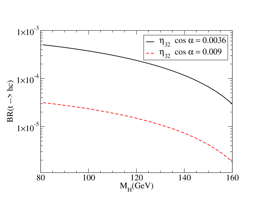
Figure 1: Branching ratio for the rare top decay $t\rightarrow H+c$ for different values of the product of the mixing, $\alpha$, between the lightest Higgs bosons and the additional Higgs boson of the model, and the mixing between the top quark and the charm quark, $\eta_{{\scriptscriptstyle 32}}$. This figure shows that there is a lot of room for future collider experiments either to detect, or to set bounds on this parameters.

The branching ratio for this decay is obtained as the ratio of Eq. (28) to the total width for the top quark, namely

$$\begin{array}[]{c}B(t\rightarrow H^{0}+c)=\frac{\Gamma(t\rightarrow H^{0}+c)}{\Gamma(t\rightarrow b+W)}.\end{array}$$ (29)

Thanks to the possible combined effect of a big $\cos\alpha$ (null mixing between the SM Higgs boson and the additional Higgs bosons) and a big value of $\eta_{{\scriptscriptstyle 32}}$ this branching ratio could be as high as $\approx 3\times 10^{-4}$, for a Higgs mass of 117 $GeV$ as is illustrated in Fig. 1. Perhaps is more realistic to consider the more stringent constraint $\eta_{{\scriptscriptstyle 32}}=0.009$, but even in this case, for $\cos\alpha\approx 1$ there is still sensitivity for detecting a positive signal of order $10^{-5}$ as is shown in same Fig. 1.

III.3 The decay $H^{0}\rightarrow t+\bar{c}$

Finally we also consider the case of a Standard Higgs with a large mass. The best-fit value of the expected Higgs mass, including the new average for the mass of the top quark, is 117 GeV Abazov:2004cs and the upper bound is $M_{H}\leq 251$ GeV at 95 % C L. However, the error for the Higgs boson mass from this global fit is asymmetric, and a Higgs mass of $400$ GeV is well inside the $3\sigma$ region as can be seen in Ref Abazov:2004cs .

We estimate the branching ratio for the decay $H^{0}\rightarrow t+\bar{c}$, where $H^{0}$ is the light neutral Higgs boson of the ALRM. The expression for the partial width is

$$\begin{array}[]{c}\displaystyle\Gamma(H^{0}\rightarrow t+\bar{c})=\\[14.22636pt] \displaystyle\frac{3\,G_{{\scriptscriptstyle F}}\,m_{t}^{2}\,\eta^{2}_{{\scriptscriptstyle 32}}\,\cos^{2}\alpha}{8\,\sqrt{2}\,\pi\,M_{{\scriptscriptstyle H}}^{3}}\,\Big{(}M_{{\scriptscriptstyle H}}^{2}-m_{t}^{2}-m_{c}^{2}\Big{)}\Big{[}\Big{(}M_{{\scriptscriptstyle H}}^{2}-\Big{(}m_{t}+m_{c}\Big{)}^{2}\,\Big{)}\Big{(}M_{{\scriptscriptstyle H}}^{2}-\Big{(}m_{c}-m_{t}\Big{)}^{2}\,\Big{)}\Big{]}^{\frac{1}{2}}.\end{array}$$ (30)

The branching ratio for this decay is obtained as the ratio of Eq. (30) to the total width of the Higgs boson, which will include the dominant modes $H^{0}\rightarrow b+\bar{b}$, $H^{0}\rightarrow c+\bar{c}$, $H^{0}\rightarrow\tau+\bar{\tau}$, $H^{0}\rightarrow W+W$, and $H^{0}\rightarrow Z+Z$. The expressions for these decay widths in the ALRM are:

$$\begin{array}[]{c}\displaystyle\Gamma(H^{0}\rightarrow f+\bar{f})=C_{f}\,\frac{G_{F}\,m^{2}_{f}\,M_{H}\,\eta^{2}_{{\scriptscriptstyle ff}}\,\cos^{2}\alpha}{4\sqrt{2}\,\pi}(1-4\lambda_{f})^{\frac{3}{2}}\end{array}$$ (31)

where $\lambda_{f}=(\frac{m_{f}}{M_{H}})^{2}$, $C_{f}$ = 1 for leptons and $C_{f}$ = 3 for quarks,

$$\begin{array}[]{c}\displaystyle\Gamma(H^{0}\rightarrow W+W)=\frac{G_{F}\,M_{H}^{3}\,\cos^{2}\alpha}{8\sqrt{2}\,\pi}(1-4\lambda_{W})^{\frac{1}{2}}(1-4\lambda_{W}+12\lambda_{W}^{2}),\end{array}$$ (32)

with $\lambda_{W}$ = $(\frac{M_{W}}{M_{H}})^{2}$, and

$$\begin{array}[]{c}\displaystyle\Gamma(H^{0}\rightarrow Z+Z)=\frac{G_{F}\,M_{H}^{3}\,M_{W}^{4}\,X^{2}\,\cos^{2}\alpha}{16\sqrt{2}\,\pi\,M^{4}_{Z}}(1-4\lambda_{Z})^{\frac{1}{2}}(1-4\lambda_{Z}+12\lambda_{Z}^{2}),\end{array}$$ (33)

with $\lambda_{Z}$ = $(\frac{M_{Z}}{M_{H}})^{2}$ and $X$ = $(c_{\theta_{{\scriptscriptstyle W}}}c_{\Theta}-\frac{s_{\theta_{{\scriptscriptstyle W}}}}{r_{\theta_{{\scriptscriptstyle W}}}}t_{\theta_{{\scriptscriptstyle W}}}(s_{\Theta}-r_{\theta_{{\scriptscriptstyle W}}}c_{\Theta}))^{2}$.

We show in Fig. 2 the branching ratios for different decay modes, both for the Standard Model case ($\eta_{{\scriptscriptstyle 32}}=0$ and $\eta_{ii}=1$) and for the FCNC case. We can see that, also for a heavy Higgs, there are chances to either detect or to constrain the mixing angle parameter $\eta_{{\scriptscriptstyle 32}}$. In this case, since all the partial widths have the same dependence on $\cos^{2}\alpha$, the branching ratios will depend only on $\eta_{{\scriptscriptstyle 32}}$.

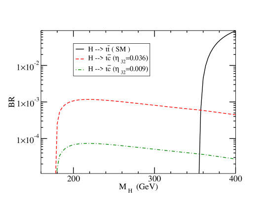
Figure 2: Branching ratio for the rare Higgs decay $H\rightarrow t+\bar{c}$, for different values of $\eta_{{\scriptscriptstyle 32}}$ as a function of the Higgs mass. The standard Higgs decay $H\rightarrow t+\bar{t}$ is also shown.

IV Results and conclusions

We have seen that the ALRM allows relatively big values of $\eta_{{\scriptscriptstyle 32}}$. The $t\to H+c$ branching ratio could be of order of $10^{-4}$, which is at the reach of LHC. For example, it has been estimated that the LHC sensitivity (at 95 % C. L.) for this decay is $Br(t\to Hc)\leq 4.5\times 10^{-5}$ Aguilar-Saavedra:2000aj ; this branching ratio would be obtained in this model for a top-charm mixing $\eta_{{\scriptscriptstyle 32}}=0.015$ and a diagonal ordinary top coupling $\eta_{{\scriptscriptstyle 22}}\simeq 0.98$. On the other hand, the FCNC mode $H\to t+\bar{c}$ may reach a branching ratio of order $10^{-3}$ and can also be a useful channel to look for signals of physics beyond the SM in the LHC.

The ALRM is a well motivated model that rises from different theoretical motivations and has a rich phenomenology. In particular, we have studied the ALRM in the context of rare top decays and we have found that these models could be tested in the next generation of colliders.

References

• (1) V. M. Abazov et al. [D0 Collaboration], Nature 429, 638 (2004) [arXiv:hep-ex/0406031].
• (2) S. Béjar, J. Guasch and J. Solá, Nucl. Phys. B600, 21 (2001).
• (3) J. L. Diaz-Cruz, R. Martinez, M. A. Perez and A. Rosado, Phys. Rev. D41 891 (1990);
• (4) E. Jenkins, Phys. Rev. D56, 458 (1997).
• (5) B. Mele, S. Petrarca, A. Soddu, Phys. Lett. B435, 401 (1998).
• (6) G. Eilam, J. L. Hewett and A. Soni, Phys. Rev. D44, 1473 (1991).
• (7) J. A. Aguilar-Saavedra and B. M. Nobre, Phys. Lett. B553 251 (2003).
• (8) G. Eilam, J. L. Hewett and A. Soni, Phys. Rev. D59, 039901(E) (1999), Erratum.
• (9) A. M. Curiel, M. J. Herrero and D. Temes, Phys. Rev. D67, 075008 (2003).
• (10) T. Han, R. D. Peccei and X. Zhang, Nuc. Phys. B454 527 (1995); T. Han, K. Whisnant, B. L. Young and X. Zhang, Phys. Rev. D55 7241 (1997) [arXiv:hep-ph/9603247]; F. del Aguila and J. A. Aguilar-Saavedra, Phys. Lett. B462 310 (1999); J. L. Díaz-Cruz, M. A. Pérez, G. Tavares-Velasco and J. J. Toscano, Physical Review D60 115014 (1999); F. del Aguila and J. A. Aguilar-Saavedra, Nuc. Phys. B576 56 (2000); C. x. Yue, G. r. Lu, Q. j. Xu, G. l. Liu and G. p. Gao, Phys. Lett. B508 290 (2001); J. Cao, Z. Xiong and J. M. Yang, Phys. Rev. D 67 071701(R) (2003); Nuc. Phys. B651 87 (2003) A. Cordero-Cid, M. A. Perez, G. Tavares-Velasco and J. J. Toscano, hep-ph/0407127. J. L. Díaz-Cruz, Hong-Jian He, C. P. Yuan, Phys. Lett. B530 179 (2002).
• (11) J. A. Aguilar-Saavedra, Phys. Rev. D67 035003 (2003) [Erratum Phys. Rev. D69 099901 (2004)]
• (12) J. L. Díaz Cruz, D. A. López Falcón, Phys. Rev. D61 051701(R) (2000); P. Fernández de Córdoba, R. Gaitán Lozano, A. Hernández-Galeana and J. M. Rivera-Rebolledo, Rev. Mex. Fis. 50 239 (2004).
• (13) H. P. Nilles, Phys. Rept. 110 1 (1984); H. E. Haber, G. L. Kane, Phys. Rept. 117 75 (1985); W. S. Hou, Phys. Lett. B296 179 (1992); D. A. Demir, Phys. Lett. B571 193 (2003); A. Brignole and A. Rossi, Phys. Lett. B566 217 (2003);
• (14) S. Béjar, J. Guasch and J. Solá, Nuc. Phys. B675 270 (2003).
• (15) M. Beneke, I. Efthymiopoulos, M. L. Mangano, J. Womerslwy et. al., hep-ph/0003033.
• (16) J. C. Pati and A. Salam Phys. Rev. D10 275 (1974); R. N. Mohapatra and J. C. Pati Phys. Rev. D11 566 (1975) and Phys. Rev. D11 2558 (1975); G. Senjanovic and R. N. Mohapatra Phys. Rev. D12 1502 (1975);
• (17) Rabindra N. Mohapatra Unification and Supersymmetry Springer 2003 and references therein.
• (18) A. Davidson and K. C. Wali, Phys. Rev. Lett. 59 393 (1987); S. Rajpoot Phys. Lett. B191 122 (1987).
• (19) K. Kiers, J. Kolb, J. Lee, A. Soni and G. H. Wu, Phys. Rev. D66 095002 (2002); [arXiv:hep-ph/0205082].
• (20) R. N. Mohapatra Phys. Lett. B201 517 (1988); K. S. Babu, X-G He Mod. Phys. Lett. A4 61 (1989).
• (21) B. S. Balakrishna, Phys. Rev. Lett. 60 1602 (1988); K. S. Babu and R. N. Mohapatra, Phys. Rev. D41 1286 (1990);
• (22) S. M. Barr, D. Chang and G. Senjanovic, Phys. Rev. Lett. 67 2765 (1991).
• (23) V. E. Cerón, U. Cotti, J. L. Díaz-Cruz and M. Maya, Phys. Rev. D57 1934 (1998); U. Cotti et. al. Phys. Rev. D66 015004 (2002).
• (24) P. Langacker and D. London, Phys. Rev. D38 886 (1988).
• (25) J. A. Aguilar-Saavedra, Acta Phys. Pol. B 35 2695 (2004) arXiv:hep-ph/0409342.
• (26) O. Adriani et. al., L3 Coll, Phys. Lett. B306 187 (1993); J. Polak and M. Zralek, Phys. Rev. D46 3871 (1992); M. Maya and O. G. Miranda Z. Phys. C68 481 (1995).
• (27) G. Abbiendi et al. [OPAL Collaboration], Phys. Lett. B521 181 (2001).
• (28) F. del Aguila, J. A. Aguilar-Saavedra, Phys. Rev. Lett. 82 1602 (1999).
• (29) D. Acosta et al, Phys. Rev. Lett. 90 131801 (2003).
• (30) S. Eidelman et al. (Particle Data Group), Phys. Lett. B 592 1 (2004).
• (31) J. A. Aguilar-Saavedra and G. C. Branco, Phys. Lett. B495 347 (2000). [arXiv:hep-ph/0004190].