On the quark-gluon plasma search

Abstract

We report on the effect of the quantum statistics on the two-proton spin correlation (SC) in cold and thermal nuclear matter. We have found that two nucleons SC function can be well approximated by a guassian with correlations length $\sigma\sim 1.2$ fm. We have proposed SC measurement on low protons energy as test of the quark-gluon plasma formation in relativistic heavy ions collisions.

Lattice QCD predict a phase transition from Hadrons gaz (HG) to quark-gluon plasma (QGP) at deconfinement temperature, $T_{d}\sim 170\,$MeV. It is believed that $T_{d}$ has been reached in the relativistic heavy ions collision. Several signatures of the QGP formation have been proposed in the literature. The proposed signatures include:

• Dilepton production;

• Photon production;

• Hanbury-Brown-Twiss Effect;

• Strangeness enhancement;

• $J/\Psi$ suppression.

All this effect have been intensively studied in the literature. For example, strangeness enhancement raf1 has been observed at the SPS energy and recently at RHIC. However, it has been shown that strangeness enhancement can be explained in terms of statistical model formulated in canonical ensemble with respect to strangeness conservation ham2 . This problem also hold for other signatures in the sense that those signatures can be considered as clear indication in the favor of QGP formation but not decisive. Therefore, one may ask the following question: is there exists a signature that shows up only in one phase (QGP or HG) and not in the other one? This will be our goal. In this paper, we propose the spin correlation (SC) measurement as fundamental probe. SC discussed here is due to the indistinguishability of nucleons and the existence of quantum statistic discussed, in different context, in 6 .

It is known that if the QGP is produced in relativistic heavy ions collision a supercooling and sudden hadronization is expected ham3 . Therefore, in this scenario, the hadrons are produced from phase space. Thus, from this point of view, SC due to the quantum statistics will not play a role as the hadrons produced suddenly and escape from the local volume. However, if the hadrons are produced from HG phase they have to respect quantum statistics. Therefore, a possible SC can be expected. To the best of our knowledge, for a non-comprehensible reason, this effect has been rarely studied explicitly in nuclear physics bert1 .

In the next section we aim on the evaluation of the SC function, the quantum, and the classical correlations between two protons inside a nucleus. In section II we will discuss the two-proton SC function in thermal nuclear matter as test of QGP formation. Finally our conclusion is given in section III.

I SC in cold nuclear matter

Fig. 1: The correlation function at $0^{\circ}$ (dotted line), the relative entropy of entanglement (dashed line) and the classical correlations (solid line) are depicted in dependence on $k_{f}r$. Small circles represent our predictions for the nuclear matter where we have used $k_{f}\sim 1.27\,{\rm fm}^{-1}$ and $r\sim 1.2$ fm.. The large dashed line represent the gaussian approximation of the mixing parameter.

In this section, we will evaluate the correlations between two nucleons (protons or neutrons) in Fermi sea approach to nuclear matter 101 ; 100 . Therefore, in the coordinate representation, the density matrix elements of two nucleons are

$$\langle\Psi_{0}|\psi^{{\dagger}}_{\sigma_{2}^{\prime}\bf r_{2}^{\prime}}\psi^{{\dagger}}_{\sigma_{1}^{\prime}\bf r_{1}^{\prime}}\psi_{\sigma_{2}\bf r_{2}}\psi_{\sigma_{1}\bf r_{1}}|\Psi_{0}\rangle\,,$$ (1)

where $\psi_{\sigma\bf r}=\frac{1}{V}\sum_{\bf k}e^{i\bf k\cdot r}a_{\sigma\bf k}$ and $|\Psi_{0}\rangle=\prod_{|k|\leq k_{f}}a^{{\dagger}}_{\sigma\bf k}|0\rangle\,$ is the ground state of the system. As usual, in the continuum limits $[a^{{\dagger}}_{\sigma\bf k},a_{\sigma^{\prime}\bf k^{\prime}}]=\delta_{\sigma\sigma^{\prime}}\delta({\bf k-k^{\prime}})$.

A straightforward calculations gives the explicit form of the two-particle space-spin density matrix 99

$$\rho^{sp} = \frac{1}{2}\left(F({\bf r_{1}-r_{1}^{\prime}})F({\bf r_{2}-r_{2}^{\prime}})\delta_{\sigma_{1}\sigma_{1}^{\prime}}\delta_{\sigma_{2}\sigma_{2}^{\prime}}\right.$$ (2)

$$\left.-F({\bf r_{1}-r_{2}^{\prime}})F({\bf r_{2}-r_{1}^{\prime}})\delta_{\sigma_{1}\sigma_{2}^{\prime}}\delta_{\sigma_{2}\sigma_{1}^{\prime}}\right)\,$$

with $F({\bf r})=\frac{1}{V}\sum_{\bf k}e^{i\bf k\cdot r}$. Depending on the space density matrix, two spins may be entangled. We obtain Vedral’s result 6 only if ${\bf r_{1}=r_{1}^{\prime}}$ and ${\bf r_{2}=r_{2}^{\prime}}$, that is, only diagonal elements of a space density matrix are considered. The two-spin density matrix, depending on the relative distance between two nucleons $r=|{\bf r_{1}-r_{2}}|$, reads

$$\rho^{s}=\frac{1}{4-2f^{2}}\left(\begin{array}[]{cccc}1-f^{2}&0&0&0\\ 0&1&-f^{2}&0\\ 0&-f^{2}&1&0\\ 0&0&0&1-f^{2}\end{array}\right)\,,$$ (7)

$f(r)=3j_{1}(k_{f}r)/k_{f}r$ and $j_{1}$ is the spherical Bessel function. We find that $\rho^{s}$ is a Werner state characterized by a single parameter $p=f^{2}/(2-f^{2})$.

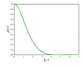
Fig. 2: The mixing parameter $p(r)$ at $T=0$ (solid line) and for $T=0.2\mu_{B}$ (dashed line).

In Fig. 1 we show as function of $k_{f}r$ the correlation function at $0^{\circ}$ ham4

$$P(\theta)={N_{++}+N_{--}-N_{+-}-N_{-+}\over N_{total}}=p\cos(\theta)\,,$$ (8)

($\theta$ is the angle between the quantization axis and $+$ and $-$ represent the positive and negative spin projection on the quantization axis) and the relative entropy of entanglement Vedr97 ,

$$E_{r}=\min_{\rho^{*}\in{\cal D}}S(\rho\|\rho^{*})\,,$$ (9)

where ${\cal D}$ is a set of all separable states in the Hilbert space in which $\rho$ is defined. Also shown in Fig. 1 the classical correlations Hami03 ,

$$\Psi(\rho)=S(\rho\|\rho_{A}\otimes\rho_{B})-\min_{\rho^{*}\in{\cal D}}S(\rho\|\rho^{*})\,,$$ (10)

where $\rho_{A}$ and $\rho_{B}$ are the reduced density matrices. The small circles in Fig. 1 represent our predictions for the nuclear matter with typical values of $k_{f}\sim 1.27\,{\rm fm}^{-1}$ and $r\sim 1.2$ fm 100 ; 101 . We observe that the mixing parameter, $p(r)=P(0^{\circ})$, can be approximated with a gaussian function

$$p(r)=e^{-r^{2}/2\sigma^{2}}\,,$$ (11)

with $\sigma=1.2$ fm, see Fig. 1.

The mixing parameter, $p(r)$, can be measured experimentally. In fact, following Bertulani approach bert1 for weakly bound nucleons as in $\rm{}^{1}H(^{6}He,^{2}He)^{5}H$ reaction one can argue, using our results, that the relative energy distribution of the two outgoing proton $\rm{}^{2}He$ without the final state interaction should reads

$$\sigma(E_{pp})\propto\sqrt{E_{pp}}\left(1+e^{-R^{2}/2\sigma^{2}}[\cos(\sqrt{m_{n}E_{pp}/\hbar^{2}}R)]\right)\,,$$ (12)

where $E_{pp}$ is the relative energy between the two protons and $R$ is the size of the source region. Therefore, from experimental data kors1 we can extract the mixing parameter $p(r)$ hami3 . Also our mixing parameter can be extracted from coulomb dissociation of $\rm{}^{11}Li$ simo1 see forthcoming paper hami3 .

II SC in thermal nuclear matter

For simplicity we will only consider protons from the all known particles and resonances of HG. The formulation described in the above section can be applied in this case. However, at finite temperature the occupation probability of state ${\bf k}$ is the Fermi Dirac distribution $n_{\bf k}=(1+e^{\beta(\epsilon_{\bf k}-\mu_{B})})^{-1}$. As results the function $f(r)$ should be replaced by:

$$f(r)=2\frac{\sum_{\bf k}n_{\bf k}e^{i\bf k\cdot r}}{\sum_{\bf k}n_{\bf k}}.$$ (13)

From the last section we know that $P(0^{\circ})=p=f^{2}/(2-f^{2})$. Thus, in order to find the correlations function, we need an estimation of $f$. Because, the thermal freeze out temperature is $T_{th}\sim 100$MeV well below the baryonic chemical potential $\mu_{B}\sim 266$ MeV stac1 , the correlation function can be approximated by $p(r,T=0)$ as it can be seen in Fig. 2. However, with this conditions $k_{f}\sim 10\,\rm fm^{-1}$, thus the correlation function is zero. Nevertheless, we can still have correlation if we consider only the outgoing proton with momentum $\rm<2\,fm^{-1}$ which produce a large amount of correlation $\sim 0.25$ that can be measured experimentally. For example, in 158 AGeV Pb–Pb collisions at SPS, assuming Bjorken scaling at the central rapidity with $\Delta y\sim 0.2$, the longitudinal dimension of the volume is $d=\Delta y\,\tau\sim 2\,$fm. Thus, SC can be performed on those protons. A carbon analyzer as in ham4 is suitable for this analysis.

Moreover, our results can have effect on the two proton Hanbury-Brown-Twiss (HBT) interferometery. In fact, it is known that the two-proton correlation function is influenced by identical particle interference, short-range hadronic interaction, and long-range Coulomb repulsion. For noninteracting identical particles, the squared wave function has the form

$$\Psi^{2}({\bf q,r})\propto 1\pm\cos({2\bf qr})\,,$$ (14)

where the plus sign stands for singlet spin state and minus sign for triplet. In the literature two assumption are frequently used wolf1

• spin parallel orientations (triplet) or,

• random spin orientations.

Clearly from the discussion above the situation can be different and contribution from singlet state can dominate for small frequency hami3 . This effect can be seen in HBT interferometery by considering large relative energy in order to reduce the final state interaction na491 ; hami3 .

III Conclusion

In this paper, we have proposed two-proton spin correlation measurement as potential test of the quark-gluon plasma formation in relativistic heavy ions collisions. We have found that a non negligible correlation can be measured experimentally for protons with momentum $\rm<2\,fm^{-1}$. A more detailed calculations will be addressed in the near future.

References

- (1) J. Rafelski, and B. Muller, Phys Rev Lett 48, 1066, (1982)
- (2) S. Hamieh, K. Redlich, and A. Tounsi, Phys.Lett. B 486, 61, (2000)
- (3) V. Vedral, Central Eur.J.Phys.1, 289 (2003).
- (4) C. Bertulani, J. Phys. G 29, 769, (2003)
- (5) S. Hamieh, J. Letessier, and J. Rafelski, Phys.Rev. C 62, 064901, (2000)
- (6) C. N. Yang, Rev. Mod. Phys. 34, 694 (1962)
- (7) V. Vedral, et al.,Phys. Rev. Lett. 78, 2275 (1997)
- (8) S. Hamieh, et al., Phys. Rev. A 67, 014301 (2003)
- (9) Shell model and optical potential suggest that, to a first approximation, we may picture the nucleus as potential well with 42 MeV deep and filed up to about 8 MeV below the top. Thus, and fm.
- (10) Similar calculations can be made in Shell model.
- (11) A. Korsheninnikov et. al, Phys. Rev. Lett. 87, 092501 (2002)
- (12) S. Hamieh, in preparation
- (13) H. Simon, et al., Phys. Rev. Lett. 83, 496 (1999)
- (14) P. Braun-Munzinger, I. Heppe, and J. Stachel, Phys.Lett. B 465, 15, (1999)
- (15) S. Hamieh, et al., J. Phys. G 30, 481, (2004)
- (16) W. Bauer, and C. Gelbke, Annu. Rev. Nucl. Part. Sci. 42, 77, (1992)
- (17) NA49 Collaboration, Phys. Lett. B 467, 21, (1999)