$\rho^{0}$ mass in a hot hadron gas

Abstract

We study the behavior of the $\rho^{0}$ vector mass during the hadronic phase of an ultra-relativistic heavy-ion collision at finite temperature. We show that scattering with the most abundant particles during this stage, namely, pions, kaons and nucleons, leads to an overall temperature dependent, decrease of the $\rho^{0}$ intrinsic mass at rest, compared to its value in vacuum. The main contributions arise from $s$-channel scattering with pions through the formation of $a_{1}$ resonances as well as with nucleons through the formation of even parity, spin 3/2 [N(1720)] and 5/2 [$\Delta$(1905)] nucleon resonances. We show that it is possible to achieve a shift in the intrinsic $\rho^{0}$ mass of order $\sim-40$ MeV, when including the contributions of all the relevant mesons and baryons that take part in the scattering, for temperatures between chemical and kinetic freeze-out.

I Introduction

The $\rho$ vector meson plays a special role in ultra-relativistic heavy-ion collisions since its vacuum life time ($\sim 1.3$ fm) is shorter than the life time of the system created in the reaction. Therefore, any changes in the properties of this meson are expected to comprise information about the conditions of the collision at the time when the meson decayed. This expectation is at the core of the intensive studies, both experimental experiments and theoretical Models regarding the $\rho$ electromagnetic decay channels.

The advent of large multiplicity events at RHIC energies has allowed to also study the $\rho$ decay into pions, which is by far the most important of its decay channels. A remarkable result reported by the STAR collaboration is a shift of $\sim-40$ MeV and $\sim-70$ MeV for the peak of the invariant mass distribution of the decay $\rho^{0}\rightarrow\pi^{+}\pi^{-}$ in minimum bias p + p and peripheral Au + Au collisions, respectively, at $\sqrt{s_{NN}}=200$ GeV as compared to the vacuum value STAR .

A plausible interpretation of the above result, as regards to the heavy-ion environment, is that one is in fact looking at the medium induced modifications of the meson driven by its decay, regeneration and ree-scattering within a hadronic system over a short interval of time, namely, the last stage of the collision, between chemical and kinetic freeze out, lasting a time interval of the order of the life time of the meson. The fact that the resonance spectral density can be experimentally reconstructed means that the hadronic system is dilute enough so that the decay products do not suffer significant ree-scattering after being produced.

In order to describe medium induced modifications to the intrinsic properties (mass and width) of a hadronic resonance such as $\rho$, it is necessary to resort to effective Lagrangians representing the interactions of the resonance with the rest of the hadronic matter in the environment. Based on general grounds, these Lagrangians are built to respect the basic symmetries of the strong interaction, among them, current conservation and parity invariance. Thermal modifications to the $\rho$ intrinsic properties are computed by evaluating the one-loop modification of its self-energy. Attention is paid to those hadrons whose rest mass is near the threshold for $s$ or $t$ channel resonance formation and with a sizable coupling to $\rho$ and to the most abundant particles in the hadronic phase of the collision, namely pions/kaons and nucleons. The phenomenological coupling constants are evaluated by comparing the model prediction of the vacuum decay rate, into the given channel, with the experimentally measured branching ratio.

Temperature driven modifications to intrinsic properties of $\rho$ have been thoroughly worked out from interactions with mesons Rapp when considering only scattering in the $s$-channel. The case of interactions with baryons has mainly been studied in connection with changes caused by dense nuclear matter effects (see however Refs. Rapp3 ) and by means of non-relativistic approximations for the interaction Lagrangians Teodorescu ; Friman ; Peters . In a recent work acm interactions of $\rho$ with baryon resonances have been considered in a relativistic framework. When including also the contributions from scattering off various meson resonances, it has been shown that the intrinsic $\rho$ mass at rest decreases with increasing temperature.

The purpose of this work is to give full account of the thermal modifications to the mass of the $\rho^{0}$ meson when considering its scattering off pions/kaons and nucleons in a thermalized hadronic medium, such as the one that is expected to be produced during the dilute, almost baryon free, last stage of an ultra-relativistic heavy-ion collision. In particular we show how a systematic thermal field-theoretical calculation of the real part of the one-loop $\rho$ self-energy yields the total contribution, both form $s$- and $t$-channel resonance exchanges, to the thermal mass of $\rho$ at rest. We find that $\rho$ scattering off pions through the exchange of pions themselves significantly contributes to an increase of the $\rho$ thermal mass. However, when considering also the contribution from scattering off pions through the exchange of pseudo-vector resonances, in particular $a_{1}$, and off nucleons through the exchange of various baryonic resonances, in particular N(1720) and $\Delta(1905)$, the overall result is a decrease of the thermal $\rho$ mass at rest.

To describe all the interactions of $\rho$ we work within a full relativistic formalism, making use of the generalized Rarita-Schwinger propagators for fermion fields with spin higher than 1/2. We work in the imaginary-time formulation of thermal field theory to compute the one-loop $\rho$ self-energy $\Pi_{\mu\nu}$, when interacting with the relevant hadrons.

The work is organized as follows: In Sec. II we review essentials of the computation of the real part of the one-loop thermal self-energy of a particle in a scalar model, separating explicitly its $s$- and $t$-channel contributions. In Sec. III we compute the contribution to the $\rho^{0}$ thermal mass from interactions with nucleons and baryon resonances. We also compute the coupling constants used in the calculation comparing the theoretical expression for the branching ratio into the $\rho$ nucleon channel with the experimentally measured value. In Sec. IV we compute the contribution to the $\rho^{0}$ thermal mass from interactions with pions and kaons and various other meson resonances. In Sec. V put together the above contributions to compute the behavior of the $\rho^{0}$ mass at rest with temperature. Finally, we summarize our results and conclude in Sec. VI.

II Thermal self-energy in a scalar theory

Recall that the self-energy $\Pi$ is related to the intrinsic $\rho$ properties by ${\mbox{Im}}\ \Pi=-M_{\rho}\Gamma^{\mbox{\tiny{tot}}}$, $M_{\rho}=\sqrt{m_{\rho}^{2}+{\mbox{Re}}\ \Pi}$, where $m_{\rho}$ is the mass of $\rho$ in vacuum, $M_{\rho}$ and $\Gamma^{\mbox{\tiny{tot}}}$ are the (temperature and/or density dependent) intrinsic mass and total decay width of the $\rho$ meson, respectively and ${\mbox{Re}}\ \Pi$ and ${\mbox{Im}}\ \Pi$ represent the real and imaginary parts of $\Pi$, respectively.

The real part of the one-loop $\rho$ self-energy receives contributions stemming from the various particles (fermions or bosons) in the loop interacting with $\rho$. Depending on the Lorentz nature of the interacting particles, the tensor structure of the self-energy can become very cumbersome and difficult to keep track of. Nevertheless, the analytic structure of the induced changes to the mass of $\rho$ at finite temperature can already be understood in a simpler scalar theory. Let us therefore here look at such case.

Consider the one-loop Feynman diagram depicted in Fig. 1 representing the self energy of a scalar field $\Phi$ interacting with other two scalar fields $\phi_{1}$ and $\phi_{2}$ through the interaction Lagrangian

$${\mathcal{L}}_{I}=-{\mbox{g}}\Phi\phi_{1}\phi_{2}\,,$$ (1)

where g is the coupling constant with dimensions of energy. Field $\Phi$ has mass $Q^{2}=q_{0}^{2}-q^{2}=M^{2}$ whereas fields $\phi_{1}$ and $\phi_{2}$ have masses $m_{1}$ and $m_{2}$, respectively. Without lose of generality, let us take $m_{2}>m_{1}$.

Figure 1: One-loop self-energy Feynman diagram representing the interaction of a scalar particle $\Phi$ with two other scalar particles $\phi_{1}$ and $\phi_{2}$.

In the imaginary-time formalism of thermal field theory, the self-energy diagram of Fig. 1 can be expressed, after performing the sum over the Matsubara frequencies, as LeBellac

$$\Pi(i\omega,q) = -{\mbox{g}}^{2}\int\frac{d^{3}k}{(2\pi)^{3}}\frac{1}{4E_{1}E_{2}}\Big{\{}\left[1+n(E_{1})+n(E_{2})\right]$$ (2)

$$\left(\frac{1}{i\omega-E_{1}-E_{2}}-\frac{1}{i\omega+E_{1}+E_{2}}\right)$$

$$- \left[n(E_{1})-n(E_{2})\right]$$

$$\left(\frac{1}{i\omega-E_{1}+E_{2}}-\frac{1}{i\omega+E_{1}-E_{2}}\right)\Big{\}}\,,$$

where $E_{1}=\sqrt{k^{2}+m_{1}^{2}}$, $E_{2}=\sqrt{({\mathbf{q}}-{\mathbf{k}})^{2}+m_{2}^{2}}$ and

$$n(x)=\frac{1}{e^{\beta x}-1}\,,$$ (3)

is the Bose-Einstein distribution with $1/\beta=T$ being the temperature.

The retarded self-energy is obtained by means of the analytic continuation $i\omega\rightarrow q_{0}+i\epsilon$. In this manner, the real and imaginary parts of the retarded self-energy are given by

$$\!\!\!\!\!{\mbox{Re}}\ \Pi(q_{0},q) \!\!\!\!\!\!\!\!\!\!=\!\!\!\!\!\!\!\!\!\! -{\mbox{g}}^{2}{\mathcal{P}}\int\frac{d^{3}k}{(2\pi)^{3}}\frac{1}{4E_{1}E_{2}}$$

$$\Big{\{}\left[1+n(E_{1})+n(E_{2})\right]$$

$$\left(\frac{1}{q_{0}-E_{1}-E_{2}}-\frac{1}{q_{0}+E_{1}+E_{2}}\right)$$

$$\!\!\!\!\!\!\!\!\!\!-\!\!\!\!\!\!\!\!\!\! \left[n(E_{1})-n(E_{2})\right]$$

$$\left(\frac{1}{q_{0}-E_{1}+E_{2}}-\frac{1}{q_{0}+E_{1}-E_{2}}\right)\Big{\}}\,,$$

$$\!\!\!\!\!{\mbox{Im}}\ \Pi(q_{0},q) = \pi{\mbox{g}}^{2}\int\frac{d^{3}k}{(2\pi)^{3}}\frac{1}{4E_{1}E_{2}}$$ (4)

$$\Big{\{}\left[1+n(E_{1})+n(E_{2})\right]$$

$$\left(\delta(q_{0}-E_{1}-E_{2})-\delta(q_{0}+E_{1}+E_{2})\right)$$

$$\!\!\!\!\!\!\!\!\!\!-\!\!\!\!\!\!\!\!\!\! \left[n(E_{1})-n(E_{2})\right]$$

$$\left(\delta(q_{0}-E_{1}+E_{2})-\delta(q_{0}+E_{1}-E_{2})\right)\!\!\!\Big{\}}$$

where ${\mathcal{P}}$ represents the Cauchy principal value. Notice that the first and second of Eqs. (4) are related by a dispersion relation without subtractions.

Let us concentrate in the first of Eqs. (4) and consider the limit ${\mathbf{q}}=0$, that is, the situation when the particle $\Phi$ is at rest. Furthermore, let us look only at the temperature dependent terms. We can then write

$${\mbox{Re}}\ \Pi(q_{0},q) \rightarrow -{\mbox{g}}^{2}{\mathcal{P}}\int\frac{d^{3}k}{(2\pi)^{3}}\frac{1}{4E_{1}E_{2}}$$ (5)

$$\Big{\{}n(E_{1})\left[\frac{1}{q_{0}-E_{1}-E_{2}}-\frac{1}{q_{0}-E_{1}+E_{2}}\right.$$

$$+ \left.\frac{1}{q_{0}+E_{1}-E_{2}}-\frac{1}{q_{0}+E_{1}+E_{2}}\right]$$

$$+ n(E_{2})\left[\frac{1}{q_{0}-E_{2}-E_{1}}-\frac{1}{q_{0}-E_{2}+E_{1}}\right.$$

$$+ \left.\frac{1}{q_{0}+E_{2}-E_{1}}-\frac{1}{q_{0}+E_{2}+E_{1}}\right]\Big{\}}\,,$$

where $E_{i}=\sqrt{k^{2}+m_{i}^{2}}$, ($i=1,2$). $E_{1}$ and $E_{2}$ are related by $E_{2}^{2}=E_{1}^{2}+m_{2}^{2}-m_{1}^{2}$. Notice that the coefficient of $n(E_{2})$ in Eq. (5) is obtained from the coefficient of $n(E_{1})$ by the exchange $E_{2}\leftrightarrow E_{1}$.

Figure 2: Two of the Feynman diagrams obtained by computing the real part of the one-loop self-energy of $\Phi$ representing (i) $t$-channel and (ii) $s$-channel scattering of particle $\Phi$ off particle $\phi_{1}$ with the exchange of particle $\phi_{2}$.

For the case at hand, namely $m_{2}>m_{1}$, the terms proportional to $n(E_{2})$ are suppressed with respect to those proportional to $n(E_{1})$, thus, for the ease of the discussion let us for the time being ignore the former. After the change of integration variable $k\rightarrow E_{1}=\sqrt{k^{2}+m_{1}^{2}}$ in Eq. (5) one gets

$${\mbox{Re}}\ \Pi(q_{0},q=0) = -\frac{{\mbox{g}}^{2}}{(2\pi)^{2}}\frac{1}{2q_{0}}{\mathcal{P}}\int_{m_{1}}^{\infty}dE_{1}\sqrt{E_{1}^{2}-m_{1}^{2}}$$ (6)

$$n(E_{1})\Big{\{}\frac{-1}{E_{1}-\left[\frac{q_{0}^{2}-(m_{2}^{2}-m_{1}^{2})}{2q_{0}}\right]}$$

$$+ \frac{1}{E_{1}+\left[\frac{q_{0}^{2}-(m_{2}^{2}-m_{1}^{2})}{2q_{0}}\right]}\Big{\}}\,.$$

For definitiveness, take $q_{0}>0$. Also define

$$a\equiv\frac{q_{0}^{2}-(m_{2}^{2}-m_{1}^{2})}{2q_{0}}\,.$$ (7)

The integrand in Eq. (7) is singular for $q_{0}=\pm a$ when $a\geq m_{1}$. We therefore have two instances for the integrand to become singular:

(i) $a>0$, this means that $q_{0}>\sqrt{m_{2}^{2}-m_{1}^{2}}$ and thus there are singularities for $q_{0}\geq m_{1}+m_{2}$.

(ii) $a<0$, this means that $0<q_{0}<\sqrt{m_{2}^{2}-m_{1}^{2}}$ and thus that there are singularities for $0\leq q_{0}\leq m_{2}-m_{1}$.

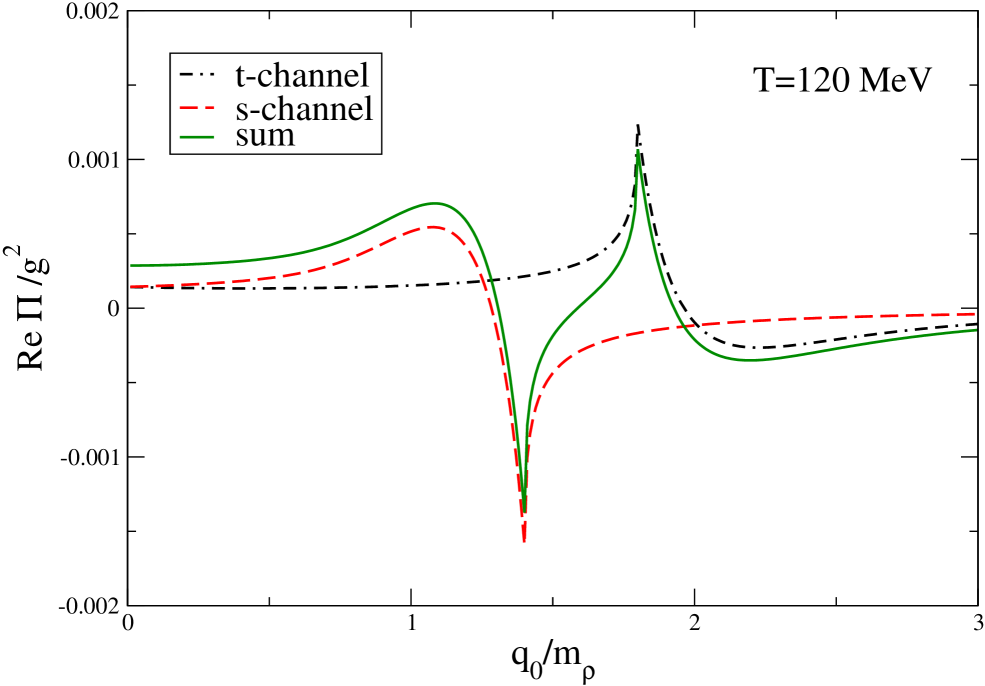
Figure 3: Real part of the one-loop self-energy for particle $\Phi$ scaled to the square of the dimension-full coupling constant g in the scalar model showing the $t$- and $s$-channel contributions, separate and combined. For this example we have taken $m_{1}=0.2m_{\rho}$, $m_{2}=1.6m_{\rho}$ and $T=120$ MeV. Notice that the $s$-channel contribution is maximum in magnitude at $M=q_{0}=m_{2}-m_{1}$ whereas the $t$-channel contribution is maximum in magnitude at $M=q_{0}=m_{2}+m_{1}$. For other values of $q_{0}$, these contributions are of similar magnitude showing the importance to account for both of them in the computation of $\Pi$.

The term in Eq. (6) with singularity for $a>0$ (the first term) corresponds to the probability associated to $t$-channel scattering of particle $\Phi$ off particle $\phi_{1}$ with the interchange of particle $\phi_{2}$ as depicted in Fig. 2(i). Similarly, the term in Eq. (6) with singularity for $a<0$ (the second term) corresponds to $s$-channel scattering of particle $\Phi$ off particle $\phi_{1}$ with the interchange of particle $\phi_{2}$ as depicted in Fig. 2(ii). These are the two possibilities that one obtains when cutting the intermediate line associated with particle $\phi_{1}$ in the self energy diagram of Fig. 1, as corresponds to the calculation of the real part of $\Pi$.

Figure 3 shows the contributions to ${\mbox{Re}}\ \Pi(q_{0},q=0)$ corresponding to $t$- and $s$-channel scattering, separate and combined. Notice that both contributions are of the same magnitude except when $q_{0}\simeq m_{1}+m_{2}$ where the $t$-channel dominates or when $q_{0}\simeq m_{2}-m_{1}$ where the $s$-channel dominates. At these values of $q_{0}$ the integral has cusps but it is otherwise finite since it corresponds to the Cauchy principal value.

The above calculation outlines the basic features of the one-loop real part of the self-energy of a given particle in interaction with other two as a function of its mass at rest. In the following sections we will carry out similar considerations for the Lagrangians corresponding to interactions of $\rho$ with several hadrons at finite temperature, where details concerning the strength of the specific interaction will differ but otherwise the above general features will remain.

$R$	$J^{P}$	$\Gamma^{\mbox{\tiny{vac}}}_{R\rightarrow\rho N}{\mbox{(MeV)}}$	$\Gamma^{\mbox{\tiny{vac}}}_{\mbox{\tiny{tot}}}{\mbox{(MeV)}}$	$f_{J^{P}}$	$f_{J^{P}}^{\mbox{\tiny{N--R}}}$
$N$(1520)	$3/2^{-}$	$25$	120	$9.7$	$7$
$N$(1720)	$3/2^{+}$	$100$	150	$7$	$7.8$
$\Delta$(1700)	$3/2^{-}$	$120$	300	$4.4$	$5$
$\Delta$(1905)	$5/2^{+}$	$210$	350	$12.9$	$12.2$

Table 1: List of baryon resonances included in the calculation. The last column corresponds to the values of the coupling constants for a non-relativistic (N-R) calculation as computed in Ref. Peters .

III Interactions of $\rho$ with nucleons and baryon resonances

III.1 Self-energy

A look at the review of particle physics Hagiwara reveals the existence of four baryon resonances with rest masses near the sum of the rest masses of $\rho$ and nucleon ($N$), where, as we have seen in Sec. II, we could expect an important contribution to the thermal modification of the $\rho$ mass. These have also sizable decay rates into the $\rho-N$ channel. The resonances are N(1520), N(1720), $\Delta$(1700) and $\Delta$(1905). Table I shows their quantum numbers and branching ratios into the $\rho-N$ channel.

The interaction Lagrangians ${\mathcal{L}}$ are given by

$${\mathcal{L}}=\left\{\begin{array}[]{lr}\frac{f_{3/2^{-}}}{m_{\rho}}{\mathcal{F}}_{\rho N3/2^{-}}\bar{\psi}^{\mu}\gamma^{\nu}\psi F_{\mu\nu}&\left(\ J^{P}=\frac{3}{2}^{-}\right)\\ \frac{f_{3/2^{+}}}{m_{\rho}}{\mathcal{F}}_{\rho N3/2^{+}}\bar{\psi}^{\mu}\gamma^{5}\gamma^{\nu}\psi F_{\mu\nu}&\left(\ J^{P}=\frac{3}{2}^{+}\right)\\ \frac{f_{5/2^{+}}}{m_{\rho}^{2}}{\mathcal{F}}_{\rho N5/2^{+}}\bar{\psi}^{\mu\nu}\gamma^{5}\gamma^{\lambda}\psi\partial_{\nu}F_{\mu\lambda}&\left(\ J^{P}=\frac{5}{2}^{+}\right)\\ \end{array}\right.$$ (11)

where $f_{J^{P}}$ are the coupling constants between $\rho$, $N$ and the baryon resonance $R$, $F_{\mu\nu}=\partial_{\mu}\rho_{\nu}-\partial_{\nu}\rho_{\mu}$ is the $\rho$ field strength tensor, $\psi$ is the nucleon field, $\psi^{\mu}$ is the spin 3/2 field and $\psi^{\mu\nu}$ is the spin 5/2 field Teodorescu ; Rushbrooke . ${\mathcal{F}}_{\rho NR}$ are hadronic form factors that take into account the finite size of the particles that appear in the effective vertexes. These form factors are taken to be of dipole form

$${\mathcal{F}}_{\rho NR}=\left(\frac{2\Lambda^{2}+m^{2}_{R}}{2\Lambda^{2}+s}\right)^{2}\,,$$ (12)

where $s$ is the energy squared in the system where the resonance is at rest and $\Lambda$ is a phenomenological cutoff. All the interactions in Eqs. (11) are current and parity conserving.

To compute the one-loop $\rho$ self-energy we use the generalized Rarita-Schwinger propagators for fields with spin higher than 1/2, given by Teodorescu ; Brudnoy ; Napsuciale [hereafter, four-momenta are represented by capital letters and their components by lower case letters]

$${\mathcal{R}}^{\mu\nu}_{3/2}(K) = \frac{(K\!\!\!\!\!\!\!\not\,\,\,\ +\ m_{R})}{K^{2}-m_{R}^{2}}\left\{-g^{\mu\nu}+\frac{1}{3}\gamma^{\mu}\gamma^{\nu}+\frac{2}{3}\frac{K^{\mu}K^{\nu}}{m_{R}^{2}}-\frac{1}{3}\frac{K^{\mu}\gamma^{\nu}-K^{\nu}\gamma^{\mu}}{m_{R}}\right\}$$ (13)

$${\mathcal{R}}^{\alpha\beta\rho\sigma}_{5/2}(K) = \sum_{\stackrel{{\scriptstyle\textstyle{\rho\leftrightarrow\sigma}}}{{\textstyle{\alpha\leftrightarrow\beta}}}}\left\{\frac{1}{10}\frac{K^{\alpha}K^{\beta}K^{\rho}K^{\sigma}}{m_{R}^{4}}+\frac{1}{10}\frac{K^{\alpha}K^{\beta}K^{\sigma}\gamma^{\rho}-K^{\rho}K^{\sigma}K^{\alpha}\gamma^{\beta}}{m_{R}^{3}}+\frac{1}{10}\frac{K^{\alpha}\gamma^{\beta}K^{\sigma}\gamma^{\rho}}{m_{R}^{2}}\right.$$ (14)

$$+ \frac{1}{20}\frac{K^{\alpha}K^{\beta}g^{\sigma\rho}+K^{\sigma}K^{\rho}g^{\alpha\beta}}{m_{R}^{2}}-\frac{2}{5}\frac{K^{\alpha}K^{\sigma}g^{\beta\rho}}{m_{R}^{2}}-\frac{1}{10}\frac{\gamma^{\sigma}K^{\beta}g^{\alpha\rho}-\gamma^{\alpha}K^{\sigma}g^{\beta\rho}}{m_{R}}$$

$$- \left.\frac{1}{10}\gamma^{\alpha}\gamma^{\sigma}g^{\beta\rho}-\frac{1}{20}g^{\alpha\beta}g^{\sigma\rho}+\frac{1}{4}g^{\alpha\rho}g^{\beta\sigma}\right\}\frac{(K\!\!\!\!\!\!\!\not\,\,\,\ +\ m_{R})}{K^{2}-m_{R}^{2}}$$

where $m_{R}$ is the mass of the resonance and the sum over the indexes $\alpha\beta\rho\sigma$ of a tensor $T^{\alpha\beta\rho\sigma}$ means

$$\sum_{\stackrel{{\scriptstyle\textstyle{\rho\leftrightarrow\sigma}}}{{\textstyle{\alpha\leftrightarrow\beta}}}}T^{\alpha\beta\rho\sigma}\equiv T^{\alpha\beta\rho\sigma}+T^{\beta\alpha\rho\sigma}+T^{\alpha\beta\sigma\rho}+T^{\beta\alpha\sigma\rho}\,.$$ (15)

In order to ensure that the unphysical spin–1/2 degrees of freedom contained in $\psi^{\mu}$ and $\psi^{\mu\nu}$ have no observable effects even in the interacting theories described by Eqs. (11), the propagators in Eqs. (13) and (14) have to be regarded as the leading order terms in an expansion in the parameter $1/m_{R}$ Napsuciale .

We also include the contribution from interactions between $\rho$ and nucleons given by

$${\mathcal{L}}_{\mbox{\tiny{$\rho NN$}}}=f_{\mbox{\tiny{$\rho NN$}}}\bar{\psi}\left(\gamma^{\mu}-\frac{\kappa}{2m_{N}}\sigma^{\mu\nu}\partial_{\nu}\right)\rho_{\mu}\psi$$ (16)

where $\sigma^{\mu\nu}=(i/2)[\gamma^{\mu},\gamma^{\nu}]$, $m_{N}$ is the mass of the nucleon and we take the values of the dimensionless coupling constants $f_{\mbox{\tiny{$\rho NN$}}}$ and $\kappa$ as $f_{\mbox{\tiny{$\rho NN$}}}=2.63$ and $\kappa=6.1$ Machleidt .

For the interaction Lagrangians in Eqs. (11), the calculation involves the sum of the two Feynman diagrams shown in Fig. 4 whose corresponding expressions, written in Minkowski space are

$$\Pi^{\pm(a)}_{(J)\mu\nu} \!\!\!=\!\!\! IF\!\!\int\frac{d^{4}p}{(2\pi)^{4}}\frac{T^{\pm}_{(J)\mu\nu}(P,P+Q)}{[P^{2}-m_{N}^{2}][(P+Q)^{2}-m_{R}^{2}]}$$

$$\Pi^{\pm(b)}_{(J)\mu\nu} \!\!\!=\!\!\! IF\!\!\int\frac{d^{4}p}{(2\pi)^{4}}\frac{T^{\pm}_{(J)\mu\nu}(P,P-Q)}{[P^{2}-m_{N}^{2}][(P-Q)^{2}-m_{R}^{2}]}$$ (17)

where $\pm$ refer to the case of interactions with positive and negative parity baryon resonances, respectively, $IF$ is the isospin factor and

$$\!\!\!\!\!\!\!\!T^{\pm}_{(3/2)\mu\nu}(P,K) \!\!\!\!=\!\!\!\! {\mbox{Tr}}[(P\!\!\!\!\!\!\!\not\,\,\,\,+m_{N})\Gamma^{\pm}_{\mu\alpha}{\mathcal{R}}^{\alpha\beta}_{3/2}(K)\Gamma^{\pm}_{\beta\nu}]$$

$$\!\!\!\!\!\!\!\!T^{\pm}_{(5/2)\mu\nu}(P,K) \!\!\!\!=\!\!\!\! {\mbox{Tr}}[(P\!\!\!\!\!\!\!\not\,\,\,\,+m_{N})\Gamma^{\pm}_{\mu\alpha\beta}{\mathcal{R}}^{\alpha\beta\rho\sigma}_{5/2}(K)\Gamma^{\pm}_{\rho\sigma\nu}]$$ (18)

where the vertices $\Gamma^{\pm}_{\mu\alpha}$ and $\Gamma^{\pm}_{\mu\alpha\beta}$, as obtained from the interaction Lagrangians in Eqs. (11), are given by

$$\Gamma^{\pm}_{\mu\alpha} = \left(\frac{f_{3/2^{\pm}}}{m_{\rho}}\right){\mathcal{F}}_{\rho N3/2^{\pm}}\gamma_{5}^{(1\pm 1)/2}\left(\gamma_{\mu}Q_{\alpha}-Q\!\!\!\!\!\!\not\,\,\,\,g_{\mu\alpha}\right)$$

$$\Gamma^{\pm}_{\mu\alpha\beta} = \left(\frac{f_{5/2^{\pm}}}{m_{\rho}}\right){\mathcal{F}}_{\rho N5/2^{\pm}}\gamma_{5}^{(1\pm 1)/2}\gamma_{\delta}Q^{\beta}$$ (19)

$$\left(Q_{\alpha}g_{\delta\mu}-Q_{\delta}g_{\alpha\mu}\right)\,.$$

Figure 4: Feynman diagrams representing the contribution to the $\rho$ one-loop self-energy from interactions with nucleons (single lines) and baryon resonances (double lines). Both diagrams (a) and (b) need to be considered as distinct since the particles in the loop are not the antiparticles of each other.

It is a lengthy though straightforward exercise to compute the tensors in Eqs. (18) with the result

$$T^{\pm}_{(3/2)\mu\nu}(P,P+Q) = -\frac{8}{3}Q^{2}\left(\frac{f_{3/2^{\pm}}}{m_{\rho}}\right)^{2}{\mathcal{F}}_{\rho N3/2^{\pm}}^{2}\Big{\{}\left[1+\frac{P\cdot Q+P^{2}}{m_{R}^{2}}\right]K_{\mu\nu}$$

$$+ \left[P^{2}\pm m_{N}m_{R}-\frac{(P\cdot Q)^{2}}{Q^{2}}-\left(\frac{(P^{2}+P\cdot Q)(Q^{2}+P\cdot Q)^{2}}{m_{R}^{2}Q^{2}}\right)\right]Q_{\mu\nu}\Big{\}}$$

$$T^{\pm}_{(3/2)\mu\nu}(P,P-Q) = -\frac{8}{3}Q^{2}\left(\frac{f_{3/2^{\pm}}}{m_{\rho}}\right)^{2}{\mathcal{F}}_{\rho N3/2^{\pm}}^{2}\Big{\{}\left[1-\frac{P\cdot Q-P^{2}+4Q^{2}}{m_{R}^{2}}\right]K_{\mu\nu}$$

$$+ \left[P^{2}\pm m_{N}m_{R}-\frac{(P\cdot Q)^{2}}{Q^{2}}-\left(\frac{(P^{2}-P\cdot Q)(Q^{2}-P\cdot Q)^{2}}{m_{R}^{2}Q^{2}}\right)\right]Q_{\mu\nu}\Big{\}}$$

$$T^{+}_{(5/2)\mu\nu}(P,P+Q) = -\frac{8}{5}Q^{2}\left(\frac{f_{5/2^{+}}}{m_{\rho}}\right)^{2}{\mathcal{F}}_{\rho N5/2^{+}}^{2}\Big{\{}\left[\frac{2(Q^{2}+P\cdot Q)^{2}+2(Q^{2}+P\cdot Q)Q^{2}-3(P^{2}+P\cdot Q)Q^{2}}{4m_{R}^{2}}\right.$$

$$- \left.\left(1-\frac{m_{N}}{4m_{R}}\right)Q^{2}+\frac{(Q^{2}+P\cdot Q)^{2}(P^{2}+P\cdot Q)}{m_{R}^{4}}\right]K_{\mu\nu}+\left[\left(\frac{6m_{N}}{8m_{R}}\right)(Q^{2}+P\cdot Q)^{2}\right.$$

$$- \frac{(Q^{2}+P\cdot Q)^{4}(P^{2}+P\cdot Q)}{m_{R}^{4}Q^{2}}-\left(\frac{Q^{2}}{4}\right)\left(3P^{2}+3m_{N}m_{R}-\frac{2(P\cdot Q)^{2}}{Q^{2}}+P\cdot Q\right)$$

$$+ \left.\frac{7(Q^{2}+P\cdot Q)^{2}(P^{2}+P\cdot Q)Q^{2}-2(P^{2}+P\cdot Q)^{3}(P\cdot Q)}{4m_{R}^{2}Q^{2}}\right]Q_{\mu\nu}\Big{\}}$$

$$T^{+}_{(5/2)\mu\nu}(P,P-Q) = -\frac{8}{5}Q^{2}\left(\frac{f_{5/2^{+}}}{m_{\rho}}\right)^{2}{\mathcal{F}}_{\rho N5/2^{+}}^{2}\Big{\{}\left[\frac{2(Q^{2}-P\cdot Q)^{2}-2(Q^{2}-P\cdot Q)Q^{2}-3(P^{2}-P\cdot Q)Q^{2}}{4m_{R}^{2}}\right.$$ (20)

$$- \left.\left(1-\frac{m_{N}}{4m_{R}}\right)Q^{2}+\frac{(Q^{2}-P\cdot Q)^{2}(P^{2}-P\cdot Q)}{m_{R}^{4}}\right]K_{\mu\nu}+\left[\left(\frac{6m_{N}}{8m_{R}}\right)(Q^{2}-P\cdot Q)^{2}\right.$$

$$- \frac{(Q^{2}-P\cdot Q)^{4}(P^{2}-P\cdot Q)}{m_{R}^{4}Q^{2}}-\left(\frac{Q^{2}}{4}\right)\left(3P^{2}+3m_{N}m_{R}-\frac{2(P\cdot Q)^{2}}{Q^{2}}-P\cdot Q\right)$$

$$+ \left.\frac{7(Q^{2}-P\cdot Q)^{2}(P^{2}-P\cdot Q)Q^{2}-2(P^{2}-P\cdot Q)^{3}(P\cdot Q)}{4m_{R}^{2}Q^{2}}\right]Q_{\mu\nu}\Big{\}}$$

where

$$Q_{\mu\nu} = \left(-g_{\mu\nu}+\frac{Q_{\mu}Q_{\nu}}{Q^{2}}\right)$$

$$K_{\mu\nu} = \left(P_{\mu}-\frac{(P\cdot Q)}{Q^{2}}Q_{\mu}\right)\left(P_{\nu}-\frac{(P\cdot Q)}{Q^{2}}Q_{\nu}\right)$$ (21)

and for the last two of Eqs. (20) we have only considered the case of baryon resonances with positive parity interacting with $\rho$. The fact that Eqs. (20) can be written in terms of the tensor structures $Q_{\mu\nu}$ and $K_{\mu\nu}$ makes it evident that these are explicitly transverse.

The nucleon isospin factor is taken as $IF=2$, both for the case of interactions with N or $\Delta$ resonances as regards to the calculation of mass modifications of $\rho^{0}$. To see why this is so, we must keep in mind that the real part of the self-energy amounts to the sum of the squares of amplitudes that represent scattering processes where $\rho^{0}$ takes part. Consider for instance the $s$-channel scattering of $\rho^{0}$ and a nucleon with the exchange of an intermediate N or $\Delta$ resonance. Since there is conservation of charge at the vertex, the number of possibilities for this scattering to take place is fixed by the number of nucleon states in the initial or final state which is equal to 2, regardless of whether the exchanged particle is an N or a $\Delta$ resonance.

III.2 Coupling constants

Before going into the computation of the thermal modification to the $\rho$ mass, let us pause for a moment and compute the coupling constants $f_{J^{P}}$ appearing in Eqs. (20). This is accomplished by comparing the theoretical expression for the branching ratio of the given baryon resonance into the $\rho-N$ channel with the experimentally measured value.

Figure 5: Feynman diagram representing the amplitude for a given baryon resonance (double line) to decay into the $\rho$ (wavy line) and nucleon (single line) channel.

Figure 5 represents the amplitude for a given baryon resonance to decay into the $\rho-N$ channel, where the kinematics is also defined. The expression for the partial width for such process in the rest frame of the decaying resonance is given by

$$\Gamma_{R\rightarrow\rho N}=\frac{p}{32\pi^{2}m_{R}^{2}}\int d\Omega|M_{R\rightarrow\rho N}|^{2}\,,$$ (22)

where $|M_{R\rightarrow\rho N}|^{2}$ represents the matrix element squared summed over final and averaged over initial spin and isospin states. For the interactions considered in Eqs. (11) it is easy to see that these can be written as

$$|M_{3/2^{\pm}\rightarrow\rho N}|^{2} \!\!\!=\!\!\! \frac{IF\ (2I_{R,\rho}+1)}{(2J_{R}+1)(2I_{R}+1)}T^{\pm}_{(3/2)\alpha\beta}(P,K)$$

$$\!\!\!\times\!\!\! \left(-g^{\alpha\beta}+\frac{Q^{\alpha}Q^{\beta}}{Q^{2}}\right)$$

$$|M_{5/2^{+}\rightarrow\rho N}|^{2} \!\!\!=\!\!\! \frac{IF\ (2I_{\rho}+1)}{(2J_{R}+1)(2I_{R}+1)}T^{+}_{(5/2)\alpha\beta}(P,K)$$ (23)

$$\!\!\!\times\!\!\! \left(-g^{\alpha\beta}+\frac{Q^{\alpha}Q^{\beta}}{Q^{2}}\right)$$

where $Q=K-P$ and in the first of Eqs. (23) the factor $(2I_{R}+1)$ describes the decay of N resonances and the factor $(2I_{\rho}+1)$ the case of the $\Delta$ resonance.

In the rest frame of the decaying resonance ${\mathbf{k}}=0$ and $P^{2}=m_{N}^{2}$, $P\cdot K=E_{N}m_{R}$, thus, it is straightforward to show that $|M_{R\rightarrow\rho N}|^{2}$ are given by

$$|M_{3/2^{\pm}\rightarrow\rho N}|^{2} = \frac{IF\ (2I_{R,\rho}+1)}{(2J_{R}+1)(2I_{R}+1)}\left(-\frac{8}{3}Q^{2}\right)\left(\frac{f_{3/2^{\pm}}}{m_{\rho}}\right)^{2}{\mathcal{F}}_{\rho N3/2^{\pm}}^{2}\Big{\{}\left[m_{N}^{2}-\frac{(E_{N}m_{R}-m_{N}^{2})^{2}}{Q^{2}}\right]\left[2+\frac{(4Q^{2}+m_{N}^{2})}{m_{R}^{2}}\right]$$

$$+ 3\left[\pm m_{N}m_{R}-\frac{(E_{N}m_{R})}{m_{R}^{2}Q^{2}}(Q^{2}+E_{N}m_{R}-m_{N}^{2})^{2}\right]\Big{\}}$$

$$|M_{5/2^{+}\rightarrow\rho N}|^{2} = \frac{IF\ (2I_{\rho}+1)}{(2J_{R}+1)(2I_{R}+1)}\left(-\frac{8}{5}Q^{2}\right)\left(\frac{f_{5/2^{+}}}{m_{\rho}^{2}}\right)^{2}{\mathcal{F}}_{\rho N5/2^{+}}^{2}\Big{\{}\left(\frac{(m_{N}^{2}-E_{N}m_{R}-Q^{2})^{2}(E_{N}m_{R})}{m_{R}^{4}}\right)$$ (24)

$$\times \left[\frac{2(E_{N}m_{R}-m_{N}^{2})^{2}}{Q^{2}}+3Q^{2}+6E_{N}m_{R}-5m_{N}^{2}\right]$$

$$+ \left(\frac{Q^{2}}{4}\right)\left[\frac{2(E_{N}m_{R}-m_{N}^{2})^{2}}{Q^{2}}-2m_{N}^{2}-9m_{N}m_{R}-3E_{N}m_{R}\right]+\left(\frac{m_{N}}{4m_{R}}\right)\left[10(E_{N}m_{R}-m_{N}^{2})^{2}+9Q^{4}\right.$$

$$+ \left.18Q^{2}E_{N}m_{R}-19m_{N}^{2}Q^{2}\right]-\left(\frac{1}{4m_{R}^{2}}\right)\left[\frac{4(m_{N}^{2}-E_{N}m_{R})^{4}}{Q^{2}}-2(m_{N}^{2}-E_{N}m_{R})^{2}(5m_{N}^{2}+3E_{N}m_{R})\right.$$

$$+ \left.(8m_{N}^{4}+17m_{N}^{2}E_{N}m_{R}-28(E_{N}m_{R})^{2})Q^{2}-(2m_{N}^{2}+15E_{N}m_{R})Q^{4}\right]\Big{\}}\,.$$

For a reliable estimate of the coupling constants, we should include the finite width of $\rho$ by folding the expression for the width, Eq. (22), at a given value $Q^{2}$ of the $\rho$ mass with the $\rho$ spectral function $S(Q)$.

$$\Gamma_{R\rightarrow\rho N}^{\mbox{\tiny{finite width}}}=\int_{2m_{\pi}}^{m_{R}-m_{N}}\frac{QdQ}{\pi}S(Q)\Gamma_{R\rightarrow\rho N}\,.$$ (25)

For definitiveness, $S(Q)$ is taken as a relativistic Breit–Wigner function

$$S(Q)=\frac{2m_{\rho}\Gamma(Q^{2})}{(Q^{2}-m_{\rho}^{2})^{2}+(m_{\rho}\Gamma(Q^{2}))^{2}}\,,$$ (26)

where we also include the proper phase space angular momentum dependence for the $\rho$ decay into two pions Peters , taking

$$\Gamma(Q^{2})=\Gamma^{\mbox{\tiny{vac}}}\left(\frac{\sqrt{Q^{2}/4-m_{\pi}^{2}}}{\sqrt{m_{\rho}^{2}/4-m_{\pi}^{2}}}\right)^{3}\,,$$ (27)

where we use $\Gamma^{\mbox{\tiny{vac}}}=150$ MeV.

Table I shows the values of the coupling constants $f_{J^{P}}$ obtained by equating Eq. (25) to the experimentally measured values of $\Gamma^{\mbox{\tiny{vac}}}_{R\rightarrow\rho N}$ also listed in the table. For comparison, we also show the values of the coupling constants $f_{J^{P}}^{\mbox{\tiny{N--R}}}$ obtained from a non-relativistic approach Peters . In the calculations we set $\Lambda=1$ GeV, however, the obtained values for the coupling constants do not change when $\Lambda$ varies in the range $1$ GeV $<\Lambda<$ $2$ GeV which is a reasonable interval when considering hadronic processes.

III.3 Thermal mass

We now proceed to the computation of the thermal modifications of the $\rho$ mass. For this purpose, we work in the imaginary-time formulation of thermal field theory. Thus, the corresponding expressions for the $\rho$ self-energy of Eqs. (17) become

$$\Pi^{\pm(a)}_{(J)\mu\nu} = T\sum_{n}\int\frac{d^{3}p}{(2\pi)^{3}}\frac{T^{\pm}_{(J)\mu\nu}(P,P+Q)}{[P^{2}-m_{N}^{2}][(P+Q)^{2}-m_{R}^{2}]}$$

$$\Pi^{\pm(b)}_{(J)\mu\nu} = T\sum_{n}\int\frac{d^{3}p}{(2\pi)^{3}}\frac{T^{\pm}_{(J)\mu\nu}(P,P-Q)}{[P^{2}-m_{N}^{2}][(P-Q)^{2}-m_{R}^{2}]}\,,$$

where $p_{0}=i\omega_{n}$ and $q_{0}=i\omega$, with $\omega_{n}=(2n+1)\pi T$ and $\omega=(2m+1)\pi T$ being fermion Matsubara frequencies and $n$, $m$ integers.

For definitiveness, we take the $\hat{z}$ axis as the direction of motion of the $\rho$ meson and thus the square of its thermal mass can be computed from the thermal part of the component $\Pi_{(J)11}^{\pm}=\Pi_{(J)11}^{\pm(a)}+\Pi_{(J)\ 11}^{\pm(b)}$ of the $\rho$ self-energy, in the limit of vanishing three-momentum Gale .

From Eqs. (20) and (LABEL:loopint2), we must carry out sums over Matsubara frequencies of the form

$$\tilde{S}_{l}=T\sum_{n}(i\omega_{n})^{l}\tilde{\Delta}(i\omega_{n},E_{N})\tilde{\Delta}(i(\omega-\omega_{n}),E_{R})\,,$$ (29)

where $l=0,\ldots,7$ and

$$\tilde{\Delta}(i\omega_{n},E)=\frac{1}{\omega_{n}^{2}+E^{2}}\,.$$ (30)

The sums for the cases $l=0,1$ are well known LeBellac and are given by

$$\tilde{S}_{0} = \sum_{s_{1},s_{2}=\pm}-\frac{s_{1}s_{2}}{4E_{N}E_{R}}\frac{1-\tilde{n}(s_{1}E_{N})-\tilde{n}(s_{2}E_{R})}{i\omega-s_{1}E_{N}-s_{2}E_{R}}$$

$$\tilde{S}_{1} = \sum_{s_{1},s_{2}=\pm}-\frac{s_{2}}{4E_{R}}\frac{1-\tilde{n}(s_{1}E_{N})-\tilde{n}(s_{2}E_{R})}{i\omega-s_{1}E_{N}-s_{2}E_{R}}\,,$$ (31)

where

$$\tilde{n}(E)=\frac{1}{e^{\beta E}+1}\,,$$ (32)

is the Fermi-Dirac distribution. In order to carry out the rest of the sums, we make use of the identity

$$\omega_{n}^{l}\tilde{\Delta}(i\omega_{n},E_{N})=\omega_{n}^{l-2}\left[1-\frac{E_{N}^{2}}{\omega_{n}^{2}+E_{N}^{2}}\right]\,,$$ (33)

for $l\geq 2$, together with the result

$$T\sum_{n}\omega_{n}^{l}\tilde{\Delta}(i\omega_{n},E_{R})\rightarrow$$

$$\left\{\begin{array}[]{cr}-(i)^{l}E_{R}^{l-1}\tilde{n}(E_{R})&l\ {\mbox{even or}}\ 0\\ 0&l\ {\mbox{odd}}\end{array}\right.\,,$$ (36)

where the arrow indicates that we just consider the temperature dependent terms. Using Eqs. (33) and (36) it is easy to show that

$$\tilde{S}_{2} \rightarrow E_{N}^{2}\tilde{S}_{0}+\frac{\tilde{n}(E_{R})}{E_{R}}$$

$$\tilde{S}_{3} \rightarrow E_{N}^{2}\tilde{S}_{1}+(i\omega)\frac{\tilde{n}(E_{R})}{E_{R}}$$

$$\tilde{S}_{4} \rightarrow E_{N}^{4}\tilde{S}_{0}+(E_{R}^{2}+E_{N}^{2}-\omega^{2})\frac{\tilde{n}(E_{R})}{E_{R}}$$

$$\tilde{S}_{5} \rightarrow E_{N}^{4}\tilde{S}_{1}+(i\omega)(3E_{R}^{2}+E_{N}^{2}-\omega^{2})\frac{\tilde{n}(E_{R})}{E_{R}}$$

$$\tilde{S}_{6} \rightarrow E_{N}^{6}\tilde{S}_{0}+(-6\omega^{2}E_{R}^{2}+E_{R}^{4}+\omega^{4}$$

$$+ E_{N}^{2}E_{R}^{2}-E_{N}^{2}\omega^{2}+E_{N}^{4})\frac{\tilde{n}(E_{R})}{E_{R}}$$

$$\tilde{S}_{7} \rightarrow E_{N}^{6}\tilde{S}_{1}+(i\omega)(\omega^{4}-10\omega^{2}E_{R}^{2}+5E_{R}^{4}$$ (37)

$$+ 3E_{N}^{2}E_{R}^{2}+E_{N}^{4}-E_{N}^{2}\omega^{2})\frac{\tilde{n}(E_{R})}{E_{R}}\,.$$

Using Eqs. (31) and (37) into Eqs. (LABEL:loopint2) we can now make the analytical continuation $i\omega\rightarrow q_{0}+i\epsilon$ to compute the real part of the self-energies $\Pi_{(J)11}^{\pm}$, in a similar fashion as the one explained in detail in Sec. II.

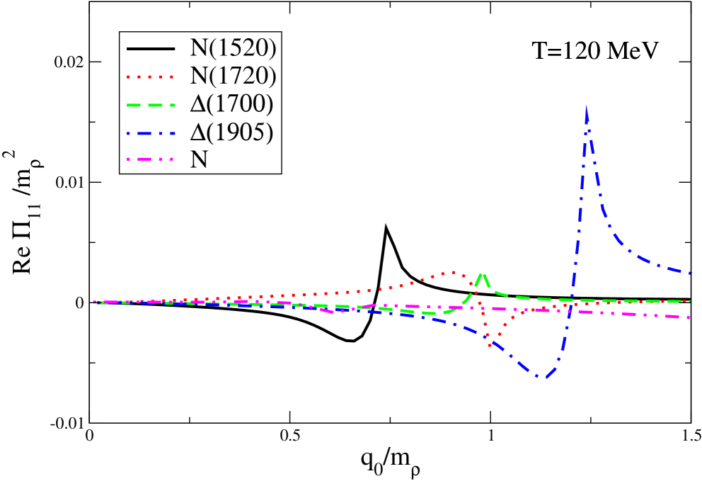
Figure 6: Contribution to the $\rho$ self-energy from scattering with nucleons and various other nucleon resonances. The main contribution for $q_{0}\sim m_{\rho}$ stems from the formation of $s$-channel, positive parity spin 3/2 N(1720) and spin 5/2 $\Delta$(1905) resonances.

The result is summarized in Fig. 6 where we show the temperature dependent real part of the self-energies scaled to the square of the $\rho$ mass in vacuum, for each of the resonances listed in Table I as a function of $q_{0}/m_{\rho}$, where $q_{0}$ is the energy of the $\rho$ meson at rest, for a temperature $T=120$ MeV. Notice that the two Feynman diagrams of Fig. 5 represent the contribution to the scattering process from nucleons and anti-nucleons, as corresponds to the scenario where resonance production happens from the –almost baryon free– central region of the reaction. The main contributions in magnitude for $q_{0}\sim m_{\rho}$ come from the resonances with even parity N(1720) and $\Delta$(1905). We also show the contribution from scattering with nucleons, taking $m_{N}$ to its vacuum value. Notice that for the kinematical range considered, the contribution from nucleons is completely negligible.

IV Interactions of $\rho$ with pions and other mesons

We now look at the contribution to the $\rho$ self-energy stemming from scattering with pions and other mesons. Table II shows the quantum numbers of those mesons with sizable branching ratios involving the pion and $\rho$ and whose rest mass is near the sum of the rest masses of the pion/kaon and $\rho$, as well as the coupling constants used in the calculation. For the interaction of $\rho$ and the pion, $\pi$, we take the Lagrangian

$${\mathcal{L}}=g_{\mbox{\tiny{$\rho\pi\pi$}}}\pi(\stackrel{{\scriptstyle\leftrightarrow}}{{\partial}}\ \!\!\!^{\mu}-ig_{\mbox{\tiny{$\rho\pi\pi$}}}\rho^{\mu})\pi\rho_{\mu}$$ (38)

obtained by gauging the pion-pion interaction Lagrangian Gale ; Ayala . The value of the dimensionless coupling constant, as determined by the $\rho$ width in vacuum, is taken as $g_{\mbox{\tiny{$\rho\pi\pi$}}}=6.06$ Gale .

The interaction Lagrangians involving the other relevant mesons are taken as Rapp

$${\mathcal{L}}=\left\{\begin{array}[]{l}g_{\mbox{\tiny{$\rho PA$}}}{\mathcal{F}}_{\rho PA}\ A^{\mu}\partial^{\nu}PF_{\mu\nu}\\ g_{\mbox{\tiny{$\rho\pi V$}}}{\mathcal{F}}_{\rho\pi V}\ \epsilon_{\mu\nu\sigma\tau}\partial^{\mu}\pi V^{\nu}\partial^{\sigma}\rho^{\tau}\\ (g_{\mbox{\tiny{$\rho\pi P^{\prime}$}}}/m_{\rho}){\mathcal{F}}_{\rho\pi P^{\prime}}\ \partial^{\mu}\pi\partial^{\nu}P^{\prime}F_{\mu\nu}\\ \end{array}\right.$$ (42)

where $V^{\mu}$ and $A^{\mu}$ represent the vector and axial-vector fields and $P$, $P^{\prime}$ the pseudo-scalar fields. ${\mathcal{F}}_{\rho PR}$ are dipole form factors [see Eq. (12)]. The coupling constants $g_{\mbox{\tiny{$\rho PR$}}}$ in Eqs. (42) are taken from Ref. Rapp . The interaction Lagrangians in Eqs. (38) and (42) are current and parity conserving as well as compatible with chiral symmetry.

$R$	$J^{P}$	$\rho h$ decay	$\Gamma^{\mbox{\tiny{vac}}}_{\rho h}$	$\Gamma^{\mbox{\tiny{vac}}}_{\mbox{\tiny{tot}}}$	$g_{\rho hR}$	$IF$
			(MeV)	(MeV)	${\mbox{(GeV)}}^{-1}$
$\omega$(782)	$1^{-}$	$\rho\pi$	$\sim 5$	$8.43$	25.8	1
$h_{1}$(1170)	$1^{+}$	$\rho\pi$	seen	$\sim 360$	11.37	1
$a_{1}$(1260)	$1^{+}$	$\rho\pi$	dominant	$\sim 400$	13.27	2
$K_{1}$(1270)	$1^{+}$	$\rho K$	$\sim 60$	$\sim 90$	9.42	2
$\pi^{\prime}$(1300)	$0^{-}$	$\rho\pi$	seen	$\sim 400$	7.44	2

Table 2: List of meson resonances included in the calculation. The last column corresponds to the isospin factor accounting for the number of isospin channels that take part in the dispersion. The coupling constants are taken from the analysis in Ref. Rapp .

The expressions for the one-loop $\rho$ self-energy corresponding to the interaction Lagrangians in Eqs. (42), can be written in Minkowski space, as

$$\Pi^{(J^{P})}_{\mu\nu} \!\!\!=\!\!\! IF\int\frac{d^{4}p}{(2\pi)^{4}}\frac{M^{(J^{P})}_{\mu\nu}}{[P^{2}-m_{\mbox{\tiny{P}}}^{2}][(P-Q)^{2}-m_{R}^{2}]}$$ (43)

where $m_{\mbox{\tiny{P}}}$ is the mass of the pseudoscalar ($\pi$ or $K$) and $m_{R}$ is the mass of the vector, axial-vector or $\pi^{\prime}(1300)$ and $IF$ is the isospin factor. The numerators in Eq. (43) are given by

$$M^{(1^{\pm})}_{\mu\nu} = \Gamma_{\mu\alpha}^{(1^{\pm})}\left(g^{\alpha\beta}-\frac{K^{\alpha}K^{\beta}}{m_{R}^{2}}\right)\Gamma_{\beta\nu}^{(1^{\pm})}$$

$$M^{(0^{+})}_{\mu\nu} = \Gamma_{\mu}^{(0^{+})}\Gamma_{\nu}^{(0^{+})}\,,$$ (44)

where $K=Q-P$ and the vertices, as obtained from the interaction Lagrangians in Eqs. (42), are given by

$$\Gamma_{\alpha\beta}^{(1^{+})} = g_{\mbox{\tiny{$\rho PA$}}}{\mathcal{F}}_{\rho PA}\ [g_{\alpha\beta}(P\cdot Q)-P_{\alpha}Q_{\beta}]$$

$$\Gamma_{\alpha\beta}^{(1^{-})} = g_{\mbox{\tiny{$\rho\pi V$}}}{\mathcal{F}}_{\rho\pi V}\ [\epsilon_{\gamma\alpha\delta\beta}(Q-P)^{\gamma}Q^{\delta}]$$

$$\Gamma_{\alpha}^{(0^{+})} = (g_{\mbox{\tiny{$\rho\pi P^{\prime}$}}}/m_{\rho}){\mathcal{F}}_{\rho\pi P^{\prime}}$$ (45)

$$[Q\cdot(Q-P)P_{\alpha}-(P\cdot Q)(Q-P)_{\alpha}]$$

It is easy to check that the explicit expressions for $M^{(1^{\pm})}_{\mu\nu}$ and $M^{(0^{+})}_{\mu\nu}$ are given by

$$M^{(1^{+})}_{\mu\nu} = g_{\mbox{\tiny{$\rho PA$}}}^{2}{\mathcal{F}}_{\rho PA}^{2}$$

$$\left\{[P^{2}Q^{2}-(P\cdot Q)^{2}]\ Q_{\mu\nu}+Q^{2}\ K_{\mu\nu}\right\}$$

$$M^{(1^{-})}_{\mu\nu} = g_{\mbox{\tiny{$\rho\pi V$}}}^{2}{\mathcal{F}}_{\rho\pi V}^{2}$$

$$\left\{-(P\cdot Q)^{2}\ Q_{\mu\nu}+Q^{2}\left(1-\frac{Q^{2}}{m_{R}^{2}}\right)K_{\mu\nu}\right\}$$

$$M^{(0^{+})}_{\mu\nu} = (g_{\mbox{\tiny{$\rho\pi P^{\prime}$}}}/m_{\rho})^{2}{\mathcal{F}}_{\rho\pi P^{\prime}}^{2}Q^{4}\ K_{\mu\nu}\,,$$ (46)

where the presence of the tensors $Q_{\mu\nu}$ and $K_{\mu\nu}$, defined in Eqs. (21), makes it evident that Eqs. (46) are explicitly transverse.

For the computation of the contributions to the thermal modifications of the $\rho$ mass, we work in the imaginary-time formalism of thermal field theory writing Eq. (43) in Euclidian space

$$\!\!\!\!\!\!\Pi^{(J^{P})}_{\mu\nu} \!\!\!=\!\!\! T\sum_{n}\int\frac{d^{3}p}{(2\pi)^{3}}\frac{M^{(J^{P})}_{\mu\nu}}{[P^{2}-m_{\mbox{\tiny{P}}}^{2}][(Q-P)^{2}-m_{R}^{2}]}$$ (47)

where $p_{0}=i\omega_{n}$ and $q_{0}=i\omega$, with $\omega_{n}=2n\pi T$ and $\omega=2m\pi T$ being boson Matsubara frequencies, and $n$ and $m$ integers. Once again, for definitiveness, we take the $\hat{z}$ axis as the direction of motion of the $\rho$ meson and thus the square of its thermal mass can be computed from the thermal part of the component $\Pi^{(J^{P})}_{11}$ in Eq. (43) in the limit of vanishing three-momentum.

From Eqs. (46) and (47), we must carry out sums over Matsubara frequencies of the form

$$S_{l}=T\sum_{n}(i\omega_{n})^{l}\Delta(i\omega_{n},E_{N})\Delta(i(\omega-\omega_{n}),E_{R})\,,$$ (48)

where $l=0,1,2$ and

$$\Delta(i\omega_{n},E)=\frac{1}{\omega_{n}^{2}+E^{2}}\,.$$ (49)

The sums for the cases $l=0,1$ are well known LeBellac and are given by

$$S_{0} = \sum_{s_{1},s_{2}=\pm}-\frac{s_{1}s_{2}}{4E_{P}E_{R}}\frac{1+n(s_{1}E_{P})+n(s_{2}E_{R})}{i\omega-s_{1}E_{P}-s_{2}E_{R}}$$

$$S_{1} = \sum_{s_{1},s_{2}=\pm}-\frac{s_{2}}{4E_{R}}\frac{1+n(s_{1}E_{P})+n(s_{2}E_{R})}{i\omega-s_{1}E_{P}-s_{2}E_{R}}\,,$$ (50)

where $n(E)$ is the Bose-Einstein distribution given in Eq. (3).

It is easy to check that the expression for $S_{2}$ is given by

$$S_{2}\rightarrow E_{P}^{2}S_{0}-\frac{n(E_{R})}{E_{R}}\,,$$ (51)

where the arrow indicates that we just consider the temperature dependent terms.

Using Eqs. (50) and (51) into Eq. (47) we can now make the analytical continuation $i\omega\rightarrow q_{0}+i\epsilon$ to compute the real part of the self-energies $\Pi_{11}^{(J^{P})}$, in a similar fashion as the one explained in detail in Sec. II. The result is summarized in Fig. 7 where we show the temperature dependent real part of $\Pi_{11}$ scaled to the square of the $\rho$ mass in vacuum arising from pion exchange as well as each of the mesons listed in Table II as a function of $q_{0}/m_{\rho}$, for a temperature $T=120$ MeV. We notice that in the interval considered, the main contribution comes from scattering of $\rho$ off pions. However, for $q_{0}\sim m_{\rho}$ a sizable contribution in magnitude comes from $\pi$–$\rho$ scattering through the formation of an $s$-channel axial-vector resonance $a_{1}$, which has the opposite sign and about the same strength as the contribution from pion exchange, in agreement with the findings in Ref. Rapp . Also, for $q_{0}\sim m_{\rho}$, the rest of the contributions offset among themselves.

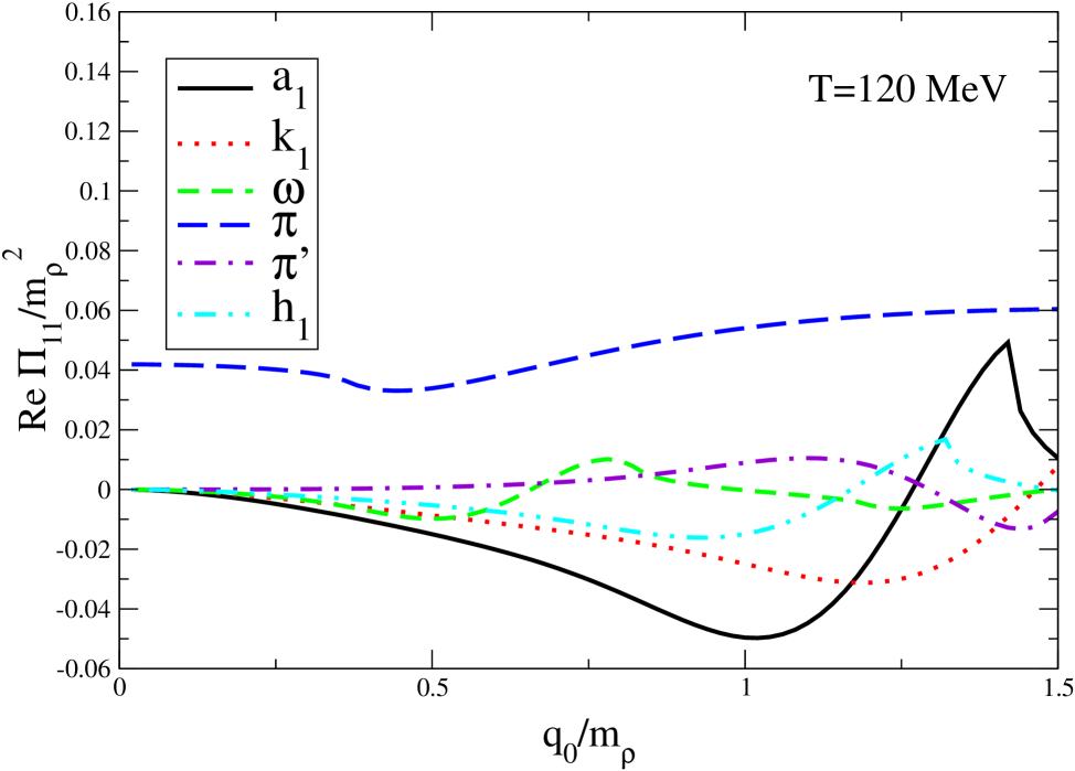
Figure 7: Contribution to the $\rho$ self-energy from scattering with pions and various other mesons. The main contribution for $q_{0}\sim m_{\rho}$ stems from the formation of an $s$-channel axial-vector resonance $a_{1}$.

V Intrinsic thermal mass of the $\rho^{0}$

We now put together the contributions from all of the particles considered in Secs. III and IV. This is summarized in Fig. 8 where we show the total shift in the intrinsic $\rho$ mass as a function of temperature. Notice that the shift is negative and increases in magnitude as the temperature increases. For instance, taking $m_{\rho}=770$ MeV, we get $M_{\rho}=764$–$730$ MeV when the temperature varies between $T=120$–$180$ MeV, which is a reasonable range for the temperature of the hadronic phase of a relativistic heavy-ion collision between chemical and kinetic freeze-out.

VI Summary and conclusions

In this work we have computed the intrinsic changes in the $\rho$ mass due to scattering with the relevant mesons and baryons in the context of ultra-relativistic heavy-ion collisions, at finite temperature. We have shown that a consistent field theoretical calculation of the real part of the one-loop $\rho$ self-energy yields the contributions form $t$- and $s$-channel scattering and that in general, both have to be accounted for. In addition to the already well know contributions arising from $\rho$ scattering with pions through the exchange of $a_{1}$ and pions themselves, we have found that the contributions from scattering with nucleons through the formation of even parity, spin 3/2 [N(1720)] and 5/2 [$\Delta$(1905)] nucleon resonances are significant.

The reason for the difference in the behavior between the real parts of the contributions of N(1720) and $\Delta(1905)$ to the $\rho$ self-energy as a function of $q_{0}$ –the former starting out repulsive and the latter attractive– is that the structure of their propagators and couplings with nucleons is different, given that these are resonances with different spin. The leading term for each case when $q_{0}\rightarrow 0$ is of the form $c*q_{0}$ where $c$ is a numerical coefficient to which several terms from the product of the propagator and vertices contribute. It turns out that this coefficient is positive in the case of N(1720) and negative in the case of $\Delta(1905)$. We emphasize that this conclusion is born out of the explicit calculation. We should however point out that an important cross check of the result, namely, the transversality of the self-energy, has been carried out. This is by no means a trivial check of the consistency of the calculation since had one or more of the terms that make up the above mentioned $c$ coefficient been wrong, the transversality would have been spoiled.

The results underline the importance of scattering of $\rho$ mesons with baryons, in particular nucleons at finite temperature, for the decrease of the intrinsic mass of $\rho$, during the hadronic phase of the reaction.

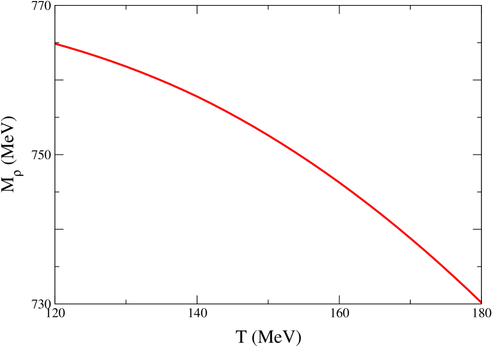
Figure 8: Intrinsic mass of $\rho^{0}$ as a function of temperature.

We have shown that it is possible to achieve a shift in the intrinsic $\rho^{0}$ mass of order $\sim-40$ MeV, when including the contributions of all the relevant mesons and baryons that take part in the scattering, for temperatures within the commonly accepted values for the hadronic phase of the collision, between chemical and kinetic freeze-out. These findings refer to the intrinsic changes in the $\rho$ mass. The overall change in the value of the peak of the invariant $\pi^{+}\ \pi^{-}$ distribution should contain also the effects of phase-space distortions due to thermal motion of the decay products as well as the effect due to the change in the intrinsic $\rho$ width Kolb ; Rapp2 . This is work in progress and will be reported elsewhere.

References

- (1) G. Roche et al., (DLS Collaboration) Phys. Lett. B226, 228 (1989); S. Beedoe et al., (DLS Collaboration) Phys. Rev. C47, 2840 (1993); G. Agakichiev et al., (CERES Collaboration), Phys. Rev. Lett. 75, 1272 (1995); D. Adamová et al., (CERES/NA45 Collaboration), Phys. Rev. Lett. 91, 042301 (2003).
- (2) For a comprehensive review of the theoretical and experimental status on the subject see R. Rapp and J. Wambach, Adv. Nucl. Phys. 25, 1 (2000).
- (3) J. Adams et al., (STAR Collaboration), Phys. Rev. Lett. 92, 092301 (2004).
- (4) R. Rapp and C. Gale, Phys. Rev. C 60, 024903 (1999).
- (5) R. Rapp and J. Wambach, Eur. Phys. J. A6, 415 (1999); V.L. Eletsky, M. Belkacem, P.J. Ellis and J.I. Kapusta, Phys. Rev. C 64, 035202 (2001).
- (6) O. Teodorescu, A.K. Dutt-Mazumder and C. Gale, Phys. Rev. C 66, 015209 (2002).
- (7) B. Friman and H.J. Pirner, Nucl. Phys. A617, 496 (1997)
- (8) W. Peters, M. Post, H. Lenske, S. Leupold and U. Mosel, Nucl. Phys. A632, 109 (1998).
- (9) A. Ayala, J.G. Contreras and J. Magnin, Mass of the meson in ultrarelativistic heavy-ion collisions, hep-ph/0403220, to appear in Phys. Lett. B.
- (10) See for example M. LeBellac Thermal Field Theory, (Cambridge University Press, Great Britain, 1996).
- (11) K. Hagiwara et al., Phys. Rev. D 66, 010001 (2002) (2003 off year partial update for the 2004 edition can be found on the PDG web page http://pdg.lbl.gov/)
- (12) J.G. Rushbrooke, Phys. Rev. 143, 1345 (1966).
- (13) D.M. Brudnoy, Phys. Rev. Lett. 14, 273 (1965).
- (14) M. Napsuciale and J.L. Lucio M., Nucl. Phys. B494, 260 (1997).
- (15) R. Machleidt, Adv. Nucl. Phys. 19, 198 (1989).
- (16) C. Gale and J. Kapusta, Nucl. Phys. B357, 65 (1991).
- (17) A. Ayala and J. Magnin, Phys. Rev. C 68, 014902 (2003).
- (18) P.F. Kolb and M. Prakash, Phys. Rev. C 67, 044902 (2003).
- (19) R. Rapp, Nucl. Phys. A725, 254 (2003).