Are black holes over-produced during preheating?

Abstract

We provide a simple but robust argument that primordial black hole (PBH) production generically does not exceed astrophysical bounds during the resonant preheating phase after inflation. This conclusion is supported by fully nonlinear lattice simulations of various models in two and three dimensions which include rescattering but neglect metric perturbations. We examine the degree to which preheating amplifies density perturbations at the Hubble scale and show that at the end of the parametric resonance, power spectra are universal, with no memory of the power spectrum at the end of inflation. In addition we show how the probability distribution of density perturbations changes from exponential on very small scales to Gaussian when smoothed over the Hubble scale – the crucial length for studies of primordial black hole formation – hence justifying the standard assumption of Gaussianity.

I Introduction

Primordial black holes (PBHs) span a wide range of mass scales and are typically much smaller than the solar mass ($\sim 10^{33}{\rm g}$) and may be formed in the early universe carr . PBHs may form from the gravitational collapse of large density fluctuations at horizon (i.e. Hubble scale $k=aH$) crossing in the radiation dominated universe. A PBH formed at the Planck time $\sim 10^{-43}{\rm sec}$ will have a mass $\sim 10^{19}{\rm GeV}$, while masses around $\sim 10^{15}{\rm g}$ are formed at $\sim 10^{-23}{\rm sec}$ ( see for example carr2 ).

The evaporation time for a PBH mass $\sim 10^{15}{\rm g}$ is nearly the present age of the universe, so PBH with smaller masses than this would have evaporated in the past, unloading a potentially vast amount of entropy. The success of the standard cosmology and the observation of the cosmic rays severely constrains the abundance of PBHs for various masses and provides useful constraints on inflationary and early universe physics.

For example, Big Bang Nucleosynthesis limits the PBH abundance in the mass range $10^{6}\sim 10^{13}{\rm g}$, by limiting the entropy from Hawking radiation or requiring that it does not modify the cosmological composition of the light elements starobinskii . PBH of mass $10^{15}{\rm g}$ evaporating now will emit particles such as $\gamma$-rays which are constrained by observations of the extragalactic $\gamma$-ray background which imply ${\Omega}_{PBH}<10^{-8}$ page . For $>10^{15}{\rm g}$, the limit on the PBH abundance is obtained from requiring that ${\Omega}_{PBH}$ does not exceed unity.

These observational constraints on PBHs provide a powerful probe of the primordial fluctuations. The upper bound on the abundance of PBHs directly leads to that on the density fluctuation at horizon crossing when PBH are formed. Therefore the scales of fluctuations relevant to PBH formation are much smaller than those associated with the Cosmic Microwave Background and the large-scale structure. This makes studying PBHs important. In the past, for example, constraints on the density perturbation spectrum were obtained by studying PBH formation bringmann . While the requirement that PBHs are not over-produced yields useful information about the early universe, PBH can be an interesting dark matter candidate in smaller abundances ivanov .

In this paper we will show that typically PBH are not over-produced during the violent non-equilibrium phase of preheating that follows the end of many inflationary models. This follows from three key observations: (1) the peak of the density perturbation spectrum typically lies at scales smaller than the Hubble scale. (2) The peak corresponds to density contrasts of order unity. (3) The slope of the spectrum around the horizon size is three (in $3d$). Putting these together we typically find that at the horizon scale relevant for PBH formation, the density contrast is around an order of magnitude too small to over-produce PBH. Nevertheless, the density perturbation on the horizon scale is significantly enhanced by preheating (by several orders of magnitude) compared with the no-resonance case and hence preheating is important in understanding the potential astrophysical and cosmological implications of PBH.

In studying the production of PBHs, one usually assumes that the probability distribution of density fluctuations at horizon crossing is Gaussian. This assumption is critical because the density perturbations which collapse to black holes are very rare: several $\sigma$ fluctuations (otherwise PBH will be over-produced in all cases) and therefore production of PBHs is sensitive to the tail of the distribution. Indeed Bullock and Primack bullock found that in some inflation models large perturbations are suppressed relative to a Gaussian distribution, resulting in a significant change in a number of PBH. We study the validity of the Gaussian assumption in a later section.

Among various possible scenarios that might over-produce PBHs, we focus on preheating after inflation. Preheating is a process in which energy transfer occurs rapidly from inflaton field to another field due to the non-perturbative effects during the oscillating phase of the inflaton traschen . This process significantly differs from the usual reheating scenario, where inflaton decays perturbatively to another particles, in a sense that in preheating most energies of inflaton field converts to created particles only during the several oscillations of inflaton and even the massive particle which is much heavier than the inflaton can be created. It has been understood that parametric resonance occurs generically at the first stage of reheating kofman1 . The parametric resonance does not last long because the rapid increase of created particles eventually affect the motion of background field and the created particles scatter off each other, removing the particles from the resonance band. By these effects, the resonance becomes inefficient and the decaying process of inflaton is described by usual single-body decay theory which finally leads to the thermal equilibrium state felder00 .

There are many works on preheating. The first stage of preheating, where the backreaction is negligible and the linear approximation is valid, was studied in detail in kofman2 ; pgreene ; shtanov . Parametric resonance including metric perturbations in order to see the behavior on super horizon scales were studied in taruya ; kodama ; bassett1 ; bassett2 ; finelli1 ; jedamzik ; liddle . As in the case without metric perturbations, there is a crucial difference between the single and multiple field cases. The analysis of fully non-linear preheating including gravity is very difficult. Before now, different approximations such as mean-field approximation bassett2 ; jedamzik ; zibin ; bassett3 ; bassett4 ; tsujikawa ; boyanovsky , lattice simulation lattice without metric perturbation and one dimensional fully non-linear calculations finelli2 ; parry ; easther have been done for studying the various effects caused by preheating on the present universe.

Green and Malik agreen argued that PBHs will be overproduced due to the amplification of fluctuations during preheating for many parameter regions in a two-field massive inflation model based on the results of liddle2 , which takes into account of the second order fluctuation of $\chi$ field. Put simply, their results suggested that the backreaction timescale was smaller than the timescale for the over-production of PBH.

Bassett and Tsujikawa bassett3 studied PBH production in the two-field massless inflation model including the effect of backreaction via the Hartree-Fock approximation and found that PBH overproduction might occur, if the probability distribution of fluctuation at horizon crossing was assumed to be chi-squared (which lowers the threshold mass variance, $\sigma$). However, they found that PBH were not over-produced if the distribution was assumed to be Gaussian and the density field was smoothed on the scale of the horizon. Nevertheless, that analysis was limited since it neglected the mode-mode coupling effects of rescattering and hence there was an open question both as to the underlying probability distribution of the density fluctuations and the contribution of rescattering to horizon-scale fluctuations.

We address both of these issues in this paper. We study PBH production due to preheating via two and three-dimensional lattice simulations which automatically include the effects of backreaction and rescatterings. We modified the C++ code LATTICEEASY written by Felder and Trachev latticeeasy . In lattice simulations, the evolution equations for the scalar fields (and also the scale factor) are solved in real (as opposed to Fourier) space ($N=2048^{2}$ for 2 dimensional simulation and $N=128^{3}$ for 3 dimensional simulation). Metric perturbations were not included, so we cannot apply this method to the dynamics on super horizon scales. We followed the evolution of both the scalar fields and the total density perturbation. We found that PBH are not overproduced and, interestingly, that the power spectrum at the end of preheating has a universal feature, that is, it is determined by the preheating dynamics and does not depend on the initial conditions. We also studied the probability distribution of the density perturbation at horizon crossing and found that it remained Gaussian which seems to be valid even in the tail of distribution.

A brief summary of our paper is as follows. Section II gives a brief review of calculating the PBH abundance formed from the large density perturbation. Section III describes the model of preheating in this simulation. In section IV, we consider the initial conditions of scalar fields. Section V shows the numerical results of lattice simulation. We will interpret the non-linear behavior of fluctuations and study the production of PBHs. Section VI discusses the probability distribution of fluctuations at horizon crossing we assume Gaussian in usual and Section VII is a conclusion.

II PBH formation by parametric resonance

II.1 Abundance of PBHs

In this subsection, we briefly review the standard method to estimate the abundance of PBHs carr3 . In the radiation dominated universe PBHs will be produced if ${\delta}_{H}$, the amplitude of density perturbations $\delta$ smoothed over the horizon size in the comoving gauge, exceeds a certain threshold ${\delta}_{c}$ agreen2 ; harrison . From linear analysis the critical value of ${\delta}_{c}$ is roughly estimated to be $1/3$, but it is not independent of the initial density profile. Numerical study niemeyer suggest $\delta_{c}\sim 0.7$ for various initial density profiles(see also  shibata ).

Under the assumption that the probability distribution of density fluctuation at horizon crossing is Gaussian, the mass fraction of PBHs at the formation time, $\beta$, is estimated as

$$\beta={\int}_{{\delta}_{c}}^{\infty}d{\delta}_{H}\ P({\delta}_{H})\sim\frac{\sigma}{\sqrt{2\pi}{\delta}_{c}}\exp\left(-\frac{{\delta}^{2}_{c}}{2{\sigma}^{2}}\right),$$ (1)

where $\sigma^{2}$ is the variance of $\delta_{H}$. Since the mass fraction of PBHs increases in proportion to the scale factor in the radiation dominated universe, $\beta$ must be very small in order to satisfy the astrophysical constraints.

Roughly speaking, $\beta$ is observationally constrained to be smaller than about $10^{-20}$ for most of the range of PBH mass except for a small window at $M\approx 10^{15}$g, which corresponds to PBHs evaporating now. If we adopt $10^{-20}$ as the upper bound on $\beta$, the upper bound on $\sigma$ becomes $\sim 0.03$ and $\sim 0.08$ for ${\delta}_{c}=0.3$ and $0.7$, respectively, assuming a Gaussian distribution for $\delta$. Though there is uncertainty in ${\delta}_{c}$ it does not affect our conclusions in the range of values $0.3-0.7$. Therefore we adopt the smaller value $0.03$ as the upper bound on $\sigma$ to be conservative.

To estimate the variance of density perturbations at the horizon scale, we simply use the power spectrum ${\cal P}_{\delta}(aH)$, where $a$ and $H$ are, respectively, the scale factor and the Hubble parameter, and ${\cal P}_{\delta}(k)$ is defined by

$$\langle{\delta}_{k}{\delta}_{-k^{\prime}}\rangle=\frac{2{\pi}^{2}}{k^{3}}{\cal P}_{\delta}(k)\delta(\vec{k}-\vec{k^{\prime}}).$$ (2)

II.2 Models of parametric resonance

In this paper, we consider two simple models of preheating.

II.2.1 Conformal Models

Conformal models are models composed of two scalar field with the potential given by pgreene ,

$$V(\phi,\chi)=\frac{\lambda}{4}{\phi}^{4}+\frac{g^{2}}{2}{\phi}^{2}{\chi}^{2}.$$ (3)

Here $\phi$ is the inflaton field. We start our simulation at the time when $\phi$ drops down to $0.34m_{pl}$ pgreene , where $m^{2}_{pl}=1/G$. In the oscillating phase of the inflaton the universe is effectively radiation dominated for the potential quartic in fields when averaged in time.

As standard, we introduce rescaled fields by

$${\tilde{\phi}}=a\phi/\phi_{0},\ \ \ {\tilde{\chi}}=a\chi/\phi_{0},$$ (4)

where the scale factor $a$ is normalized to unity at the end of inflation, (i.e., at the beginning of preheating),

We also introduce the rescaled conformal time $\tilde{\eta}$, related to proper time $t$ by

$$ad\tilde{\eta}=\sqrt{\lambda}\phi_{0}dt.$$ (5)

Then, the equations of motion for this model become

$${\tilde{\phi}}^{\prime\prime}-\lambda^{-1}\triangle{\tilde{\phi}}+{\tilde{\phi}}^{3}+{g^{2}\over\lambda}{\tilde{\phi}}{\tilde{\chi}}^{2}-\frac{a^{\prime\prime}}{a}{\tilde{\phi}}=0,$$ (6)

$${\tilde{\chi}}^{\prime\prime}-\lambda^{-1}\triangle{\tilde{\chi}}+{g^{2}\over\lambda}{\tilde{\phi}}^{2}{\tilde{\chi}}-\frac{a^{\prime\prime}}{a}{\tilde{\chi}}=0,$$ (7)

where ^′ denotes the differentiation with respect to $\tilde{\eta}$. In the radiation dominated universe ( $a\propto\tilde{\eta}$) the last terms in Eqs. (6) and (7) proportional to $a^{\prime\prime}$ vanish, and thus these equation reduce to the Minkowski ones. This is only exactly true if $\phi$ were conformally coupled to the curvature but since this is a weak effect we neglect it.

The unperturbed background solution for ${\tilde{\phi}}$ is given by Jacobi’s elliptic cosine function, $\mbox{cn}(\tilde{\eta})$ pgreene . Then, linearized equations obey the so-called Lamé equation finkel with resonance parameters $3$ and $g^{2}/\lambda$ for $\phi$ and $\chi$, respectively. Hence, the growth rate of the longest wavelength mode for $\chi$ is solely determined by $g^{2}/\lambda$, and there is a strong resonance at the longest wavelengths for $g^{2}/\lambda=2,8,18,\cdots$. Roughly speaking, the largest wave number in the efficient resonant band is

$$k_{max}=\left({g^{2}\over\lambda}\right)^{1/4}\sqrt{\lambda}\phi_{0},$$ (8)

An outstanding feature of conformal models is that the modes which are amplified by parametric resonance do not change by cosmic expansion. The Lamé equation for $\phi$ also has instability bands, but the growth rate is small compared with the typical one for $\chi$ and limited to roughly the Hubble scale quartic ; pgreene .

In our lattice simulations the evolution of the scale factor $a$ is determined self-consistently by solving Friedmann equation with the spatially averaged energy density. In the simulation, $\lambda$ is fixed to $9\times 10^{-14}$ appropriate to the COBE normalization. We studied both $g^{2}/\lambda=2$ and $50$. In both cases there is parametric resonance of $\chi$ for $k=0$ mode in the linear regime. In the former, the $\chi$ background is not strongly suppressed while in the latter case the $\chi$ field is heavy and is strongly suppressed during inflation jedamzik ; liddle ; bassett2 .

II.2.2 Massive Inflaton Models

We also considered massive inflaton models with the potential

$$V(\phi,\chi)=\frac{m^{2}}{2}{\phi}^{2}+\frac{g^{2}}{2}{\phi}^{2}{\chi}^{2}.$$ (9)

When the inflaton field oscillates around the potential minimum, the equation of state of the inflaton is dust on average. This means that amplitude of the background inflaton field decreases as $\propto a^{-3/2}$. Therefore it is convenient to introduce rescaled fields as

$${\tilde{\phi}}=a^{3/2}\phi/{\phi}_{0},\ \ {\tilde{\chi}}=a^{3/2}\chi/{\phi}_{0},$$ (10)

where ${\phi}_{0}=0.193m_{pl}$. Then, until the back reaction due to parametric resonance becomes efficient, the amplitude of the background ${\tilde{\phi}}$ stays almost constant. In terms of rescaled fields the equations of motion are

$${\ddot{\tilde{\phi}}}-a^{-2}\triangle{\tilde{\phi}}-\frac{3}{2}{\dot{H}}{\tilde{\phi}}-\frac{9}{4}H^{2}{\tilde{\phi}}+m^{2}{\tilde{\phi}}+g^{2}a^{-3}{\tilde{\phi}}{\tilde{\chi}}^{2}=0,$$

$${\ddot{\tilde{\chi}}}-a^{-2}\triangle{\tilde{\chi}}-\frac{3}{2}{\dot{H}}{\tilde{\chi}}-\frac{9}{4}H^{2}{\tilde{\chi}}+g^{2}a^{-3}{\tilde{\phi}}^{2}{\tilde{\chi}}=0.$$

(11)

where $\dot{}$ denotes the differentiation with respect to the proper time. From these equations, in contrast to the conformal case, we see that the expansion of the universe affects the motion of scalar fields: the wavelength of each comoving mode is redshifted and the effective coupling between $\tilde{\phi}$ and $\tilde{\chi}$ is decreased.

The linearized equations of Eqs. (11) was extensively studied in kofman2 . The equation for $\chi$ approximately reduces to the so-called Mathieu equation and the evolution of $\chi$ field shows broad resonance for

$$q:=\frac{g^{2}{\phi}_{0}^{2}}{4m^{2}}\gg 1.$$ (12)

Huge amplification of $\chi$ occurs at each time when amplitude of the inflaton field becomes zero due to violation of the adiabatic condition $\dot{\omega}/\omega^{2}<1$ for the $\chi$-field frequency, $\omega$.

When the expansion of the universe is taken into account the parametric resonance shows stochastic behavior because the phase of the $\chi$ field is randomized. Despite the stochastic nature, the amplitude of $\chi$ field grows exponentially on average. The maximum wave number in the resonance band is given bykofman2 ,

$$k_{max}\sim mq^{1/4}.$$ (13)

In our simulations we adopt $m=10^{-6}m_{pl}$ indicated by the COBE normalization, and $g=10^{-3}$ as a representative which realizes strong resonance. With this choice of parameters, we have $q=10^{4}$ at the beginning of preheating.

II.3 Initial Conditions

Since the modes that our simulation covers are mostly on subhorizon scales, the initial conditions for the field fluctuations after inflation can be determined by the formula for the adiabatic vacuum. For example, for the $\chi$-field we have

$$\langle{\chi}_{k}{\chi}_{-k^{\prime}}\rangle=\frac{1}{2{\omega}_{k}}\delta(k-k^{\prime}),$$ (14)

where ${\omega}_{k}=\sqrt{m^{2}_{\chi}+k^{2}}$ and

$$m_{\chi}:=g\phi_{0},$$ (15)

is the effective mass evaluated at the end of inflation. Recall that we have set $a=1$ at that time. Since we consider the cases with $m_{\chi}/k_{max}=(g^{2}/\lambda)^{1/4}$ greater than unity ( for $g^{2}/\lambda=50$), the power spectrum of $\chi$ field is given by

$${\cal P}_{\chi}(k)\approx\frac{k^{3}}{4\pi g\phi_{0}^{3}},$$ (16)

for wavelengths relevant for parametric resonance.

We also use Eq. (14) as the initial condition for fluctuations of $\tilde{\phi}$, replacing $m_{\chi}$ in ${\omega}_{k}$ with

$$m_{\phi}:=\sqrt{3\lambda}\phi_{0},$$ (17)

in the conformal models and $m$ in the massive inflation models.

In the conformal model with $g^{2}/\lambda=2$, $\chi$ stays almost always massless during inflation. In this case the initial spectrum on the superhorizon size becomes scale invariant bassett2 ; zibin . However the precise initial power spectrum ( i.e. after inflation) of scalar fields on subhorizon scales is rather involved. So here, for simplicity, we approximated ${\cal P}_{\chi}$ as

$${\cal P}_{\chi}=\frac{1}{4{\pi}^{2}}(k^{2}+H^{2}),\ \ \ (a=1),$$ (18)

which is blue on small scales and flat on large scales, capturing the key features of the spectrum. We will see that the precise form has no effect on the final results.

In our simulations, we compute classical dynamics taking the variance of these initial quantum fluctuations as if it were statistical variance, as standard latticeeasy . During the early stage the evolution is in linear regime and amplification of the $\chi$ occupation number in the quantum picture is correctly described by the amplification of the perturbation amplitude in classical dynamics son . When the nonlinearity becomes important, the occupation number of modes relevant for resonance is far beyond unity. Hence, a classical treatment is justified at late epoch, too. Moreover as we will see later, our final conclusion is quite insensitive to initial conditions.

III Numerical Results

III.1 Conformal Models

III.1.1 $g^{2}/\lambda=50$ case

Figure 1: Evolution of the power spectrum of scalar fields and the total density perturbation for $g^{2}/\lambda=50$. The horizontal axis is comoving wave number normalized by the (effective) inflaton mass at the end of inflation $m_{\phi}$. Time flows vertically. Lines labeled as a, b, c, d, e and f are for times ${\tilde{\eta}}=0,50,60,70,80,100$ respectively. Thus during our range of simulation, the inflaton field oscillates about $100/7.4\sim 14$ times. An arrow pointing upward represents rapid increase of the amplitude of fluctuations of the inflaton field due to the initial parametric resonance, and the arrow pointing rightward shows rescattering: high energy particles are generated by mode-mode coupling and scattering of low energy particles.

Fig. 1 shows the time evolution of the power spectra of the $\phi$ and $\chi$ fields and density perturbations until the backreaction shuts off the parametric resonance. Let us first focus on the power spectra of $\phi$ and $\chi$ fields. Both the power spectra are proportional to $k^{3}$ at the beginning. This is because the mass of each field is larger than the highest momentum resolved by simulation. In the early stage of evolution linear perturbation is a good approximation. The maximal characteristic (Floquet) exponent ${\mu}_{max}$ for $\phi$ is $\sim 0.036$, while that for $\chi$ is $\sim 0.2$. Hence, in this early stage perturbations of $\chi$-field grow exponentially, but those of $\phi$-field almost stay constant. After a few oscillations of the inflaton field, the perturbations of $\phi$ suddenly start to grow. This can be understood as follows. From Eq. (6) , the equation of motion for $\tilde{\varphi}:=\tilde{\phi}-\langle\tilde{\phi}\rangle$ is

$$\tilde{\varphi}^{\prime\prime}-\lambda^{-1}\triangle\tilde{\varphi}+3\langle\tilde{\phi}\rangle^{2}\tilde{\varphi}+3\langle\tilde{\phi}\rangle\tilde{\varphi}^{2}+\tilde{\varphi}^{3}+{g^{2}\over\lambda}(\langle\tilde{\phi}\rangle+\tilde{\varphi})\tilde{\chi}^{2}=0.$$ (19)

As $\chi$ grows exponentially by the parametric resonance, the last term in Eq. (19), $\frac{g^{2}}{\lambda}\langle\tilde{\phi}\rangle\tilde{\chi}^{2}$, exceeds the term $3{\langle\tilde{\phi}\rangle}^{2}\tilde{\varphi}$. At this stage, the linear approximation for $\tilde{\varphi}$ breaks and $\tilde{\varphi}$ begins to grow proportional to $\tilde{\chi}^{2}$, whose characteristic exponent is $\sim 0.4$ kofman2 . This happens when $\tilde{\chi}$ exceeds a critical value,

$$\tilde{\chi}_{c}\sim\left(\frac{g^{2}}{3\lambda}\right)^{-1/2}\tilde{\varphi}^{1/2}.$$ (20)

At the largest wave number in the resonance band of $\chi$-field, the initial amplitude of $\tilde{\varphi}$ is given by $\approx\sqrt{k_{max}^{3}/4\pi\sqrt{\lambda}}$ $\approx(g^{2}/\lambda)^{3/8}\sqrt{\lambda/4\pi}$. Hence $\tilde{\chi}_{c}$ is estimated as

$$\tilde{\chi}_{c}\approx\left({g^{2}\over\lambda}\right)^{-1/16}\lambda^{1/4}\sim 10^{-3}.$$ (21)

This rough estimate is consistent with the results of our lattice simulations.

Exponential amplification due to parametric resonance still continues until the effect of backreaction becomes significant. Parametric resonance ends when the second term in Eq. (3) becomes equal to the first term, that is when $\tilde{\chi}$ is amplified to

$$\tilde{\chi}_{b}=\left(\frac{g^{2}}{\lambda}\right)^{-1/4}.$$ (22)

The initial amplitude of $\tilde{\chi}$ at the shortest resonant mode given in $(\ref{kmax})$ is $\approx\sqrt{k_{max}^{3}/m_{\chi}}\approx{(g^{2}/\lambda)}^{1/8}\sqrt{\lambda}$. Approximating the evolution of ${\tilde{\chi}}$ as ${\tilde{\chi}}\propto e^{\mu\tilde{\eta}}$, the time at which parametric resonance ends, $\tilde{\eta}_{f}$, is estimated by

$$e^{\mu\tilde{\eta}_{f}}=\left(\frac{g^{2}}{\lambda}\right)^{-3/8}\lambda^{-1/2}.$$ (23)

Solving Eq. (23), we have ${\tilde{\eta}}_{f}\sim 70$. This estimate is consistent with the result $\tilde{\eta}_{f}\sim 80$ read from Fig. 1. Since ${\tilde{\eta}}_{f}$ depends on the initial amplitude of $\tilde{\chi}$ logarithmically, $\tilde{\eta}_{f}$ does not depend so much on the parameter $g^{2}/\lambda$ as long as models associated with strong resonance are concerned kofman2 .

By the time when the backreaction becomes important, the amplitude on smaller scales also increases due to the effect of rescattering.

In three dimensions, at the time when the simulation ends, the shortest wavelength modes have the largest amplitude in the simulation. However, this seems to be an artifact due to lack of resolution. In the corresponding two dimensional simulations shown in Fig.2, we can also see the rescattering effect. In this case perturbations do not pile up near the shortest wavelength but peak at a finite value of $k$. This is indeed consistent with the picture that $\chi$ particles with very large kinetic energy $k\rightarrow\infty$, are not produced.

Let us now focus on the power spectrum of density perturbations. The energy density $\rho$ is given by

$$a^{4}\lambda^{-1}\rho=\frac{1}{2}{({\tilde{\phi}}^{\prime}-{\tilde{\cal H}}{\tilde{\phi}})}^{2}+\frac{1}{2}(\tilde{\chi}^{\prime}-\tilde{\cal H}\tilde{\chi})^{2}+\frac{1}{2\lambda}(\vec{\nabla}\tilde{\phi})^{2}$$

$$+\frac{1}{2\lambda}(\vec{\nabla}\tilde{\chi})^{2}+\frac{1}{4}\tilde{\phi}^{4}+\frac{g^{2}}{2\lambda}\tilde{\phi}^{2}\tilde{\chi}^{2},$$ (24)

where ${\tilde{\cal H}}:=\partial_{\tilde{\eta}}\log a$. From this equation, the density perturbations to first order are

$$a^{4}\lambda^{-1}\delta\rho\approx(\langle\tilde{\phi}\rangle^{\prime}-\tilde{\cal H}\langle\tilde{\phi}\rangle)(\varphi^{\prime}-\tilde{\cal H}\varphi)+\langle\tilde{\phi}\rangle^{3}\varphi.$$ (25)

As we have already mentioned, amplitude of $\varphi$ is almost constant in the linear perturbation regime. Therefore in this regime amplitude of density perturbations does not grow. This behavior of $\delta\rho$ can be observed in Fig. 1. When the amplitude of $\tilde{\chi}$ reaches $\tilde{\chi}_{c}$, the terms second order in field perturbations start to contribute to $\delta\rho$. Then, density perturbations begin to grow rapidly. After the exponential increase of $\delta\rho$, the amplification of density perturbations stops when the growth of field perturbations terminates due to back reaction to the oscillation of $\langle\tilde{\phi}\rangle$.

From Fig. 1, we find that the slopes of power spectrum of resultant density perturbations on large scales are all equal to three.

As we shall see below, this result does not change even if we artificially amplify the initial fluctuations of fields on large scales, which leads to the rule of thumb that after preheating correlation of perturbations on large scales disappears rather independently of initial power spectrum.

We can give a simple interpretation to this result. What we assume is that the resultant density perturbations have a typical scale $r$, and correlations on larger length scales are strongly suppressed. In such a situation, the integral

$${1\over k^{D}}{\cal P}_{\delta}(k)\propto\int d^{D}x\,\langle\delta(0)\delta({\vec{x}})\rangle e^{i\vec{k}\vec{x}},$$ (26)

is dominated by a small region with $|\vec{x}|\lesssim r$, where $D$ is the number of spatial dimensions, which is 3 in our simulation. For long wavelength modes with $k\ll r^{-1}$, $e^{i\vec{k}\vec{x}}$ can be approximated by unity. Thus we have

$${\cal P}_{\delta}(k)\propto k^{D},$$ (27)

We also performed 2 dimensional lattice simulations, and found the power spectrum proportional to $k^{2}$ on large scales as predicted; see (Fig. 2).

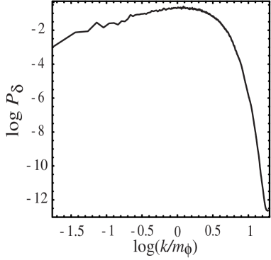
Figure 2: The power spectrum of density perturbation after preheating for two-dimensional space. We see that the slope of the power spectrum for small $k$ is two, as expected.

One may think that we have obtained this result because of the initial blue spectrum of $\chi$-field. Since the characteristic exponent of the parametric amplification is almost the same for all modes with $k/m_{\phi}<{(g^{2}/\lambda)}^{1/4}$, the parametric resonance will end due to the backreaction from the mode of the shortest resonance scale, at which the initial amplitude is the largest among the modes in resonance. At that time perturbations of $\chi$-filed still remain small on large scales (where by large scale we here mean around the horizon size and larger).

Here we show that the initial blue spectrum is not a necessary condition for suppression on large scales. For this purpose, we performed the same simulation but with the scale invariant initial spectrum (${\cal P}_{\chi}$=constant, where the power spectrum is initially amplified on large scales). Fig. 3 shows ${\cal P}_{\delta}$ after preheating in this case.

From this figure, we see that at the end of preheating perturbations on horizon scales are suppressed with slope 3, which is the same as in the case with the initial blue spectrum. This result indicates that in general parametric resonance causes loss of correlation between density fluctuations beyond a typical length

scale and energy is efficiently cascaded to shorter wavelengths by rescattering.

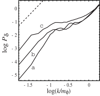
Figure 3: Power spectrum of the total density perturbation after preheating for three cases in three dimensions. Lines labeled as a, b and c correspond to $g^{2}/\lambda=50$, $g^{2}/\lambda=50$ with scale-invariant power spectrum and $g^{2}/\lambda=2$ respectively. We see that the slope of the power spectrum for small $k$ is universal with a value of three. The dashed line has $k^{3}$ power and crosses the threshold at the horizon scale. All three lines are lie significantly under the dashed line, showing that PBHs are not overproduced in these cases. The peak of the spectrum and subsquent decay are not resolved by our three dimensional simulations but are resolved in two dimensions.

In order to estimate the production rate of PBHs, we have to compute $\delta\rho/\rho$ smoothed over the horizon size. The horizon size when parametric resonance ends corresponds to $k=aH\approx 5\times 10^{-3}m_{\phi}$, which is not covered in our three-dimensional simulations.

However, since there is no typical length scale before the horizon scale, it will be natural to expect that one can extrapolate the power spectrum to horizon size assuming the slope of the power spectrum of density perturbations is $D$. The result of 2 dimensional simulations (Fig. 2) also support this extrapolation. With the aid of this extrapolation, the amplitude of density contrast at the horizon size ${\delta}_{H}$ can be estimated from Fig. 1 as

$${\delta}_{H}\sim 3\times 10^{-4},$$ (28)

which is an order of magnitude smaller than the threshold for PBH overproduction (0.03). Therefore we conclude it is unlikely that PBHs are overproduced by the parametric resonance in the case with $g^{2}/\lambda=50$.

III.1.2 $g^{2}/\lambda=2$ case

We also performed lattice simulations for $g^{2}/\lambda=2$. In this case, the power spectrum of $\chi$ at the end of inflation is flat for $k<H_{0}$, where $H_{0}$ is the Hubble parameter at the end of inflation. Therefore, the modes whose wave length is much larger than the horizon size is not suppressed in this case, which is different from the case 1 $g^{2}/\lambda\gg 1$ bassett2 . Taking into account the fact that there is a strong resonance at small $k$ for $g^{2}/\lambda=2$ , there is a possibility of PBHs overproduction in this case bassett3 ; agreen .

${\cal P}_{\delta}$ for $g^{2}/\lambda=2$ is shown in Fig. 3. As before, the power spectrum of $\delta$ after parametric resonance is suppressed and its slope is three around the horizon scale, implying that large scale perturbations are uncorrelated. Therefore in the same way as discussed in the case with $g^{2}/\lambda=50$, production of PBHs caused by parametric resonance will not be efficient enough to exceed the astrophysical bounds.

III.2 Massive Inflaton Models

Fig. 4 shows the evolution of the power spectrum during preheating for a massive inflaton model. From this figure we find that the power spectrum after preheating is $\propto k^{3}$ on horizon scales as in the case of conformal models.

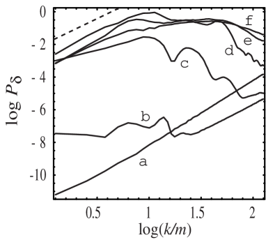
Figure 4: Evolution of the power spectrum of $\delta$ for the massive inflaton model. Lines labeld as a, b, c, d, e and f correspond to $mt=0,50,60,70,100,120$ respectively. The dashed line represents the threshold for PBH over-production which lies well above any of the curves.

Here we cannot directly use the criterion for the PBH production discussed in section II, because the universe is not radiation dominated but dust on average. Due to the difference of the equation of state, the condition that density perturbations collapse to form a black hole differs from the one in the radiation dominated universe. In carr3 , the critical density ${\delta}_{c}$ for the equation of state

$$P=\epsilon\rho,$$ (29)

depends on $\epsilon$. Here we assume that the instability of the density perturbation of scalar fields in massive inflaton models is similar to the fluid case with the same effective equation of state.

The energy density and pressure in massive inflaton models are

$$\rho=T+U,\qquad P=T-U,$$ (30)

with

$$T = \frac{1}{2}{\dot{\phi}}^{2}+\frac{1}{2}{\dot{\chi}}^{2},$$ (31)

$$U = \frac{1}{2}{(\frac{1}{a}\vec{\nabla}\phi)}^{2}+\frac{1}{2}{(\frac{1}{a}\vec{\nabla}\chi)}^{2}+\frac{m^{2}}{2}{\phi}^{2}+\frac{g^{2}}{2}{\phi}^{2}{\chi}^{2}.$$ (32)

Using the equations of motion for the scalar fields, we can show the relation,

$$\langle T\rangle=\langle U\rangle+\frac{g^{2}}{2}\langle{\phi}^{2}{\chi}^{2}\rangle,$$ (33)

where $\langle\cdots\rangle$ denotes a long time average with the weight $a^{3}\,dt$. Hence we can estimate $\epsilon$ by

$$\epsilon\approx\frac{g^{2}}{2}\langle{\phi}^{2}{\chi}^{2}\rangle/\langle\rho\rangle.$$ (34)

Fig. 5 shows the time evolution of this quantity during preheating.

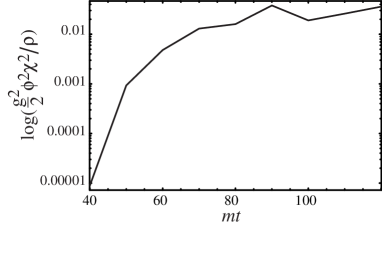
Figure 5: Time evolution of the ratio of the interaction energy $\frac{g^{2}}{2}{\phi}^{2}{\chi}^{2}$ to the total energy density $\rho$. Time is normalized in $1/m$. We see that $\epsilon$ after preheating is about $3\times 10^{-2}$, i.e. the total system behaves approximated as dust.

At the end of preheating $\epsilon$ becomes as large as $\sim 3\times 10^{-2}$. Therefore the ratio of pressure to energy density after preheating in massive inflaton model is ten times smaller than that of the radiation dominated universe. Hence, the upper limit on $\sigma$ in the case of massive inflaton model will be reduced to about $3\times 10^{-3}$. On the other hand, from Fig. 4, the value of the power spectrum of the density perturbation at horizon size ($k\approx 1\times 10^{-1}m$) can be estimated as

$${\delta}_{H}\sim 5\times 10^{-4},$$ (35)

where we have used the simulations to conclude that the power spectrum is proportional to $k^{3}$ for small $k$. This is smaller than the threshold $\sim 3\times 10^{-3}$ again by about one order of magnitude. Therefore we conclude that PBHs will not be overproduced in massive inflaton model, either, despite the fact that $\sigma$ is significantly enhanced by resonance on horizon scales.

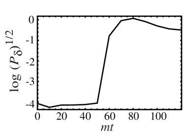
Figure 6: Time evolution of $\sqrt{{\cal P}_{\delta}}$ at $k=k_{max}=q^{1/4}m$. From this, we see that backreaction terminates the parametric amplification at around $mt=70$.

IV Gaussianity

In this section, we discuss the probablity distribution of the amplitude of density perturbations at the end of preheating. In the preceding sections we estimated the abundance of PBHs by assuming that the probability distribution of density perturbations at the horizon size is Gaussian. If the tale of distribution, which is relevant for PBH formation, had a non-Gaussian tail, the resultant astrophysical constraints would be significantly altered and hence it is a crucial assumption to test. Further, since rescattering ($\propto\delta\chi^{2}$) is crucial, one might expect chi-squared corrections to be important.

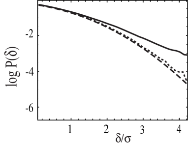
Figure 7: The probability distribution of density fluctuations smoothed over the scale $m_{\phi}$ (the Compton wavelength of the inflaton) in the conformal model. The dotted line is the spectrum at initial time and black line is the spectrum at the end of preheating. The dashed line is an appropriately scaled Gaussian distribution. At the end of preheating, the distribution of large fluctuations is significantly more amplified than the Gaussian prediction.

We first show the distribution of density fluctuation smoothed over the shortest resonant scale in a conformal model. The result is shown in Fig. 7. We can see that the distribution does not trace a Gaussian distribution at the end of preheating, while it does at the initial stage. In particular, the probability of large amplitude of perturbations is enhanced through preheating. Interestingly, the late time distribution looks like exponential.

This results can be understood as follows. At initial stage where the linear approximation is valid, density perturbation is just a superposition of Gaussian distributions. Hence, the probability distribution is Gaussian. As perturbations grow, the terms quadratic in field perturbations start to contribute to $\rho$. The probablity distribution in such situation will be mimiced by a product of two Gassian random variables $x$ and $y$. The probability distribution of $z=xy$ is given by

$$P(z) = \frac{1}{2\pi{\sigma}_{1}{\sigma}_{2}}\int\frac{dx}{x}e^{-\frac{x^{2}}{2}-\frac{z^{2}}{2{\sigma}^{2}_{1}{\sigma}^{2}_{2}}\frac{1}{x^{2}}}$$ (36)

$$\sim \frac{1}{2\sqrt{2\pi{\sigma}_{1}{\sigma}_{2}z}}e^{-\frac{z}{{\sigma}_{1}{\sigma}_{2}}},$$ (37)

where $\sigma_{x}^{2}$ and $\sigma_{y}^{2}$ are variances $x$ and $y$, respectively. Here in the last step we used the steepest decent method assuming $z$ is much larger than ${\sigma}_{1}{\sigma}_{2}$. In this manner one can reproduce a pure exponential distribution for large values of $z$.

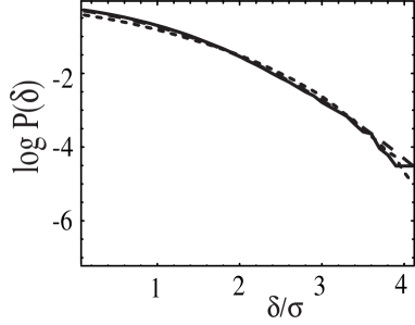
Figure 8: The probability distribution of density fluctuation smoothed over the scale $50\times m_{\phi}$ in the conformal model. The dotted line is the distribution at the initial time and the black one is at the end of preheating. Contrary to Fig. 7, the distribution is still Gaussian even at the end of preheating. Hence, on the horizon scale relevant to PBH production the Gaussian assumption is a good approximation.

Next we show the distribution of density perturbations averaged over a large scale. The result is shown in Fig. 8. In this case the distribution is almost Gaussian even at the end of preheating. This result can be interpreted as follows. As we discussed in section V, the density perturbations lose correlation on scales much larger than the shortest wavelength in the resonance band. Hence, the average over a large length scale $L$ behaves as a sum of a large number of independent random variables of $O\left((Lk_{max}/a)^{3}\right)$. Therefore its distribution is guaranteed to be close to Gaussian by the central limit theorem, which is consistent with numerical the results. Significant deviations from Gaussianity are not expected unless the amplitude is as about $(Lk_{max}/a)^{3}$ times larger than the standard deviation. Since the horizon size at the end of preheating is much larger than the shortest wavelength in the resonance band,

the required amplitude is extremely large, and hence the probability of finding it is completely negligible.

Hence, non-Gaussianity cannot affect the estimate of the PBH formation rate.

V The effect of metric perturbations

Finally we briefly discuss the role of gravitational interactions (metric perturbations) which might have effects on PBH formation. We have neglected them throughout this paper but there is a good reason why one expects that this is a good approximation. The time scale for gravitational collapse is at most free fall time. Unless density perturbations significantly exceed $O(1)$, this time scale is identical to the Hubble time scale. On the other hand parametric resonance undergoes with the time scale determined by the effective mass of the inflation, which is in general shorter than the Hubble time scale. Moreover, in the expanding universe gravitational instability does not grow exponentially, while parametric resonance drives exponential growth of perturbations. Hence, we expect gravitational interactions play a subdominant role at the stage of preheating, although later on a longer time scale gravitational collapse may proceed in cases where the effective pressure happens to be very small (such as in the massive model).

In the treatment neglecting the gravitational interaction, there arises another subtlety related to the gauge. We discussed the amplitude of density perturbations at the horizon size, but it is a gauge dependent quantity. Hence, strictly speaking, it is incorrect to quote the criterion for the PBH formation stated in terms of density perturbations in comoving gauge. Moreover, it is more suitable to use the amplitude of metric perturbations rather than density contrast niemeyer ; shibata .

In the present context, this is mainly because the power spectrum of density perturbation has a strong $k$-dependence, $\propto k^{3}$, which means that probability of PBH formation is very sensitive to the choice of the horizon size bassett3 . In contrast, since the metric perturbations well inside the horizon is characterized by the Newton potential, the power spectrum of metric perturbations will be proportional to $k^{-1}$. On the other hand, it was shown in tanaka that the curvature perturbation on the constant energy density hypersurfaces $\zeta$ (Bardeen parameter) behaves like $\propto k^{3}$ on super horizon scales after preheating by using the separate universe approach stewart ; taruya ; KH ; TS ; wands .

Therefore, say, the curvature perturbation $\zeta$ will have a peak near at the horizon size, and we will be able to obtain an unambiguous upper limit on the abundance of PBHs produced by preheating. From the above consideration, including metric perturbation in the evolution of scalar fields is an interesting issue which we leave for future work.

VI Summary and discussion

We have studied the formation of black holes during preheating after inflation. Preheating provides a challenging framework to illucidate various complex physical processes such as non-equilibrium, non-perturbative field theory in expanding backgrounds. In addition, since preheating is generic in some regions of parameter space for many inflationary models, the issue of whether primordial black holes (PBH) are overproduced is an important one.

To address this we have performed two and three dimensional lattice simulations of several different inflaton potentials (conformal and massive) and parameter regions. These simulations automatically incorporate all non-linear effects such as backreaction and rescattering of fields. We found no evidence for over-production of PBH, in contrast to earlier expectations. In addition we found that although highly non-Gaussian on very small scale, the spectrum of density perturbations is effectively Gaussain on the horizon (i.e. Hubble) scale.

Our results can be understood simply. For all cases, we found that when the amplitude of density perturbations at about the shortest wavelength in the resonant band becomes of order unity, the growth due to parametric resonance terminates due to backreaction. At the end of preheating the final density spectrum is universal, with a blue power spectrum, $\propto k^{D}$ (D = 2,3) on horizon scales, depending on whether the simulation was two ($D=2$) or three ($D=3$) dimensional. Since the peak of the spectrum is scales significantly shorter than the horizon scale, the amplitude of the density perturbation at the horizon scale extrapolated from the peak is typically about an order of magnitude below the threshold for PBH overproduction.

We gave an explanation of this universality in the slope of the final power spectrum on large scales as a result of loss of coherence due to parametric resonance.

These results argue for the view that generically PBHs will not be produced so much as to violate astrophysical constraints, even in the case of strong preheating. This result also applies to the cases with other models and parameters regions if our interpretation of the power spectrum on large scales is universally correct.

The result obtained in this paper is different from the claim by Green and Malik agreen , where they found that PBHs are likely to be overproduced. They estimated the time when backreaction becomes significant as well as the time when the amplitude of density perturbations exceeds the threshold separately based on linear approximation. Comparison of these two times was used to give a criteria for PBH formation. However, for example, in Ref. kofman2 the time when the backreaction becomes significant in the case with $m=10^{-6}m_{pl}$ and $g=10^{-3}$ is estimated to be $\sim 90$, which is slightly later than our numerical result (See Fig. 6). Since the growth of perturbation amplitude is exponential, a small error in the back reaction time can lead to wrong conclusions. In calculating the abundance of produced PBHs, only $10\sim 20$ percent error of backreaction time can lead to the opposite conclusion. By contrast, our conclusion is based on self-consistent simulations and rather robust qualitative observations. There is no delicate comparison of different time scales.

In this paper, we considered standard slow roll inflation. In such cases, preheating occurs at rather high energies. Therefore the mass of PBHs formed in the present context is too small to avoid evaporation before the Big Bang Nucleosynthesis. Hence, those PBHs are not subject to any observational constraint even if PBHs are produced abundantly, unless PBHs leave Planck mass relics barrow . (Hence we have assumed that PBH will leave Planck mass relic throughout this paper. ) Even if relics are formed, the constraint on the mass fraction of produced black holes is $\beta<10^{-20}$ carr5 , we can therefore conclude that production of PBHs by preheating does not give a serious constraint on such simple models of preheating as discussed in this paper.

However, our qualitative results will also apply for preheating at lower energies. Let us consider the possibility of making more massive black holes by preheating, say, in the case of massive inflaton models. Now we consider to vary the inflaton mass $m$ and the value of $\phi$-filed at the beginning of preheating $\phi_{0}$ within $\phi_{0}\lesssim m_{pl}$ (As an example of realizing small value of $\phi_{0}$, we can consider the hybrid inflation model linde .). The key quantity is the ratio of $k_{max}$ given in (13) to the Hubble parameter, which is estimated as

$$\frac{k_{max}}{H}\sim\frac{m_{pl}}{\phi}q^{1/4}.$$ (38)

This ratio is independent of $m$ and is the smallest for $\phi\approx m_{pl}$. Then the same estimate given in (35) applies as an upper bound for $\delta_{H}$. On the other hand, lowering $\beta$ down to $10^{-30}$ only change the upper bound on $\sigma$ from 0.031 to 0.026. Thus we can say that overproduction of more massive PBHs due to parametric resonance is also unlikely.

We have also confirmed Gaussianity of the probability distribution of density perturbations at the horizon scale, which is assumed in the estimate of the production rate of PBHs. The appearance of Gaussianity is in accordance with the interpretation of the spectrum on large scales. If perturbations become uncorrelated beyond the shortest resonant scale, perturbations at the horizon scale are given by average of many statistically independent random variables. Thus Gaussianity naturally follows from the central limit theorem.

- (1) B. J. Carr and S. W. Hawking, Mon. Not. R. Astron. Soc. , 399(1974).
- (2) B. J. Carr, astro-ph/0310838.
- (3) K. Kohri and J. Yokoyama, Phys. Rev. D , 023501(1999); P. D. Nasel’skii, Sov. Astron. Lett. , 4; T. Rothman and R. Matzuer, Astrophys. Space. Sci. , 229(1981); D. Lindley, Mon. Not. R. Astron. Soc. , 593(1980); S. Miyama and K. Sato, Prog. Theor. Phys. , 1012(1978); Ya. B. Zel’dovich and A. A. Starobinskii, Pis’ma Zh. Eksp. Teor. Fiz. , 616(1976).
- (4) D. N. Page and S. W. Hawking, Astrophys. J. , 1(1976); I. D. Novikov, A. G. Plonarev, A. A. Starobinsky and Ya. B. Zel’dovich, Astron. Astrophys. , 104(1979).
- (5) T. Bringmann, C. Kiefer and D. Polarski, astro-ph/0109404; B. J. Carr, J. E. Lidsey, Phys. Rev. D , 543(1993); H. I. Kim and C. H. Lee, Phys. Rev. D , 6001(1996); A. M. Green and A. R. Liddle, Phys. Rev. D , 6166(1997).
- (6) J. D. Barrow, E. J. Copeland and A. R. Liddle, Phys. Rev. D , 645(1992);
- (7) B. J. Carr, J. H. Gilbert and J. E. Lidsey, Phys. Rev. D , 4853(1994);
- (8) P. Ivanov, P. Naselsky and I. Novikov, Phys. Rev. D , 7173(1994); T. Nakamura, M. Sasaki, T. Tanaka and K. S. Thorne, Astrophys. J. , L139(1997); N. Afshordi, P. McDonald and D. N. Spergel, Astrophys. J. , L71(2003); T. Kanazawa, M. Kawasaki and T. Yanagida, Phys. Lett. , 174(2000); M. Kawasaki, N. Sugiyama and T. Yanagida, Phys. Rev. D , 6050(1998).
- (9) J. S. Bullock and J. R. Primack, Phys. Rev. D , 7423(1997); J. S. Bullock and J. R. Primack, astro-ph/9806301.
- (10) J. H. Traschen and R. H. Brandenberger, Phys. Rev. D , 2491(1990); H. Fugisaki, K. Kumekawa, M. Yamaguchi and M. Yoshimura, Phys. Rev. D , 6805(1996).
- (11) L. Kofman, A. Linde and A. A. Starobinsky, Phys. Rev. Lett. , 3195(1994);
- (12) G. Felder and L. Kofman, Phys. Rev. D , 103503(2000);
- (13) L. Kofman, A. Linde and A. A. Starobinsky, Phys. Rev. D , 3258(1997);
- (14) P. B. Greene, L. Kofman, A. Linde and A. A. Starobinsky, Phys. Rev. D , 6175(1997); D. I. Kaiser, Phys. Rev. D 57, 702 (1998)
- (15) D. Boyanovsky, M. D’Attanasio, H. J. de Vega, R. Holman and D. S. Lee, Phys. Rev. D 52, 6805 (1995)
- (16) Y. Shtanov, J. Trachen and R. H. Brandenberger, Phys. Rev. D , 5438(1995).
- (17) D. T. Son, arXiv:hep-ph/9601377.
- (18) A. Taruya and Y. Nambu, Phys. Lett. , 37(1998).
- (19) F. Finelli and R. H. Brandenberger, Phys. Rev. D , 083502(2000);
- (20) H. Kodama and T. Hamazaki, Prog. Theor. Phys. , 949(1996);
- (21) B. A. Bassett, D. I. Kaiser and R. Maartens, Phys.Lett. , 84(1999); B. A. Bassett, F. Tamburini, D. I. Kaiser and R. Maartens, Nucl. Phys. B. , 188(1999);
- (22) A. R. Liddle, D. H. Lyth, K. A. Malik and D. Wands, Phys. Rev. D , 103509(2000);
- (23) B. A. Bassett and F. Viniegra, Phys. Rev. D , 043507(2000).
- (24) K. Jedamkik and G. Sigl, Phys. Rev. D , 023519(1999);
- (25) J. P. Zibin, R. Brandenberger and D. Scott, hep-ph/0007219;
- (26) B. A. Bassett and S. Tsujikawa, Phys. Rev. D , 123503(2001).
- (27) B. A. Bassett and F. Tamburini, Phys. Rev. Lett. , 2630(1998).
- (28) S. Tsujikawa, K. Maeda and T. Torii, Phys. Rev. D , 063515(1999).
- (29) D. Boyanovsky et al. , Phys. Rev. D , 1939 (1997).
- (30) S. Yu. Khlebnikov and I. I. Tkachev, Phys. Rev. Lett. , 1607(1997); S. Yu. Khlebnikov and I. I. Tkachev, Phys. Rev. Lett. , 219(1996); S. Khlebnikov and I. Tkachev, Phys. Rev. D , 653(1997); S. A. Ramsey and B. L. Hu, Phys. Rev. D , 678(1997);
- (31) F. Finelli and S. Khlebnikov, Phys. Rev. D , 043505(2002);
- (32) M. Parry and R. Easther, Phys. Rev. D , 061301(1999); M. Parry and R. Easther, gr-qc/0105117;
- (33) R. Easther and M. Parry, Phys. Rev. D , 103503(2000).
- (34) A. M. Green and K. A. Malik, Phys. Rev. D , 021301(2001).
- (35) A. R. Liddle, D. H. Lyth, K. A. Malik and D. Wands, Phys. Rev. D , 103509(2000).
- (36) G. Felder and I. Tkachev, hep-ph/0011159, see also http://physics. stanford. edu/gfelder/latticeeasy.
- (37) B. J. Carr, Astrophys. J. , 1(1975)
- (38) A. M. Green, A. R. Liddle, K. A. Malik and M. Sasaki, astro-ph/0403181.
- (39) E. R. Harrison, Phys. Rev. D , 2726(1970).
- (40) J. C. Niemeyer and K. jedamzik, Phys. Rev. Lett. , 5481(1998); J. C. Niemeyer and K. jedamzik, Phys. Rev. D , 124013(1999).
- (41) M. Shibata and M. Sasaki, Phys. Rev. D , 084002(1999).
- (42) A. R. Liddle and D. H. Lyth, Phys. Rep. , 1(1993).
- (43) F. Finkel, A. González-López, A. L. Maroto and M. A. Rodríguez, Phys. Rev. D , 103515(2000).
- (44) T. Tanaka and B. Bassett, in proceedings of 12th workshop on General Relativity and Gravitation in Japan, astro-ph/0302544.
- (45) M. Sasaki and E. D. Stewart, Prog. Theor. Phys. 95, 71 (1996).
- (46) H. Kodama and T. Hamazaki, Phys. Rev. D 57, 7177 (1998).
- (47) M. Sasaki and T. Tanaka, Prog. Theor. Phys. 99, 763 (1998).
- (48) D. Wands, K. A. Malik, D. H. Lyth and A. R. Liddle, Phys. Rev. D , 043527(2000).
- (49) A.D. Linde, Phys. Lett. B , 38(1991); A.D. Linde, Phys. Rev. D , 748(1994).