RUB-TPII-08/04
Pion form factor analysis using NLO analytic perturbation theory

Abstract

I present results for the pion’s electromagnetic form factor in the spacelike region, which implement the most advanced perturbative information currently available for this observable in conjunction with a pion distribution amplitude that agrees with the CLEO data on the pion-photon transition form factor at the $1\sigma$ level. I show that using for the running strong coupling and its powers their analytic versions in the sense of Shirkov and Solovtsov, the obtained predictions become insensitive to the renormalization scheme and scale setting adopted. Joining the hard contribution with the soft part on account of local duality and respecting the Ward identity at $Q^{2}=0$, the agreement with the available experimental data, including expectations from planned experiments at JLab, is remarkable both in trend and magnitude. I also comment on Sudakov resummation within the analytic approach.

1 Introduction

Driven by the need to understand the pion substructure in terms of its quark (and gluon) degrees of freedom, an impressive progress has been achieved in the last few years both from the perturbative side [1, 2, 3], as well as from the point of view of a deeper insight into the underlying nonperturbative dynamics [4, 5]. In addition, the improved quality of recent [6] and planned experiments [7] in conjunction with more sophisticated data-processing techniques [8, 9] may soon enable a cleaner comparison between QCD theory and data. This talk assesses these issues on the basis of a recent analysis [10] of the (spacelike) pion’s electromagnetic form factor under the imposition of analyticity of the running strong coupling and its powers—as far as its factorized part is concerned—including the soft contribution via local duality. The discussion focuses on the phenomenological exploitation of these theoretical concepts, sketching how analytic perturbation theory (APT)—fixed-order and resummed—can significantly improve the quality of perturbatively calculable hadronic quantities. Nonperturbative input enters via the pion distribution amplitude (DA) [4], derived from nonlocal QCD sum rules.

2 Pion’s electromagnetic form factor–a role model for APT applications

To start reasoning about “analytization” procedures, we have to make some remarks about the origin of the concept of the analytic coupling. Already used in inclusive reactions [11], the framework of APT [12] has evolved in parallel with other dispersive techniques [13] to tame the Landau singularity. A broader framework of analytization in exclusive QCD processes [2, 14, 10] has permitted to refine—and in some sense to complexify—progressively the related concepts extending the APT formalism of [12] to hadronic observables with more than one scheme scales (like $F_{\pi}^{\rm fact}(Q^{2})$ at NLO), and including ERBL evolution [15], and also Sudakov resummation pertaining to both logarithms and power corrections. The two main objectives of this framework are (i) the augmentation of exclusive amplitudes with IR protection against the Landau ghost and (ii) the improvement of perturbative QCD calculations by rendering them insensitive to the choice of the renormalization scheme and scale adopted. This allows to obtain predictions with significantly reduced theoretical bias, permitting this way a much cleaner comparison with experimental data.

The factorized spacelike pion’s electromagnetic form factor in NLO analytic perturbative QCD reads

$$F_{\pi}^{\rm fact}(Q^{2};\mu_{\rm R}^{2})=F_{\pi}^{\rm LO}(Q^{2};\mu_{\rm R}^{2})+F_{\pi}^{\rm NLO}(Q^{2};\mu_{\rm R}^{2})$$ (1)

with the LO and NLO terms given by

$$\!\!\!\!\!\!\!F_{\pi}^{\rm LO}(Q^{2};\mu_{\rm R}^{2})\!\!\!\! \!\!\!\!\!\!\!\!=\!\!\!\!\!\!\!\!\! \alpha_{\rm s}(\mu_{\rm R}^{2})\,{\cal F}_{\pi}^{\rm LO}(Q^{2})\,,$$ (2)

$$Q^{2}{\cal F}_{\pi}^{\rm LO}(Q^{2}) \equiv 8\,\pi\,f_{\pi}^{2}\,\left[1+a_{2}^{\rm D,NLO}(Q^{2})\right.$$

$$+ \!\!\!\!\left.a_{4}^{\rm D,NLO}(Q^{2})\right]^{2}\,;$$

$$F_{\pi}^{\rm NLO}(Q^{2};\mu_{\rm R}^{2})\!\!\!\! \!\!\!\!\!=\!\!\!\!\! \!\!\!\!\frac{\alpha_{\rm s}^{2}(\mu_{\rm R}^{2})}{\pi}\,\left[{\cal F}_{\pi}^{\rm D,NLO}(Q^{2};\mu_{\rm R}^{2})\right.$$

$$+ \!\!\!\!\left.{\cal F}_{\pi}^{\rm ND,NLO}(Q^{2};N_{\rm Max}=\infty)\right]\,,$$

where $N_{\rm Max}$ marks the maximal number of Gegenbauer harmonics taken into account and the quantities in calligraphic notation are provided in [10]. Note that these expressions take into account the NLO evolution of the pion distribution amplitude and hence contain diagonal (D) as well as (the NLO term) non-diagonal (ND) components. The effects of the LO evolution are crucial [1], while those of the NLO are relatively of less importance. This allows us to set [10]: $a_{n}^{\rm D,NLO}\to a_{n}^{\rm D,LO}\;\,\mbox{and}\;\,a_{n}^{\rm ND,NLO}\to 0.$ For a detailed exposition of this material, see [10].

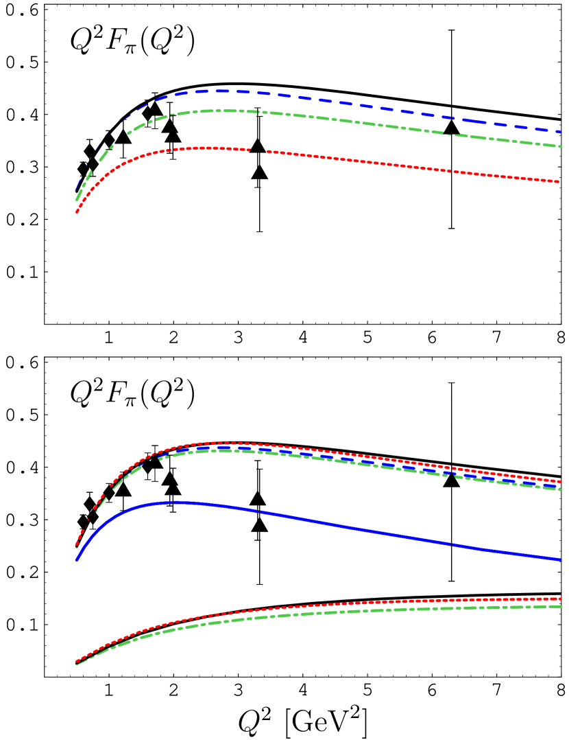
Figure 1: Predictions for $Q^{2}F_{\pi}(Q^{2})$ using APT and the BMS pion DA [4] in conjunction with the “Naive Analytic” (top) and “Maximally Analytic” (bottom) procedures [10]: $\overline{{\rm MS}}$ scheme and $\mu_{\rm R}^{2}=Q^{2}$ (dashed line); BLM (dotted line); $\overline{{\rm BLM}}$ (solid line); $\alpha_{V}$-scheme (dash-dotted line). The single solid line in the lower panel shows the prediction for the soft form-factor part; below this, the corresponding hard contributions are also displayed.

The analytization of $F_{\pi}^{\rm fact}(Q^{2})$ means to replace the running coupling and its powers by analytic expressions. We consider here two different analytization procedures in parity:
(i) Naive Analytization [2, 10] replaces in $F_{\pi}^{\rm fact}$ the strong coupling and its powers by the analytic coupling $\bar{\alpha}_{\rm s}$ [12] and its powers $\left[\bar{\alpha}_{\rm s}^{(N)}(\mu_{\rm R}^{2})\right]^{n}$, i.e.,

$$\mathbb{A}_{\rm naive}[\alpha_{\rm s}^{(N)n}(Q^{2})]=\bar{\alpha}_{\rm s}^{(N)n}(Q^{2})\,,$$ (5)

amounting at NLO to

$$\!\!\!\!\!\!\!\!\!\!\!\!\left[F_{\pi}^{\rm fact}(Q^{2};\mu_{\rm R}^{2})\right]_{\rm NaivAn}=\bar{\alpha}_{\rm s}^{(2)}(\mu_{\rm R}^{2})\,{\cal F}_{\pi}^{\rm LO}(Q^{2})$$ (6)

$$+\frac{1}{\pi}\,\left[\bar{\alpha}_{\rm s}^{(2)}(\mu_{\rm R}^{2})\right]^{2}\,{\cal F}_{\pi}^{\rm NLO}(Q^{2};\mu_{\rm R}^{2})\,.$$

(ii) Maximal Analytization [10] associates to the powers of the running coupling their own dispersive images, trading this way the usual power series expansion for a non-power functional expansion [12] to get

$$\mathbb{A}_{\rm max}[\alpha_{\rm s}^{(N)n}(Q^{2})]={\cal A}_{n}^{(N)}(Q^{2})\,,$$ (7)

where $N$ is the number of loops and $n$ the index of expansion. This entails at the two-loop level

$$\!\!\!\!\!\!\!\!\!\!\!\!\left[F_{\pi}^{\rm fact}(Q^{2};\mu_{\rm R}^{2})\right]_{\rm MaxAn}\ =\bar{\alpha}_{\rm s}^{(2)}(\mu_{\rm R}^{2})\,{\cal F}_{\pi}^{\rm LO}(Q^{2})$$ (8)

$$+\frac{1}{\pi}\,{\cal A}_{2}^{(2)}(\mu_{\rm R}^{2})\,{\cal F}_{\pi}^{\rm NLO}(Q^{2};\mu_{\rm R}^{2})\,,$$

with $\bar{\alpha}_{\rm s}^{(2)}$ and ${\cal A}_{2}^{(2)}(\mu_{\rm R}^{2})$ being the 2-loop analytic images of $\alpha_{\rm s}^{(2)}(Q^{2})$ and $\left(\alpha_{\rm s}^{(2)}(Q^{2})\right)^{2}$, respectively. Studying $F_{\pi}^{\rm fact}(Q^{2})$ beyond the LO requires an optimal renormalization scheme and scale setting in order to minimize the influence of higher-order loop corrections and avoid dependence of the results on the particular renormalization scheme and scales adopted. An in-depth analysis of these issues was carried out in [10], where estimates of $F_{\pi}^{\rm fact}(Q^{2})$ in conventional QCD perturbation theory within the $\overline{{\rm MS}}$ scheme with various scale settings were contrasted to analogous results obtained in APT. To confront these predictions with experimental data (Fig. 1), the soft nonfactorizable contribution was incorporated via local duality (LD) and the Ward identity at $Q^{2}=0$ was implemented by a power-behaved pre-factor in order to ensure that each of these two contributions was evaluated in its own momentum region of validity. Hence, we have

$$F_{\pi}(Q^{2};\mu_{\rm R}^{2})=F_{\pi}^{\rm LD}(Q^{2})+\hat{F}_{\pi}^{\rm fact}(Q^{2};\mu_{\rm R}^{2})$$ (9)

with

$$\hat{F}_{\pi}^{\rm fact}(Q^{2};\mu_{\rm R}^{2})=\left[\frac{Q^{2}}{2s_{0}^{\rm(2)}+Q^{2}}\right]^{2}\!F_{\pi}^{\rm fact}(Q^{2};\mu_{\rm R}^{2})$$ (10)

and $s_{0}^{(2)}\simeq 0.6$ GeV² (for more details, see [10]).

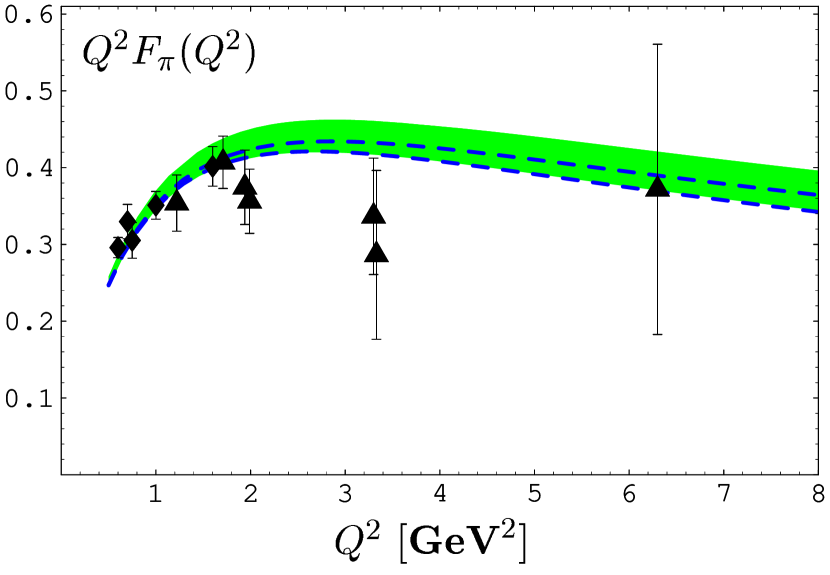
Figure 2: Predictions for $Q^{2}F_{\pi}(Q^{2})$ calculated with the “Maximally Analytic ” procedure and the pion DAs derived with nonlocal QCD sum rules [4] (shaded strip). The broken lines denote the region accessible to the asymptotic pion DA. The experimental data are taken from [7] (diamonds) and [16] (triangles).

The main phenomenological upshot of the presented analysis is shown in Fig. 2. It is interesting to observe from this figure that the theoretical error bounds (shaded strip) induced by the nonperturbative determination of the pion DA within the nonlocal QCD sum-rules picture are much smaller than those of the current high-momentum experimental data. This situation may, however, dramatically improve in a couple of years when the approved upgrade of CEBAF@JLab to an energy of $12$ GeV will start delivering high-precision data up to momentum transfers of about $6$ GeV² (see second entry in [7]). Another striking observation from this figure is that the form-factor predictions obtained with the double-humped BMS pion DA are only slightly larger than those following from the single-peaked asymptotic DA (area within the two broken lines). Hence, it becomes evident that what counts for the form factor is not the central region of longitudinal momenta around $x\simeq 1/2$ of the pion DA, but its endpoint regions $x\sim 0,1$ [4, 9, 10], as pointed out before in [2]. If the endpoint region is suppressed, then the form-factor prediction does not get artificial enhancement that may jeopardize the perturbative treatment. This suppression is controlled by the nonlocality of the scalar quark condensate, parameterized by the average quark virtuality $\lambda_{q}^{2}$ in the vacuum, with theoretical estimates in the range $(0.4-0.5)~{}\mbox{GeV}^{2}$ [17] and a preferable value of $0.4$ GeV² extracted in [9] from the CLEO data.

Figure 3: Predictions for the spacelike pion form factor including Sudakov effects within the Naive Analytization framework [2]. LO calculation—dash-dotted line; NLO result—dotted line; soft-overlap contribution—dashed line. The solid line represents the sum of the NLO hard contribution and the soft one.

Another means to suppress the endpoint region is provided by the Sudakov form factor [18] to which we now turn our attention. Sudakov resummation in conjunction with “Naive Analytization” was first considered in [2] in connection with the asymptotic pion DA and Fig. 3 shows the prediction for the form factor based on a NLO calculation similar to that in [10].

3 Conclusions

I have discussed a cutting-edge analysis [10] of the electromagnetic pion form factor, representing a confluence of advantages in QCD, ranging from non-power series fixed-order [12] and resummed analytic perturbation theory [2] to an improved CLEO data processing [8, 9] and to nonperturbative modelling of the pion distribution amplitude via nonlocal condensates [4]. It appears that the principle of Maximal Analytization [10] of hadronic observables in conjunction with QCD perturbation theory helps to offset the renormalization-scheme and scale-setting dependence—unavoidable in the conventional power-series perturbative expansion—already at NLO. The crucial observation on the nonperturbative side [9] is that the CLEO [6] and the CELLO [19] data on the pion-photon transition and also the JLab data [7] on the pion’s electromagnetic form factor can be best described by the doubly peaked but endpoint-suppressed BMS pion distribution amplitude [4] with all other known model distribution amplitudes being relatively disfavored by one or the other set of experimental data at least at the $2\sigma$ level [10, 20].

I am confident that the analytic perturbative approach presented here—to be seen in conjunction with several other applications discussed elsewhere [12]—is a key step towards achieving a better control over perturbative expansions, in particular, in the low $Q^{2}$ domain—especially after integrating more accurately resummation techniques under (Maximal) Analytization.

References

- [1] B. Melić, B. Nižić and K. Passek, Phys. Rev. D 60 (1999) 074004; ibid. D 65 (2002) 053020.
- [2] N.G. Stefanis, W. Schroers and H.C. Kim, Phys. Lett. B 449 (1999) 299; Eur. Phys. J. C 18 (2000) 137.
- [3] B. Melić, D. Müller and K. Passek-Kumerički, Phys. Rev. D 68 (2003) 014013.
- [4] A. P. Bakulev, S. V. Mikhailov and N.G. Stefanis, Phys. Lett. B 508 (2001) 279 [Erratum-ibid. B 590 (2004) 309].
- [5] A. Khodjamirian, Eur. Phys. J. C 6 (1999) 477; V.M. Braun, A. Khodjamirian and M. Maul, Phys. Rev. D 61 (2000) 073004; J. Bijnens and A. Khodjamirian, Eur. Phys. J. C 26 (2002) 67.
- [6] J. Gronberg et al., Phys. Rev. D 57 (1998) 33.
- [7] J. Volmer et al., Phys. Rev. Lett. 86 (2001) 1713; H.P. Blok, G.M. Huber and D.J. Mack, nucl-ex/0208011.
- [8] A. Schmedding and O.I. Yakovlev, Phys. Rev. D 62 (2000) 116002.
- [9] A.P. Bakulev, S.V. Mikhailov and N.G. Stefanis, Phys. Rev. D 67 (2003) 074012; Phys. Lett. B 578 (2004) 91.
- [10] A.P. Bakulev, K. Passek-Kumerički, W. Schroers and N.G. Stefanis, Phys. Rev. D 70 (2004) 033014.
- [11] Y.L. Dokshitzer, G. Marchesini and B.R. Webber, Nucl. Phys. B 469 (1996) 93.
- [12] D.V. Shirkov and I.L. Solovtsov, Phys. Rev. Lett. 79 (1997) 1209; Theor. Math. Phys. 120 (1999) 1220; D.V. Shirkov, Theor. Math. Phys. 127 (2001) 409; Eur. Phys. J. C 22 (2001) 331; hep-ph/0408272.
- [13] G. Grunberg, hep-ph/9705290.
- [14] A.I. Karanikas and N.G. Stefanis, Phys. Lett. B 504 (2001) 225; N.G. Stefanis, Lect. Notes Phys. 616 (2003) 153.
- [15] A.V. Efremov and A.V. Radyushkin, Phys. Lett. B 94 (1980) 245; Theor. Math. Phys. 42 (1980) 97; G.P. Lepage and S.J. Brodsky, Phys. Rev. D 22 (1980) 2157.
- [16] C.N. Brown et al., Phys. Rev. D 8 (1973) 92; C.J. Bebek et al., D 13 (1976) 25.
- [17] A.P. Bakulev and S.V. Mikhailov, Phys. Rev. D 65 (2002) 114511.
- [18] H.n. Li and G. Sterman, Nucl. Phys. B 381 (1992) 129.
- [19] H.J. Behrend et al., Z. Phys. C 49 (1991) 401.
- [20] A.P. Bakulev, S.V. Mikhailov and N.G. Stefanis, Ann. Phys. (Leipzig) 13 (2004) 629 [hep-ph/0410138].