QCD Green functions in a gluon field

Abstract:

We formulate a dressed perturbative expansion of QCD, where the standard diagrams are evaluated in the presence of a constant external gluon field whose magnitude is gaussian distributed. The approach is Poincaré and gauge invariant, and modifies the usual results for hard processes only by power suppressed contributions. Long distance propagation of quarks and gluons turns out to be inhibited due to a branch point singularity instead of a pole at $p^{2}=0$ in the quark and gluon propagators. The dressing keeps the (massless) quarks in ${\rm q}{\rm\bar{q}}\$ fluctuations of the photon at a finite distance from each other.

1 Introduction

The presence of a gluon and quark ‘condensate’ in the QCD ground state is a plausible reason for the observed long distance properties of QCD [1, 2]. The condensate apparently prevents quarks and gluons from propagating over long distances, while acting as a superfluid for color singlet hadrons. In this work we model the gluon condensate effects by coupling quarks and gluons to a ‘vacuum’ gluon field $\Phi$ which is taken as a constant in space-time in a covariant gauge. Translation invariance is thus automatically satisfied. We integrate over the Lorentz and color components of $\Phi_{\mu}^{a}$ with a gaussian weight. This ensures Lorentz and gauge invariance and introduces a dimensionful parameter $\Lambda$ which characterizes the magnitude of the vacuum field. In effect, we modify QCD perturbation theory (PQCD) by expanding around non-vanishing gluon field configurations.

In the limit of a large number of colors $N\to\infty$ with $g^{2}N$ fixed [3], we are able to find the exact expressions for the gluon and (massless) quark propagators in a ‘dressed tree’ approximation. The vacuum field effects are resummed to all orders, whereas perturbative loop corrections are neglected. The dressed tree propagators have a $1/\sqrt{p^{2}}$ branch cut instead of a pole at $p^{2}=0$, and consequently decay with time $t$ as $1/\sqrt{t}$. For $|p^{2}|\gg\mu^{2}=g^{2}N\Lambda^{2}$ the dressed propagators approach the free ones. Hence the short distance structure of PQCD is unaffected by the vacuum field. It is gratifying that the momentum dependence of our dressed quark and gluon propagators in the large $N$ limit turns out to agree qualitatively with the results of lattice calculations at $N=3$.

The finite propagation length of the dressed partons appears to regularize the infrared (IR) singularities of the standard PQCD expansion. We study the dressed (massless) quark loop contribution to the photon self-energy. Zero-momentum gluons can couple to the quark loop even for spacelike photons due to the appearance of infrared singularities in Feynman diagrams involving the coupling of at least $4$ external fields. While the contribution of a specific number of external fields is thus ill-defined, the loop integral is IR regular when the fully dressed quark propagator and quark-photon vertex are used. The effective lower cut-off for the loop momentum $k$ is $k^{2}\sim\mu^{2}=g^{2}N\Lambda^{2}$ (in euclidean space). Thus the dressing indeed ‘confines’ the color singlet quark pair within a distance $\sim 1/\mu$. At high photon virtualities $p^{2}$ the dressing correction is $\propto 1/p^{4}$ as in the QCD sum rule framework [1], where the normalization would be given by the vacuum expectation value $\langle{\alpha_{s}F^{a}_{\mu\nu}F_{a}^{\mu\nu}}\rangle$.

Since the elementary constituents of QCD are confined their Green functions need not have a standard analytic structure. Our dressed quark and gluon propagators indeed have branch cuts in $p^{2}$. The present framework may thus give insights into how an S-matrix consistent with general principles can be constructed in a confining theory. A first step in this direction will be to identify the asymptotic states of our framework.

This work represents a further development of our previous work [4], where some of the results on the dressed quark propagator and photon self-energy were already presented.

2 Coupling quarks and gluons to the vacuum field

Gauge invariant couplings of quarks and gluons to the vacuum field $\Phi$ can be found by shifting the gluon field,

$$A^{\mu}\to A^{\mu}+\Phi^{\mu}$$ (1)

The quark part $\bar{\psi}i\parbox[b]{10.00002pt}{$D$}\parbox[b]{8.00003pt}{ \raisebox{0.86108pt}{$/$}}\psi$ of the massless QCD lagrangian (with $D_{\mu}=\partial_{\mu}+igA_{\mu}$ the covariant derivative) then generates the coupling

$${\cal L}_{\Phi{\rm q}}=-g\bar{\psi}\Phi^{\mu}\gamma_{\mu}\psi$$ (2)

which we shall use. It is invariant under the gauge transformation $\psi\to U(x)\psi$ with $U(x)\in{\rm SU}(N)$ provided $\Phi$ transforms as

$$\Phi^{\mu}\to U(x)\Phi^{\mu}U(x)^{\dagger}$$ (3)

This transformation law is consistent with that of the shifted gluon field,

$$A^{\mu}+\Phi^{\mu}\to U(A^{\mu}+\Phi^{\mu})U^{\dagger}+\frac{i}{g}\left(\partial^{\mu}U\right)U^{\dagger}$$ (4)

Under the shift (1) the field strength tensor

$$F_{\mu\nu}=\partial_{\mu}A_{\nu}-\partial_{\nu}A_{\mu}+ig\left[{A_{\mu}},{A_{\nu}}\right]$$ (5)

becomes

$$F_{\mu\nu} \to F_{\mu\nu}+F^{\Phi}_{\mu\nu}+\Phi_{\mu\nu}$$ (6)

$$F^{\Phi}_{\mu\nu} = \partial_{\mu}\Phi_{\nu}-\partial_{\nu}\Phi_{\mu}+ig(\left[{\Phi_{\mu}},{A_{\nu}}\right]-\left[{\Phi_{\nu}},{A_{\mu}}\right])$$ (7)

$$\Phi_{\mu\nu} = ig\left[{\Phi_{\mu}},{\Phi_{\nu}}\right]$$ (8)

Since $F_{\mu\nu}\to UF_{\mu\nu}U^{\dagger}$ under a gauge transformation, each term in the r.h.s. of (6) of a given degree in $\Phi^{\mu}$ transforms similarly:

$$F_{\mu\nu}\to UF_{\mu\nu}U^{\dagger}\ \ ;\ \ F^{\Phi}_{\mu\nu}\to UF^{\Phi}_{\mu\nu}U^{\dagger}\ \ ;\ \ \Phi_{\mu\nu}\to U\Phi_{\mu\nu}U^{\dagger}$$ (9)

We wish to study the influence of a low-momentum ‘vacuum’ gluon field $\Phi$ on quark and gluon propagation without delving into the more difficult question of how the condensate field is generated. We therefore ignore the self-interactions of $\Phi$ and consider only the gauge invariant coupling of the $\Phi$ field to gluons which is linear in $\Phi$,

$${\cal L}_{\Phi{\rm g}}=-\mathrm{Tr}\,\left[F^{\mu\nu}F_{\mu\nu}^{\Phi}\right]$$ (10)

We shall thus work with the modified (massless) QCD lagrangian,

$${\cal L}=\bar{\psi}i\parbox[b]{10.00002pt}{$D$}\parbox[b]{8.00003pt}{ \raisebox{0.86108pt}{$/$}}\psi-\frac{1}{2}\mathrm{Tr}\,\left[F_{\mu\nu}F^{\mu\nu}\right]-\frac{1}{\xi}\mathrm{Tr}\,\left[(\partial_{\mu}A^{\mu})^{2}\right]-{\bar{c}}\,\partial^{\mu}D_{\mu}c-\lambda\,g\bar{\psi}\parbox[b]{10.00002pt}{$\Phi$}\parbox[b]{8.00003pt}{ \raisebox{0.86108pt}{$/$}}\psi-\mathrm{Tr}\,\left[F^{\mu\nu}F_{\mu\nu}^{\Phi}\right]$$ (11)

which includes covariant gauge fixing and ghost terms and is BRST invariant. Since the quark and gluon couplings to $\Phi$ are separately gauge invariant there is no constraint on their relative weight $\lambda$. For simplicity we choose $\lambda=1$ in the following.

As the field $\Phi$ is meant to describe the long wavelength (vacuum) effects we take it to carry zero momentum, i.e., to be independent of the coordinate $x$ (in the covariant gauge specified by (11)). Translation invariance is thus guaranteed. In order to preserve Lorentz (and gauge) invariance we average over all Lorentz (and color) components of $\Phi_{\mu}^{a}$ with a gaussian weight,

$$\left(\prod\,\int_{-\infty}^{\infty}d\Phi_{\mu}^{a}\right)\exp\left[\frac{1}{2\Lambda^{2}}\Phi_{\nu}^{b}\Phi^{\nu}_{b}\right]$$ (12)

where $\Lambda$ is a parameter with the dimension of mass. In a perturbative expansion we may interpret (12) as giving a $\Phi$ ‘propagator’

$$iD_{\Phi,\mu\nu}^{ab}(p)=-\Lambda^{2}g_{\mu\nu}\delta^{ab}(2\pi)^{4}\delta^{4}(p)$$ (13)

In the next section we derive explicit expressions for the quark and gluon propagators in a ‘dressed tree’ approximation, which takes all interactions with the $\Phi$ field into account, but neglects perturbative quark and gluon loops.

3 Dressed quark and gluon propagators in the large $N$ limit

We now calculate the effects of the interaction terms (2) and (10) of the zero-momentum vacuum field $\Phi$ on the quark and gluon propagators. We simplify the topology of the contributing diagrams by taking the limit of a large number of colors, $N\to\infty$ with $g^{2}N$ fixed [3]. In addition to the coupling $g^{2}N$ we have a parameter $\mu$ with the dimension of mass,

$$\mu^{2}=g^{2}N\,\Lambda^{2}$$ (14)

With the lagrangian (11) the full perturbative expansion of any quark and gluon Green function $G$ is a double sum of the form

$$G=\sum_{\ell=0}^{\infty}(g^{2}N)^{\ell}\sum_{k=0}^{\infty}C_{\ell,k}\ \mu^{2k}$$ (15)

Here $\ell$ counts the number of perturbative loops and $2k$ the number of $\Phi$ couplings (2) or (10). We evaluate the complete sum over $k$ for $\ell=0$. This is possible since the $\Phi$ propagator (13) carries zero momentum so no loop integrals are involved. The remaining sum over $\ell$ involves higher powers of the coupling $g^{2}N$ and an increasing number of non-trivial loop integrals.

3.1 Dressed quark propagator

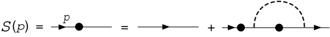
Figure 1: Implicit equation for the dressed quark propagator $S(p)$. The dashed line denotes the $\Phi$ ‘propagator’ (2.13).

Only planar $\Phi$ ‘loop’ corrections to the free quark propagator contribute in the large $N$ limit (with $\ell=0$ in (15)). From the structure of a general diagram it is readily seen that the dressed quark propagator $S(p)$ satisfies the Dyson-Schwinger (DS) type equation shown in Fig. 1, which reads

$$iS(p) = \frac{i}{\parbox[b]{6.00006pt}{$p$}\parbox[b]{5.50003pt}{ \raisebox{-0.86108pt}{$/$}}}+C_{F}(-ig)^{2}(-\Lambda^{2})\frac{i}{\parbox[b]{6.00006pt}{$p$}\parbox[b]{5.50003pt}{ \raisebox{-0.86108pt}{$/$}}}\gamma^{\mu}iS(p)\gamma_{\mu}iS(p)$$

$$\Rightarrow\ \ \parbox[b]{6.00006pt}{$p$}\parbox[b]{5.50003pt}{ \raisebox{-0.86108pt}{$/$}}S(p)=1-{\textstyle\frac{1}{2}}\mu^{2}\,\gamma^{\mu}S(p)\gamma_{\mu}S(p)$$ (16)

where $\mu$ is defined in (14) and we used $C_{F}=N/2$ at leading order in $N$. The DS equation (16) generates all one-particle irreducible as well as reducible planar diagrams.

Lorentz invariance constrains the quark propagator to be of the form

$$S(p)=a_{p}\,\parbox[b]{6.00006pt}{$p$}\parbox[b]{5.50003pt}{ \raisebox{-0.86108pt}{$/$}}+b_{p}$$ (17)

where $a_{p}$ and $b_{p}$ are functions of $p^{2}$. Substituting this in (16) we get

$$b(1+\mu^{2}a)=0\ \ {\rm and}\ \ ap^{2}(1-\mu^{2}a)=1-2\mu^{2}b^{2}$$ (18)

A chiral symmetry conserving quark propagator $S_{1}(p)$ must have $b=0$. The second order equation for $a$ then gives

$$a_{p} = \frac{1}{2\mu^{2}}\left(1-\sqrt{1-\frac{4\mu^{2}}{p^{2}}}\right)$$ (19)

$$S_{1}(p) = \frac{2\parbox[b]{6.00006pt}{$p$}\parbox[b]{5.50003pt}{ \raisebox{-0.86108pt}{$/$}}}{p^{2}+\sqrt{p^{2}(p^{2}-4\mu^{2})}}$$ (20)

where we chose the sign of the square root so as to ensure that the propagator approaches the free one in the $p^{2}\to\infty$ limit:

$$S_{1}(p)=\frac{1}{\parbox[b]{6.00006pt}{$p$}\parbox[b]{5.50003pt}{ \raisebox{-0.86108pt}{$/$}}}\left[1+{\cal O}\left(\frac{\mu^{2}}{p^{2}}\right)\right]\ \ \ {\rm for}\ \ p^{2}\to\infty$$ (21)

The $p^{2}=0$ pole of the free quark propagator $\parbox[b]{6.00006pt}{$p$}\parbox[b]{5.50003pt}{ \raisebox{-0.86108pt}{$/$}}/p^{2}$ has been removed by the dressing. The dressed propagator $S_{1}(p)$ given in (20) has instead branch point singularities at $p^{2}=0$ and $p^{2}=4\mu^{2}$. In appendix A (see (67)) we show that this removes the quark from the set of asymptotic states, in the sense that the Fourier transformed propagator vanishes at large times,

$$|S_{1}(t,{\bf p})|\ \ \mathop{\sim}_{|t|\to\infty}\ \ {\cal O}\left(1/\sqrt{|t|}\right)$$ (22)

Allowing chiral symmetry breaking ($\chi$${\textstyle SB}$), i.e., $b\neq 0$ in (18) we find

$$S_{2}(p)=-\frac{1}{\mu^{2}}\left(\parbox[b]{6.00006pt}{$p$}\parbox[b]{5.50003pt}{ \raisebox{-0.86108pt}{$/$}}\pm\sqrt{p^{2}+\mu^{2}/2}\right)=\frac{1}{2(\parbox[b]{6.00006pt}{$p$}\parbox[b]{5.50003pt}{ \raisebox{-0.86108pt}{$/$}}\mp\sqrt{p^{2}+\mu^{2}/2})}$$ (23)

This solution is singular for $\mu^{2}\to 0$ and hence does not have a power expansion in $\mu^{2}$ of the form (15). It emerges as a ‘non-perturbative’ solution of the implicit equation (16). Like the chiral symmetry conserving solution $S_{1}$, the propagator $S_{2}$ has no quark pole, only a branch point at $p^{2}=-\mu^{2}/2$, where it coincides with $S_{1}$. Since the solution $S_{2}(p)$ does not approach the perturbative propagator $1/\parbox[b]{6.00006pt}{$p$}\parbox[b]{5.50003pt}{ \raisebox{-0.86108pt}{$/$}}\$ at large $p^{2}$ it must be discarded at short distance.

In Euclidean space we can estimate the chiral symmetry breaking effect of using the solution $S_{2}(p_{E})$ for $0\leq p_{E}^{2}=-p^{2}\leq\mu^{2}/2$ and the $S_{1}$ propagator for $p_{E}^{2}>\mu^{2}/2$. The value of the quark condensate obtained in this way (using the upper sign in (23)) is

$$\langle{\bar{\psi}\psi}\rangle=\int\frac{d^{4}p_{E}}{(2\pi)^{4}}\,\mathrm{Tr}\,\left[S_{2}(p_{E})\right]\Theta(\mu^{2}/2-p_{E}^{2})=-\frac{\mu^{3}}{60\,\pi^{2}\sqrt{2}}$$ (24)

This estimate, ${\langle{\bar{\psi}\psi}\rangle}^{1/3}\simeq-\mu/9.4$, is an order of magnitude below the generic scale $\mu$.

Figure 2: Numerical results for the quark propagator in the euclidean region $p_{E}^{2}\equiv-p^{2}>0$. The quantities $M$ and $Z$ are defined in (3.12).

Expressing the quark propagator as

$$S(p)=\frac{Z(p^{2})}{\parbox[b]{6.00006pt}{$p$}\parbox[b]{5.50003pt}{ \raisebox{-0.86108pt}{$/$}}-M(p^{2})}$$ (25)

we plot in Fig. 2 the functions $M(p^{2})$ and $Z(p^{2})$, using $\mu=500\,\rm{MeV}$ and the above combination of $S_{1}$ and $S_{2}$ in the euclidean $p^{2}<0$ region. Their shapes are similar to the results obtained in lattice calculations, see for instance Refs. [2] or Fig. 3 of Ref. [5].

Let us mention that the above solutions $S_{1}$ and $S_{2}$ for the quark propagator were previously obtained in a different framework [6], and recently within a model assuming the presence of an $\langle{A_{\mu}^{a}A^{\mu}_{a}}\rangle$ condensate [7]. In the rest of this paper we shall use $S(p)=S_{1}(p)$ for all values of $p^{2}$.

3.2 Dressed gluon propagator

It is convenient to use the double line color notation [3] for the fields $A^{\mu}$ and $\Phi^{\mu}$ in the limit $N\to\infty$. The doubly indexed fields are defined in terms of the color generator matrices $T^{a}$ of the fundamental representation as

$${A^{\mu}}{{}_{i}^{\ {j}}\,}=A^{\mu a}T^{a}{{}_{i}^{\ {j}}\,}$$ (26)

In the covariant gauge defined by (11) the free propagators and their graphical representations are then

$$iD_{0}^{\mu\nu}(p){{}_{i}^{\ {j}}\,}{{}_{k}^{\ {l}}\,} = \ \ \ \mbox{\raisebox{-11.38092pt}{\hbox{\epsfbox{gluonprop.eps}}}}\ \ \ =\frac{1}{2}\delta{{}_{i}^{\ {l}}\,}\delta{{}_{k}^{\ {j}}\,}\,\frac{-i}{p^{2}}\left[g^{\mu\nu}-(1-\xi)\frac{p^{\mu}p^{\nu}}{p^{2}}\right]$$ (27)

$$iD_{\Phi}^{\mu\nu}(p){{}_{i}^{\ {j}}\,}{{}_{k}^{\ {l}}\,} = \ \ \ \mbox{\raisebox{-11.38092pt}{\hbox{\epsfbox{phiprop.eps}}}}\ \ \ =-\frac{1}{2}\delta{{}_{i}^{\ {l}}\,}\delta{{}_{k}^{\ {j}}\,}\,\Lambda^{2}g^{\mu\nu}\,(2\pi)^{4}\delta^{4}(p)$$ (28)

The interaction term (10) couples $\Phi$ to two and three gluons, via $\Phi AA$ and $\Phi AAA$ vertices, respectively. The $\Phi AAA$ vertex does not, however, contribute in the dressed tree approximation (the $\ell=0$ term in (15)), since it implies at least one perturbative loop integral. The $\Phi AA$ vertex is

$${\cal L}_{\Phi AA} = -2ig\mathrm{Tr}\,\big{(}\left[{\Phi_{\mu}},{A_{\nu}}\right](\partial^{\mu}A^{\nu}-\partial^{\nu}A^{\mu})\big{)}$$ (29)

$$= -2ig\mathrm{Tr}\,\big{(}\Phi_{\mu}\left[{A_{\nu}},{\partial^{\mu}A^{\nu}}\right]-\Phi_{\mu}\left[{A^{\mu}},{\partial^{\nu}A_{\nu}}\right]\big{)}$$

where we used $\partial_{\mu}\Phi_{\nu}=0$ and dropped a total derivative to obtain the second line. The second term of (29) vanishes in Landau gauge, $\partial^{\nu}A_{\nu}=0$. However, we keep both terms in order to see the dependence on the gauge parameter $\xi$. In the double line notation the corresponding Feynman rules are:

$$= \ -4ig\,p_{\mu}\,g_{\nu\rho}\,\delta{{}_{j}^{\ {k}}\,}\delta{{}_{l}^{\ {m}}\,}\delta{{}_{n}^{\ {i}}\,}$$ (30)

$$= \ +4ig\,p_{\rho}\,g_{\mu\nu}\,\delta{{}_{j}^{\ {k}}\,}\delta{{}_{l}^{\ {m}}\,}\delta{{}_{n}^{\ {i}}\,}$$ (31)

The rules for vertices where the $\Phi$ field attaches to the lower gluon color line are the same (up to an overall sign). Since nonplanar diagrams like the one shown in Fig. 3a do not contribute at large $N$, the $\Phi$ lines never cross the gluon propagator. A generic diagram contributing to our dressed tree approximation is shown in Fig. 3b.

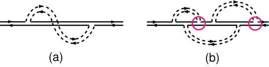
Figure 3: Diagrams contributing to the gluon propagator in the double line color notation: a non-planar subleading contribution (a) and a generic dominant contribution (b) in the large $N$ limit.

One might expect that the dressed tree gluon propagator would satisfy a DS equation (or a finite set of equations) analogous to the one satisfied by the dressed quark propagator (Fig. 1). However, because planar corrections to the gluon propagator can appear on both sides of the gluon line the dressed $\Phi gg$ vertex is not proportional to the bare vertex, as is the case for the quark. This apparently precludes a finite set of closed DS equations for the gluon propagator (which in our approach would imply an algebraic solution). By explicitly summing all diagrams we indeed find the non-algebraic expression (36) below.

We first do the calculation in Landau gauge ($\xi=0$), and then evaluate the $\xi$ dependence. In Landau gauge the free gluon propagator is transverse,

$$iD_{0}^{\mu\nu}(p){{}_{i}^{\ {j}}\,}{{}_{k}^{\ {l}}\,}=\frac{1}{2}\delta{{}_{i}^{\ {l}}\,}\delta{{}_{k}^{\ {j}}\,}\,\frac{-i}{p^{2}}\,P_{T}^{\mu\nu}(p)\ \ ;\ \ P_{T}^{\mu\nu}(p)=g^{\mu\nu}-\frac{p^{\mu}p^{\nu}}{p^{2}}$$ (32)

and thus the circled vertex (31) does not contribute. Independently of the topology of a diagram, adding one $\Phi$ (double) line always yields the same factor, namely,

$$N(-4ig)^{2}p^{2}\left(\frac{-\Lambda^{2}}{2}\right)\left(\frac{-i}{2p^{2}}\right)^{2}=-\frac{2\mu^{2}}{p^{2}}\equiv x$$ (33)

Let $n(k)$ be the number of distinct planar graphs having $k$ $\Phi$ lines (cf. (15)). The dressed gluon propagator in Landau gauge is then (with standard gluon color indices):

$$iD^{\mu\nu}_{ab}(p)=\frac{-i}{p^{2}}\,P_{T}^{\mu\nu}(p)\,d\left(-\frac{2\mu^{2}}{p^{2}}\right)\delta_{ab}\ \ \ {\rm with}\ \ \ d(x)=\sum_{k=0}^{\infty}n(k)\,x^{k}\,.$$ (34)

In appendix B we show that $n(k)=C_{k}\,C_{k+1}$, where $C_{k}$ is a Catalan number (see (79) and (80)). Mathematica then gives for the ‘gluon polarization function’ $d(x)$:

$$d(x)=\sum_{k=0}^{\infty}C_{k}\,C_{k+1}\,x^{k}=\frac{1-h(16x)}{2x}\ \ \ {\rm with}\ \ \ h(x)={{}_{2}F}_{1}\left(-\frac{1}{2},\frac{1}{2},2,x\right)\,.$$ (35)

The dressed gluon propagator is thus, in Landau gauge,

$$iD^{\mu\nu}_{ab}(p)=\frac{i}{4\mu^{2}}\,P_{T}^{\mu\nu}(p)\,\left[1-{{}_{2}F}_{1}\left(-\frac{1}{2},\frac{1}{2},2,-\frac{32\mu^{2}}{p^{2}}\right)\right]\delta_{ab}$$ (36)

From the integral representation of the hypergeometric function $h(x)$,

$$h(x)=\frac{4}{\pi}\int_{0}^{1}du\,\sqrt{1-u^{2}}\,\sqrt{1-x\,u^{2}}$$ (37)

we see that $h(x)$ has a branch cut for $x\geq 1$. This implies that the gluon propagator (36) has a cut for

$$-32\mu^{2}\leq p^{2}\leq 0\,,$$ (38)

which, surprisingly, lies in the spacelike $p^{2}<0$ region.

The polarization function $d(x)$ approaches unity in the limit of high gluon virtuality, $x=-2\mu^{2}/p^{2}\to 0$:

$$d(x\to 0)=1+2x+10x^{2}+{\cal O}\left(x^{3}\right)$$ (39)

Thus the dressing effects are power suppressed at short distances, as expected. In the long distance limit $p^{2}\to 0$ ($x\to\infty$) the function $d(x)$ vanishes,

$$d(x\to+\infty)=\frac{8}{3\pi}\,\frac{1}{\sqrt{-x}}+\frac{1}{2x}+{\cal O}\left(\frac{1}{x\sqrt{x}}\right)$$ (40)

which turns the $p^{2}=0$ pole of the free propagator into a $1/\sqrt{p^{2}}$ singularity. As for the quark, this implies that the gluon propagator decays with time $t$ as $1/\sqrt{t}$, see (68) of Appendix A.

We plot $d(-2\mu^{2}/p^{2})$ for $p^{2}<0$ and $\mu=500\,{\rm MeV}$ in Fig. 4. The real part has a shape similar to the gluon propagator found numerically in a Landau gauge lattice calculation, see Refs. [2] or Fig. 3 of Ref. [8]. However, the presence in our expression (36) of a branch cut in the euclidean region $p^{2}<0$ gives a negative imaginary part to the polarization function which obscures the comparison.

Figure 4: Real part (solid line) and absolute value of the imaginary part (dashed line) of the gluon polarization function $d(x)$ in the euclidean region $p_{E}^{2}\equiv-p^{2}>0$.

Our result (35) for the polarization function $d(-2\mu^{2}/p^{2})$ was derived in Landau gauge ($\xi=0$ in (27)). We now show that this expression actually is independent of $\xi$, i.e., the dressed gluon propagator in a general covariant gauge is

$$iD^{\mu\nu}_{ab}(p)=\frac{-i}{p^{2}}\,\left[P_{T}^{\mu\nu}(p)\,d\left(-\frac{2\mu^{2}}{p^{2}}\right)+\xi\frac{p^{\mu}p^{\nu}}{p^{2}}\right]\,\delta_{ab}$$ (41)

The $\xi$-independence of $d(x)$ actually holds separately for any diagram contributing to $d(x)$, planar or non-planar. This can be seen as follows, using the standard single line color notation for the gluon and $\Phi$ propagators. Let $k$ be the number of $\Phi$-lines of a diagram with given topology. Since the free gluon propagator has a longitudinal part $\propto\xi$,

$$iD_{0,ab}^{\mu\nu}(p)=\frac{-i}{p^{2}}\,\left(P_{T}^{\mu\nu}(p)+\xi P_{L}^{\mu\nu}(p)\right)\,\delta_{ab}\ \ ;\ \ P_{L}^{\mu\nu}(p)=\frac{p^{\mu}p^{\nu}}{p^{2}}$$ (42)

the circled vertex (31) can contribute when $\xi\neq 0$. There are $2^{2k}$ contributions for a given topology, since a chosen vertex can be either circled or not. When no vertex is circled the Lorentz structure brought by the gluon line is $\propto(P_{T}+\xi P_{L})^{2k+1}=P_{T}+\xi^{2k+1}P_{L}$. When at least one vertex is circled, consider the first vertex of this type one meets by following the gluon line (carrying momentum $p$) from left to right. In all gluon propagators to the right of this vertex only the longitudinal part $P_{L}$ contributes. The $m$ gluon propagators to the left of this vertex give $(P_{T}+\xi P_{L})^{m}=P_{T}+\xi^{m}P_{L}$, i.e. these $m$ propagators are of the same type, either transverse or longitudinal. Independently of the topological configuration, $(P_{T}+\xi^{m}P_{L})^{\mu\nu^{\prime}}$ is always contracted with $p_{\nu^{\prime}}$ ($\nu^{\prime}$ being the Lorentz index of the gluon line just before the first circled vertex). As a result, in all $(2k+1)$ gluon propagators, only the longitudinal part contributes when at least one among the $2k$ vertices is circled. Since the circled vertex has a negative sign relative to the uncircled one, the $\xi$-dependent part brought by the $2^{2k}$ contributions is proportional to:

$$\xi^{2k+1}P_{L}\sum_{n=0}^{2k}(-1)^{n}{2k\choose n}=0$$ (43)

Only the $\xi$-independent (transverse) contribution remains, which is obtained when no vertex is circled. Thus the result found in Landau gauge for $k\geq 1$ holds in all covariant gauges, establishing (41).

4 Photon self-energy

In the previous section we saw that the dressed quark and gluon propagators have no pole at $p^{2}=0$, only a $1/\sqrt{p^{2}}$ type singularity. This implies a limited propagation length and should soften the collinear $(p^{2}\to 0)$ and infrared ($p\to 0$) singularities of the perturbative expansion. In this section we study the effects of dressing the quark loop contribution to the self-energy of the photon.

4.1 Coupling of zero-momentum gluons to a color singlet quark loop

Spacelike photon fluctuations $\gamma(p)\to{\rm q}{\rm\bar{q}}\ \to\gamma(p)$ involve quark pairs of size $\sim 1/\sqrt{-p^{2}}$ (for massless quarks). One might expect that such compact, short-lived color singlet states would decouple from gluons of zero momentum, i.e., from the $\Phi$ field we introduced in section 2. This charge coherence effect is most easily seen for QED amplitudes. The standard contribution of a bare electron loop to the photon self-energy is

$$\Pi^{\alpha\beta}(p)=ie^{2}\int\frac{d^{d}k}{(2\pi)^{d}}{\rm Tr}\left[\gamma^{\beta}S_{e}(k)\gamma^{\alpha}S_{e}(\bar{k})\right]$$ (44)

where $\bar{k}=k-p$. It is instructive to retain the mass in the electron propagator

$$S_{e}(k)=\frac{1}{\parbox[b]{6.00006pt}{$k$}\parbox[b]{5.50003pt}{ \raisebox{-0.86108pt}{$/$}}-m}$$ (45)

Now consider the attachment of an external zero-momentum photon with Lorentz index $\mu_{1}$ to this loop. This contribution, denoted by $\Pi_{\mu_{1}}^{\alpha\beta}(p)$, is given by two diagrams. Using the identity

$$-\frac{\partial}{\partial k^{\mu_{1}}}\left(\frac{1}{\parbox[b]{6.00006pt}{$k$}\parbox[b]{5.50003pt}{ \raisebox{-0.86108pt}{$/$}}-m}\right)=\frac{1}{\parbox[b]{6.00006pt}{$k$}\parbox[b]{5.50003pt}{ \raisebox{-0.86108pt}{$/$}}-m}\,\gamma_{\mu_{1}}\,\frac{1}{\parbox[b]{6.00006pt}{$k$}\parbox[b]{5.50003pt}{ \raisebox{-0.86108pt}{$/$}}-m}$$ (46)

we note that $\Pi_{\mu_{1}}^{\alpha\beta}(p)$ is obtained from (44) by differentiating the integrand with respect to $k^{\mu_{1}}$,

$$\Pi_{\mu_{1}}^{\alpha\beta}(p)=ie^{2}\int\frac{d^{d}k}{(2\pi)^{d}}\,\left[-e\frac{\partial}{\partial k^{\mu_{1}}}\right]\,{\rm Tr}\left[\gamma^{\beta}S_{e}(k)\gamma^{\alpha}S_{e}(\bar{k})\right]$$ (47)

Similarly, the QED amplitude for an electron loop with two external zero-momentum photons is

$$\Pi_{\mu_{1}\mu_{2}}^{\alpha\beta}(p)=ie^{2}\int\frac{d^{d}k}{(2\pi)^{d}}\,\left[-e\frac{\partial}{\partial k^{\mu_{1}}}\right]\,\left[-e\frac{\partial}{\partial k^{\mu_{2}}}\right]\,{\rm Tr}\left[\gamma^{\beta}S_{e}(k)\gamma^{\alpha}S_{e}(\bar{k})\right]$$ (48)

In Eqs. (47) and (48) the integrand is given by a total derivative. This generalizes to any number of external zero-momentum photons. Thus the loop integral formally vanishes, in agreement with intuition that zero-momentum photons do not couple to a virtual $e^{+}e^{-}$ pair in a photon. The analogous proof for QCD is somewhat more involved and is given in Appendix C.

However, this demonstration fails if the integral is singular and thus ill-defined. As seen from (46) the insertion of a zero-momentum photon increases the number of electron propagators having the same momentum, which may cause infrared singularities. Consider the photon self-energy contribution with $n$ zero-momentum photons attached to a (massive) electron loop. In this amplitude there are diagrams with up to $n+1$ electron propagators of the same momentum, e.g., $[1/(\parbox[b]{6.00006pt}{$k$}\parbox[b]{5.50003pt}{ \raisebox{-0.86108pt}{$/$}}-m)]^{n+1}$. After a Wick rotation the integral has contributions at low $k$ of the form (for even $n$)

$$A_{n}\sim\int d^{4}k\,k^{n}\,\frac{k\cdot\bar{k}}{(k^{2}+m^{2})^{n+1}}$$ (49)

For a finite electron mass $m\neq 0$ the integrand is always regular at $k=0$ and, being a total derivative, the loop integral must indeed vanish. On the other hand, for $m=0$ the integral is apparently IR regular only for $n\leq 2$ (and thus vanishes for $n=2$ when the UV behaviour is dimensionally regularized). For $n\geq 4$ the loop integral is IR singular and hence ill-defined.

The physical reason for this infrared behaviour is that the coupling of a photon to an $e^{+}e^{-}$ pair is proportional to the electric dipole moment of the pair, which favors large dipole configurations in the integrand. For $n\geq 4$ the integral becomes divergent at $k=0$. The electron is then delocalized in space and by the uncertainty principle the pair can have any size. At $k=p$ the positron is similarly delocalized. This long-distance behaviour is a physical effect which cannot (or should not) be removed, e.g., using dimensional regularization. In the case of a finite electron mass the maximum size of the virtual pair is set by $1/m$ and no infrared singularities occur.

This analysis also applies to QCD. Zero-momentum gluons can couple to virtual ${\rm q}{\rm\bar{q}}\$ states in the photon and the dressing affects the photon self-energy. Using our dressed (chirally symmetric) quark propagator (20), and the dressed $\gamma{\rm q}{\rm\bar{q}}\$ vertex which we shall next derive, we find an infrared regular loop integral. The dressing thus keeps the quark pair at a finite separation $\sim 1/\mu$. Singularities only appear if one tries to Taylor expand in powers of $\mu^{2}$, implying that non-analytic terms in $\mu^{2}$ appear in a $\mu\to 0$ expansion.

4.2 Dressed quark-photon vertex

In our dressed tree approximation ($\ell=0$ in (15)) the $\gamma{\rm q}{\rm\bar{q}}\$ vertex $\Gamma^{\mu}(k,\bar{k})$ satisfies (at large $N$) the implicit equation of Fig. 5,

$$\Gamma^{\mu}(k,\bar{k})=\gamma^{\mu}-{\textstyle\frac{1}{2}}\mu^{2}\gamma^{\rho}S(k)\Gamma^{\mu}(k,\bar{k})S(\bar{k})\gamma_{\rho}$$ (50)

where ${\bar{k}}=k-p$ and $p$ is the photon momentum. When the vertex is expanded on its independent Dirac components (50) reduces to a set of linear equations for the components (cf. Eqs. (96) and (D)), with a unique solution when the quark propagator $S$ is given. The explicit expression (101) for $\Gamma^{\mu}(k,\bar{k})$ is derived in Appendix D using the chiral symmetry conserving quark propagator (20).

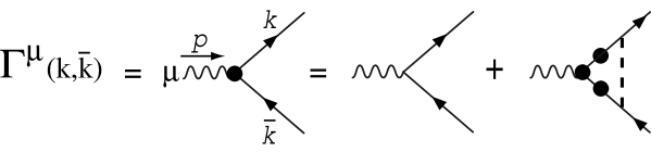
Figure 5: Implicit equation for the quark-photon vertex $\Gamma^{\mu}(k,\bar{k})$.

Multiplying (50) by $p_{\mu}=(k-\bar{k})_{\mu}$ and rewriting (16) as

$${\textstyle\frac{1}{2}}\mu^{2}\gamma^{\mu}S(k)\gamma_{\mu}=S(k)^{-1}-\parbox[b]{6.00006pt}{$k$}\parbox[b]{5.50003pt}{ \raisebox{-0.86108pt}{$/$}}$$ (51)

it is readily verified that the solution of (50) respects the Ward-Takahashi identity

$$p_{\mu}\Gamma^{\mu}(k,\bar{k})=S(k)^{-1}-S(\bar{k})^{-1}$$ (52)

For highly virtual momenta $k^{2}\to\infty$ (at fixed $p$), we have $S(k)\to 1/\parbox[b]{6.00006pt}{$k$}\parbox[b]{5.50003pt}{ \raisebox{-0.86108pt}{$/$}}$, $S(\bar{k})\to 1/\parbox[b]{6.00006pt}{$\bar{k}$}\parbox[b]{5.50003pt}{ \raisebox{-0.86108pt}{$/$}}$ and (50) thus implies

$$k^{2}\to\infty\ \ \Rightarrow\ \ \Gamma^{\mu}(k,\bar{k})=\gamma^{\mu}+{\cal O}\left(\frac{\mu^{2}}{k^{2}}\right)$$ (53)

This may also be verified from the explicit expression (101) of the dressed vertex.

4.3 Dressed quark loop

The dressed quark loop correction to the photon propagator is given by the dressed quark propagator and quark-photon vertex as indicated in Fig. 6. In terms of the solutions of the DS equations for the quark propagator (16) and vertex (50) the photon self-energy correction $\Pi^{\mu\nu}(p)$ is

$$\Pi^{\mu\nu}(p) = ie^{2}N\int\frac{d^{d}k}{(2\pi)^{d}}{\rm Tr}\left[\gamma^{\nu}S(k)\Gamma^{\mu}(k,\bar{k})S(\bar{k})\right]$$ (54)

$$= \frac{2}{d-2}\frac{ie^{2}N}{\mu^{2}}\int\frac{d^{d}k}{(2\pi)^{d}}\Big{\{}\mathrm{Tr}\,[(\Gamma^{\mu}(k,\bar{k})-\gamma^{\mu})\gamma^{\nu}]\Big{\}}$$ (55)

where we used the relation (50) for the vertex and $\gamma^{\nu}=\gamma_{\rho}\gamma^{\nu}\gamma^{\rho}/(2-d)$ in $d$ dimensions.

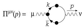
Figure 6: Photon self-energy $\Pi^{\mu\nu}(p)$ dressed by the $\Phi$ field. The dressed propagators and vertex are indicated by a solid circle.

We dimensionally regularize the standard ultraviolet divergence which appears at zeroth order in $\mu^{2}$. At ${\cal O}\left(\mu^{2}\right)$ the quark loop couples to two photons and two $\Phi$ fields and is UV finite, but is still ill-defined in $d=4$ because of the superficial logarithmic divergence of the loop integral. Due to (48) it vanishes when dimensionally regularized.

As is well-known, within dimensional regularization the Ward-Takahashi identity (52) implies a transverse photon self-energy

$$\Pi^{\mu\nu}(p)=\Pi(p^{2})\,(p^{2}g^{\mu\nu}-p^{\mu}p^{\nu})$$ (56)

and a resummed photon propagator

$$D_{\gamma}^{\mu\nu}(p)=\frac{1}{p^{2}[1-\Pi(p^{2})]}\left(-g^{\mu\nu}+\frac{p^{\mu}p^{\nu}}{p^{2}}\right)$$ (57)

where $p^{2}\,\Pi(p^{2})\to 0$ for $p^{2}\to 0$.

4.4 The dressed photon self-energy in euclidean space

Here we consider in more detail the expression for $\Pi(p^{2})$, specified by (55) and (56), using the quark propagator $S_{1}(p)$ given in (20) and the quark-photon vertex (101). To avoid UV divergent terms in the loop integral we subtract the terms of ${\cal O}\left(\mu^{0}\right)$ (i.e., the standard PQCD expression) and ${\cal O}\left(\mu^{2}\right)$ (which vanishes in dimensional regularization):

$${\widehat{\Pi}}(p^{2}) \equiv \Pi(p^{2})-\left.\Pi(p^{2})\right|_{\mu^{0}}-\left.\Pi(p^{2})\right|_{\mu^{2}}$$

$$= \frac{8ie^{2}N}{3p^{2}}\int\frac{d^{4}k}{(2\pi)^{4}}\left\{\frac{\mu^{2}k^{2}{\bar{k}}^{2}a_{k}^{2}a_{\bar{k}}^{2}}{1-\mu^{4}k^{2}{\bar{k}}^{2}a_{k}^{2}a_{\bar{k}}^{2}}-\frac{k\cdot\bar{k}\,a_{k}a_{\bar{k}}+\mu^{2}k^{2}{\bar{k}}^{2}a_{k}^{2}a_{\bar{k}}^{2}}{1+2\mu^{2}k\cdot\bar{k}a_{k}a_{\bar{k}}+\mu^{4}k^{2}{\bar{k}}^{2}a_{k}^{2}a_{\bar{k}}^{2}}\right.\ \$$

$$\hskip 199.16928pt+\left.\frac{k\cdot\bar{k}}{k^{2}{\bar{k}}^{2}}+\mu^{2}\frac{k\cdot\bar{k}}{k^{4}{\bar{k}}^{4}}\,p^{2}\right\}$$

where the function $a_{p}$ is given in (19).

${\widehat{\Pi}}(p^{2})$ has a complicated analytic structure due to the denominators of the integrand and the square roots in $a_{k}$ and $a_{\bar{k}}$. We shall here only address its properties for euclidean momenta $p^{2}<0$, assuming that the loop integral can be Wick rotated.

The denominator of the second term in the integrand of (4.4) can be estimated using $|k\cdot\bar{k}|\leq|k|\,|\bar{k}|$,

$$1-2\mu^{2}k\cdot\bar{k}a_{k}a_{\bar{k}}+\mu^{4}k^{2}{\bar{k}}^{2}a_{k}^{2}a_{\bar{k}}^{2}\geq\left(1-\mu^{2}|k|\,|\bar{k}|a_{k}a_{\bar{k}}\right)^{2}\geq 0$$ (59)

where we reversed the sign of all dot products since the momenta are now understood to be euclidean. This denominator can thus vanish only if

$$\mu^{4}k^{2}{\bar{k}}^{2}a_{k}^{2}a_{\bar{k}}^{2}=1$$ (60)

which is also the condition for the denominator of the first term in (4.4) to vanish. For euclidean $k^{2}>0$ the function $a_{k}$ is negative,

$$a_{k}=\frac{1}{2\mu^{2}}\left(1-\sqrt{1+\frac{4\mu^{2}}{k^{2}}}\right)<0$$ (61)

The identity

$$\mu^{2}a_{k}^{2}k^{2}=1+k^{2}a_{k}$$ (62)

then shows that $\mu^{2}a_{k}^{2}k^{2}<1$ (with a similar relation for $\bar{k}$). Consequently the condition (60) cannot be fulfilled for finite euclidean momenta, and the denominators in the expression (4.4) for $\widehat{\Pi}$ are positive definite.

It is remarkable that the loop integral in (4.4) is IR convergent. For $k\to 0$, we have $\bar{k}\to-p$ and $a_{k}\sim-1/\mu\sqrt{k^{2}}$. Thus the first two terms of the integrand approach a constant, while the last two are IR safe. As we noted above in (49), the coefficients of $\mu^{n}$ in the integrand become progressively more IR singular as $n$ increases. The sum over all $n$ implied by the dressing nevertheless gives a finite result.

The ${\cal O}\left(\mu^{4}\right)$ contribution to ${\widehat{\Pi}}(p^{2})$ in (4.4) is

$$\left.{\widehat{\Pi}}(p^{2})\right|_{\mu^{4}} = \frac{16e^{2}N}{3p^{2}}\,\mu^{4}$$

$$\times \int\frac{d^{4}k}{(2\pi)^{4}}\frac{k\cdot{\bar{k}}}{k^{6}{\bar{k}}^{6}}\,\left[k^{4}+{\bar{k}}^{4}-2k\cdot{\bar{k}}(k^{2}+{\bar{k}}^{2})-k^{2}{\bar{k}}^{2}+2(k\cdot{\bar{k}})^{2}\right]$$

The integral is UV convergent, but has superficial linear and logarithmic divergencies for $k\to 0$ (and similarly for $\bar{k}\to 0$). The linearly divergent terms are odd in $k$ and thus do not contribute to the integral. The logarithmically divergent terms give

$$\left.{\widehat{\Pi}}(p^{2})\right|_{\mu^{4},IR}=2\cdot\frac{16e^{2}N}{3p^{2}}\,\mu^{4}\int\frac{d^{4}k}{(2\pi)^{4}}\frac{1}{k^{4}p^{2}}\,\left[1-4\frac{(k\cdot p)^{2}}{k^{2}p^{2}}\right]=0$$ (64)

which vanishes due to the angular integration in $d=4$. Hence the ${\cal O}\left(\mu^{4}\right)$ term (4.4) is actually finite, and gives the leading behaviour of ${\widehat{\Pi}}(p^{2})$ in the limit $p^{2}\to\infty$,

$${\widehat{\Pi}}(p^{2})\ \ \mathop{\sim}_{p^{2}\to\infty}\ \ -\frac{7\alpha N}{3\pi}\,\frac{\mu^{4}}{p^{4}}$$ (65)

We recall that the defining expression (4.4) for ${\widehat{\Pi}}(p^{2})$ is IR regular. A logarithmic singularity in the ${\cal O}\left(\mu^{4}\right)$ expression (4.4) would have signalled an asymptotic behaviour $\propto(\mu^{4}/p^{4})\log(\mu^{4}/p^{4})$. Since according to (49) the IR behaviour becomes more singular with the power $n$ of $\mu$ it is likely that the next-to-leading term in the $p^{2}\to\infty$ limit vanishes more slowly than ${\cal O}\left(\mu^{6}/p^{6}\right)$.

5 Concluding remarks

We have formulated a modified perturbative expansion of QCD, where the standard diagrams are dressed by a constant external gluon field $\Phi_{\mu}^{a}$ which is gaussian distributed in magnitude. We derived explicit expressions for the dressed massless quark and gluon propagators, as well as for the photon-quark vertex, at lowest order in the standard loop expansion. We discussed some general properties of the quark loop contribution to the photon self-energy.

Our formulation is explicitly gauge and Poincaré invariant, and at short distances introduces only power suppressed corrections to the standard PQCD results. The dressed propagators have a branch point singularity instead of a pole at $p^{2}=0$. Hence quarks and gluons cannot appear as asymptotic states, in accordance with intuition that colored objects do not propagate to infinite distances in a color field. We also found that the dressed quark loop contribution to the photon self-energy is regular in the infrared euclidean domain. This contrasts with the IR sensitivity of bare loops with four or more soft external gluons, and implies that the physical size of the dressed ${\rm q}{\rm\bar{q}}\$ pair is governed by the scale $1/\mu$ related to the strength of the field $\Phi$.

We introduced the external field $\Phi$ as a means to study the qualitative effects of a gluon condensate on quark and gluon propagation. While the features mentioned above are encouraging, much work remains to be done to ascertain whether this method yields results which are in accordance with general principles. Our dressed quark and gluon propagators have a novel analytic structure. It is especially surprising that the dressed gluon propagator has a cut in the spacelike $p^{2}<0$ region, and it will be crucial to check that this behaviour is not in contradiction with causality requirements. The analytic properties of Green functions for confined fields are largely unknown, an issue which the present framework may help to clarify. It will also be important to identify the asymptotic states (if any!) of our framework, and to check whether an analytic and unitary $S$-matrix can be defined.

APPENDIX

Appendix A Asymptotic behaviour of the dressed quark and gluon propagators

We give in this appendix the asymptotic time behaviour of the dressed chirally symmetric quark propagator $S_{1}(p)$ (20) and of the gluon propagator in Landau gauge (36).

The Fourier transformed propagators are defined by

$$S(t,{\bf p})=\int_{-\infty}^{\infty}\frac{dp_{0}}{2\pi}S(p)e^{-itp_{0}}\ \ ;\ \ D^{\mu\nu}(t,{\bf p})=\int_{-\infty}^{\infty}\frac{dp_{0}}{2\pi}D^{\mu\nu}(p)e^{-itp_{0}}$$ (66)

We find

$$S(t,\vec{p}) \mathop{\sim}_{|t|\to\infty}\ \ -\frac{1+i}{2\sqrt{\pi}}\,\ \left(|{\bf p}|\gamma^{0}-{\bf p}\cdot\vec{\gamma}\right)\frac{\exp(-i|t{\bf p}|)}{\sqrt{|t{\bf p}|\mu^{2}}}$$ (67)

$$D^{\mu}_{\mu}(t,\vec{p}) \mathop{\sim}_{|t|\to\infty}\ \ \frac{2\sqrt{2}}{\pi\sqrt{\pi}}(i-1)\,\frac{\exp(-i|t{\bf p}|)}{\sqrt{|t{\bf p}|\mu^{2}}}$$ (68)

Since the two calculations are similar we give only the derivation of (67) for the quark propagator.

The quark propagator (20) may be written as

$$S_{1}(p)=\frac{\parbox[b]{6.00006pt}{$p$}\parbox[b]{5.50003pt}{ \raisebox{-0.86108pt}{$/$}}}{2\mu^{2}}\left[1-\frac{p^{2}-4\mu^{2}}{\sqrt{p^{2}+i\varepsilon}\sqrt{p^{2}-4\mu^{2}+i\varepsilon}}\right]$$ (69)

where the $i\varepsilon$ prescription arises from the usual Feynman prescription of the free quark propagator $\parbox[b]{6.00006pt}{$p$}\parbox[b]{5.50003pt}{ \raisebox{-0.86108pt}{$/$}}/(p^{2}+i\varepsilon)$.

The Fourier transform gives

$$S(t,{\bf p}) = \frac{(i\gamma^{0}\partial_{t}-{\bf p}\cdot\vec{\gamma})}{2\mu^{2}}\left[\delta(t)+({\bf p}^{2}+4\mu^{2}+\partial_{t}^{2})J(t,{\bf p}^{2},\mu^{2})\right]$$ (70)

$$J(t,{\bf p}^{2},\mu^{2}) = \int_{-\infty}^{\infty}\frac{dp_{0}}{2\pi}\frac{\exp(-itp_{0})}{\sqrt{p_{0}^{2}-{\bf p}^{2}+i\varepsilon}\sqrt{p_{0}^{2}-{\bf p}^{2}-4\mu^{2}+i\varepsilon}}$$ (71)

The function $J(t,{\bf p}^{2},\mu^{2})$ can be evaluated using Feynman parametrization,

$$\frac{1}{\sqrt{A+i\varepsilon}\sqrt{B+i\varepsilon}}=\frac{1}{\pi}\int_{0}^{1}\frac{dx}{\sqrt{x(1-x)}}\,\frac{1}{(1-x)A+xB+i\varepsilon}$$ (72)

and doing the $p_{0}$-integral using Cauchy’s theorem. The result is

$$J(t,{\bf p}^{2},\mu^{2})=\frac{e^{-i|t{\bf p}|}}{2i\pi}\int_{0}^{1}\frac{dx}{\sqrt{x(1-x)}}\frac{1}{\sqrt{{\bf p}^{2}+4x\mu^{2}}}\,\exp\left[\frac{-4i|t|x\mu^{2}}{\sqrt{{\bf p}^{2}+4x\mu^{2}}+|{\bf p}|}\right]$$ (73)

The behaviour of $J(t,{\bf p}^{2},\mu^{2})$ for $|t|\to\infty$ can be inferred by noticing that the integrand in (73) is peaked at $x\to 0$ in this limit. With the change of variable $y=2|t|\mu^{2}x/|{\bf p}|$ we obtain

$$J(t,{\bf p}^{2},\mu^{2})\ \ \mathop{\longrightarrow}_{|t|\to\infty}\ \ \frac{e^{-i|t{\bf p}|}}{i\pi\sqrt{8|t{\bf p}|\mu^{2}}}\int_{0}^{\infty}\frac{dy}{\sqrt{y}}e^{-iy}=-\frac{1+i}{4\sqrt{\pi}}\frac{e^{-i|t{\bf p}|}}{\sqrt{|t{\bf p}|\mu^{2}}}$$ (74)

where we used

$$\int_{0}^{\infty}\frac{dy}{\sqrt{y}}\cos(y)=\int_{0}^{\infty}\frac{dy}{\sqrt{y}}\sin(y)=\sqrt{\frac{\pi}{2}}$$ (75)

Using (74) in (70) gives the asymptotic time behaviour (67).

Appendix B Counting planar graphs

In this appendix we calculate the number $n(k)$ of planar graphs with $k$ internal $\Phi$-lines. This number appears in the expression (34) for the gluon self-energy. As we already mentioned in section 3.2, in a planar graph both ends of a $\Phi$-line attach to the gluon line either from above or from below. Let there be $a$ loops above and $b$ loops below the gluon line, so that

$$k=a+b$$ (76)

The number $C_{a}$ of ways to combine the $2a$ vertices with $a$ planar loops above the gluon is independent of $b$, and is the same as for the quark propagator. If each loop gives the same weight $x$ to the quark propagator $S(x)$ (ignoring its Dirac structure) then

$$S(x)=\sum_{a=0}^{\infty}C_{a}\,x^{a}$$ (77)

The function $S(x)$ is determined by the DS equation which generates all planar diagrams for the quark propagator (cf. Fig. 1), namely $S(x)=1+xS^{2}(x)$ with $S(0)=1$. This gives

$$S(x)=\frac{1-\sqrt{1-4x}}{2x}$$ (78)

A Taylor expansion shows that $S(x)$ is the generating function for Catalan numbers. Thus the numbers $C_{a}$ in (77) are

$$C_{a}=\frac{1}{a+1}{2a\choose a}$$ (79)

For a given ordering of the $2a+2b$ vertices on the gluon line we have then $C_{a}C_{b}$ ways of drawing planar loops. The number of distinct orderings of the vertices is given by the number of ways to choose $2a$ vertices (regardless to their order) from a set of $2k$ vertices, i.e., by the binomial factor ${2k\choose 2a}$. The total number $n(k)$ of distinct planar diagrams with $k$ loops to be used in (34) is thus:

$$n(k)=\sum_{a=0}^{k}{2k\choose 2a}C_{a}C_{k-a}=C_{k}\,C_{k+1}$$ (80)

where the last equality may be derived as follows. Rearranging factors in (80),

$$n(k)=C_{k}\sum_{a=0}^{k}\frac{1}{a+1}{k\choose a}{k+1\choose a}=\frac{C_{k}}{k+2}\sum_{a=0}^{k}{k\choose a}{k+2\choose k+1-a}$$ (81)

Comparing the coefficients of $x^{k+1}$ in the equivalent expressions

$$(1+x)^{k}(1+x)^{k+2} = \sum_{n=0}^{2k+2}x^{n}\sum_{a=0}^{k}{k\choose a}{k+2\choose n-a}$$

$$(1+x)^{2k+2} = \sum_{n=0}^{2k+2}{2k+2\choose n}x^{n}$$

we get

$$\sum_{a=0}^{k}{k\choose a}{k+2\choose k+1-a}={2k+2\choose k+1}$$ (83)

Using this in (81) we obtain

$$n(k)=\frac{C_{k}}{k+2}{2k+2\choose k+1}=C_{k}\,C_{k+1}$$ (84)

Appendix C Decoupling of zero-momentum gluons from color-singlet quark loops

In section 4.1 we gave a formal proof that any number of external zero-momentum photons decouple from an electron loop contribution to the photon self-energy, due to charge coherence. Here we shall extend this proof to the decoupling of zero-momentum gluons from a (color singlet) quark loop correction to the photon propagator.

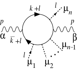
Figure 7: A QED diagram where the photons with vanishing four-momenta (denoted by dashed lines) have a given cyclic ordering $\mu_{1}\ldots\mu_{n}$. Lines $\mu_{1}$ and $\mu_{n}$ are in the proof assigned momenta $l\neq 0$.

Let $\Pi_{\mu_{1}\ldots\mu_{n}}^{\alpha\beta}(p)$ denote a quark loop correction to a photon propagator with momentum $p$ and Lorentz indices $\alpha,\beta$. The $n$ external, zero-momentum gluons attached to the quark loop have Lorentz indices $\mu_{1}\ldots\mu_{n}$, and their color indices $a_{1},\ldots,a_{n}$ are implicit. The QED result

$$\Pi_{\mu_{1}\ldots\mu_{n}}^{\alpha\beta}(p)=0\ \ {\rm for}\ \ n\geq 1$$ (85)

also holds in QCD for $n=1$ since ${\rm Tr}\,T^{a_{1}}=0$, and for $n=2$ because the color factor is then simply $\propto\delta^{a_{1}a_{2}}$. For $n\geq 3$ the QCD amplitude $\Pi_{\mu_{1}\ldots\mu_{n}}^{\alpha\beta}(p)$ differs from the QED one because the various diagrams are weighted by different color factors of the type ${\rm Tr}\left[T^{a_{1}}\ldots T^{a_{n}}\right]$. We now show that the part of the QCD amplitude which corresponds to a given color factor formally vanishes by itself. This ensures the vanishing of the complete QCD amplitude.

Consider the part of the corresponding QED amplitude which is built from all diagrams that have the same cyclic ordering of the external photon lines $\mu_{1}\ldots\mu_{n}$, where the indices are numbered by following the fermion loop against the direction of the fermion arrow. There are many diagrams of this type, which are distinguished by the positions of the two photon lines with momentum $p$ and indices $\alpha,\beta$ in the sequence of cyclically ordered external photons (see Fig. 7). We temporarily take the photons with indices $\mu_{1}$ and $\mu_{n}$ to carry incoming momenta $l$ and $-l$, respectively, while the photons $\mu_{2}\ldots\mu_{n-1}$ have vanishing four-momenta. Denoting the amplitude just described by $T_{\mu_{1}\ldots\mu_{n}}^{\alpha\beta}(p,l)$, we wish to show that $T_{\mu_{1}\ldots\mu_{n}}^{\alpha\beta}(p,0)=0$.

The momentum $l$ may be taken to flow in the direction of the fermion arrow between the vertices $\mu_{1}$ and $\mu_{n}$, and not beyond. According to (46) the derivative $-e\partial/\partial l^{\mu_{n+1}}$ applied to $T_{\mu_{1}\ldots\mu_{n}}^{\alpha\beta}(p,l)$ then generates all QED diagrams with $(n+1)$ external zero-momentum photons having the cyclic ordering $\mu_{1}\ldots\mu_{n+1}$:

$$\left.-e\frac{\partial}{\partial l^{\mu_{n+1}}}T_{\mu_{1}\ldots\mu_{n}}^{\alpha\beta}(p,l)\right|_{l=0}=T_{\mu_{1}\ldots\mu_{n}\mu_{n+1}}^{\alpha\beta}(p,l=0)$$ (86)

Assuming that the Taylor expansion

$$T_{\mu_{1}\ldots\mu_{n}}^{\alpha\beta}(p,l)=T_{\mu_{1}\ldots\mu_{n}}^{\alpha\beta}(p,0)+l^{\mu_{n+1}}\left.\frac{\partial}{\partial l^{\mu_{n+1}}}T_{\mu_{1}\ldots\mu_{n}}^{\alpha\beta}(p,l)\right|_{l=0}+{\cal O}\left(l^{2}\right)$$ (87)

is well-defined we obtain

$$T_{\mu_{1}\ldots\mu_{n}}^{\alpha\beta}(p,l)=T_{\mu_{1}\ldots\mu_{n}}^{\alpha\beta}(p,0)-\frac{1}{e}\,l^{\mu_{n+1}}T_{\mu_{1}\ldots\mu_{n}\mu_{n+1}}^{\alpha\beta}(p,0)+{\cal O}\left(l^{2}\right)$$ (88)

It is readily seen from the charge conjugation symmetry that

$$T_{\mu_{n}\ldots\mu_{1}}^{\alpha\beta}(p,l)=(-1)^{n}T_{\mu_{1}\ldots\mu_{n}}^{\alpha\beta}(p,l)$$ (89)

Reversing the order of $\mu_{1}\ldots\mu_{n}$ in (88) and recalling that the amplitudes were constructed to be cyclically symmetric in the Lorentz indices of the zero-momentum photons,

$$T_{\mu_{n}\ldots\mu_{1}\mu_{n+1}}^{\alpha\beta}(p,0)=T_{\mu_{n+1}\mu_{n}\ldots\mu_{1}}^{\alpha\beta}(p,0)$$ (90)

we get

$$(-1)^{n}T_{\mu_{1}\ldots\mu_{n}}^{\alpha\beta}(p,l)=(-1)^{n}T_{\mu_{1}\ldots\mu_{n}}^{\alpha\beta}(p,0)-\frac{1}{e}(-1)^{n+1}l^{\mu_{n+1}}T_{\mu_{1}\ldots\mu_{n}\mu_{n+1}}^{\alpha\beta}(p,0)+{\cal O}\left(l^{2}\right)$$ (91)

Comparing (88) and (91) we arrive at

$$T_{\mu_{1}\ldots\mu_{n+1}}^{\alpha\beta}(p,0)=0$$ (92)

for $n\geq 2$. Since all QCD amplitudes with the same cyclic ordering $\mu_{1}\ldots\mu_{n}$ of the external gluons have the same color factor ${\rm Tr}\left[T^{a_{1}}\ldots T^{a_{n}}\right]$ this proof for QED implies that (85) holds also in QCD.

Appendix D Quark-photon vertex $\Gamma^{\mu}(k,\bar{k})$

In this appendix we solve the implicit equation (50) for the $\gamma{\rm q}{\rm\bar{q}}\$ vertex $\Gamma^{\mu}$ in the case of the chirally invariant quark propagator (20),

$$S_{1}(p)=a_{p}\,\parbox[b]{6.00006pt}{$p$}\parbox[b]{5.50003pt}{ \raisebox{-0.86108pt}{$/$}}\ \ ;\ \ a_{p}=\frac{1}{2\mu^{2}}\left(1-\sqrt{1-\frac{4\mu^{2}}{p^{2}}}\right)$$ (93)

Using this expression for $S(p)$ (50) becomes

$$\Gamma^{\mu}(k,\bar{k})=\gamma^{\mu}-{\textstyle\frac{1}{2}}f\gamma^{\nu}\parbox[b]{6.00006pt}{$k$}\parbox[b]{5.50003pt}{ \raisebox{-0.86108pt}{$/$}}\Gamma^{\mu}(k,\bar{k})\parbox[b]{6.00006pt}{$\bar{k}$}\parbox[b]{5.50003pt}{ \raisebox{-0.86108pt}{$/$}}\gamma_{\nu}$$ (94)

where we introduced the dimensionful parameter $f$,

$$f=\mu^{2}a_{k}a_{\bar{k}}$$ (95)

Chiral and parity invariance restricts $\Gamma^{\mu}(k,\bar{k})$ to the form

$$\Gamma^{\mu}(k,\bar{k})=A_{0}\gamma^{\mu}+A_{1}k^{\mu}\parbox[b]{6.00006pt}{$k$}\parbox[b]{5.50003pt}{ \raisebox{-0.86108pt}{$/$}}+A_{2}k^{\mu}\parbox[b]{6.00006pt}{$\bar{k}$}\parbox[b]{5.50003pt}{ \raisebox{-0.86108pt}{$/$}}+A_{3}{\bar{k}}^{\mu}\parbox[b]{6.00006pt}{$k$}\parbox[b]{5.50003pt}{ \raisebox{-0.86108pt}{$/$}}+A_{4}{\bar{k}}^{\mu}\parbox[b]{6.00006pt}{$\bar{k}$}\parbox[b]{5.50003pt}{ \raisebox{-0.86108pt}{$/$}}+iA_{5}\gamma_{5}\epsilon^{\mu}(\gamma,k,\bar{k})$$ (96)

where we defined

$$\epsilon^{\mu}(\gamma,k,\bar{k})=\epsilon^{\mu\nu\rho\sigma}\gamma_{\nu}k_{\rho}{\bar{k}}_{\sigma}$$ (97)

We find the coefficients $A_{i}$ by inserting (96) into (94) and using

$$\parbox[b]{6.00006pt}{$\bar{k}$}\parbox[b]{5.50003pt}{ \raisebox{-0.86108pt}{$/$}}\gamma^{\mu}\parbox[b]{6.00006pt}{$k$}\parbox[b]{5.50003pt}{ \raisebox{-0.86108pt}{$/$}} = k^{\mu}\parbox[b]{6.00006pt}{$\bar{k}$}\parbox[b]{5.50003pt}{ \raisebox{-0.86108pt}{$/$}}+{\bar{k}}^{\mu}\parbox[b]{6.00006pt}{$k$}\parbox[b]{5.50003pt}{ \raisebox{-0.86108pt}{$/$}}-k\cdot{\bar{k}}\,\gamma^{\mu}-i\gamma_{5}\epsilon^{\mu}(\gamma,k,\bar{k})$$

$$i\gamma_{5}\parbox[b]{6.00006pt}{$\bar{k}$}\parbox[b]{5.50003pt}{ \raisebox{-0.86108pt}{$/$}}\epsilon^{\mu}(\gamma,k,\bar{k})\parbox[b]{6.00006pt}{$k$}\parbox[b]{5.50003pt}{ \raisebox{-0.86108pt}{$/$}} = -i\gamma_{5}\epsilon^{\mu}(\gamma,k,\bar{k})\,k\cdot{\bar{k}}+\gamma^{\mu}\left[k^{2}{\bar{k}}^{2}-(k\cdot{\bar{k}})^{2}\right]$$ (98)

$$-k^{\mu}\left[{\bar{k}}^{2}\parbox[b]{6.00006pt}{$k$}\parbox[b]{5.50003pt}{ \raisebox{-0.86108pt}{$/$}}-k\cdot{\bar{k}}\,\parbox[b]{6.00006pt}{$\bar{k}$}\parbox[b]{5.50003pt}{ \raisebox{-0.86108pt}{$/$}}\right]-{\bar{k}}^{\mu}\left[k^{2}\parbox[b]{6.00006pt}{${\bar{k}}$}\parbox[b]{5.50003pt}{ \raisebox{-0.86108pt}{$/$}}-k\cdot{\bar{k}}\,\parbox[b]{6.00006pt}{$k$}\parbox[b]{5.50003pt}{ \raisebox{-0.86108pt}{$/$}}\right]$$

This gives the conditions

$$A_{0} = 1-fk\cdot{\bar{k}}\,(A_{0}+k\cdot{\bar{k}}\,A_{5})+fk^{2}{\bar{k}}^{2}A_{5}$$

$$A_{1} = f{\bar{k}}^{2}(A_{2}-A_{5})$$

$$A_{2} = f(A_{0}+k\cdot{\bar{k}}\,A_{5}+k^{2}A_{1})$$

$$A_{3} = f(A_{0}+k\cdot{\bar{k}}\,A_{5}+{\bar{k}}^{2}A_{4})$$

$$A_{4} = fk^{2}(A_{3}-A_{5})$$

$$A_{5} = -f(A_{0}+k\cdot{\bar{k}}\,A_{5})$$ (99)

with solutions

$$A_{0}=\frac{1+fk\cdot{\bar{k}}}{1+2fk\cdot{\bar{k}}+f^{2}k^{2}{\bar{k}}^{2}}\ \ \ \ A_{5}=\frac{-f}{1+2fk\cdot{\bar{k}}+f^{2}k^{2}{\bar{k}}^{2}}$$ ;

$$k^{2}A_{1}={\bar{k}}^{2}A_{4}=-\frac{2fk^{2}{\bar{k}}^{2}}{1-f^{2}k^{2}{\bar{k}}^{2}}A_{5}\ \ \ \ A_{2}=A_{3}=-\frac{1+f^{2}k^{2}{\bar{k}}^{2}}{1-f^{2}k^{2}{\bar{k}}^{2}}A_{5}$$ ; (100)

The result for $\Gamma^{\mu}(k,\bar{k})$ then follows from (96):

$$\Gamma^{\mu}(k,\bar{k}) = \frac{1}{1+2fk\cdot{\bar{k}}+f^{2}k^{2}{\bar{k}}^{2}}\left\{(1+fk\cdot{\bar{k}})\gamma^{\mu}-fi\gamma_{5}\,\epsilon^{\mu\nu\rho\sigma}\gamma_{\nu}k_{\rho}{\bar{k}}_{\sigma}\phantom{\frac{f^{2}}{f^{2}}}\right.$$ (101)

$$+ \left.\frac{2f^{2}}{1-f^{2}k^{2}{\bar{k}}^{2}}(k^{\mu}\parbox[b]{6.00006pt}{$k$}\parbox[b]{5.50003pt}{ \raisebox{-0.86108pt}{$/$}}{\bar{k}}^{2}+{\bar{k}}^{\mu}\parbox[b]{6.00006pt}{$\bar{k}$}\parbox[b]{5.50003pt}{ \raisebox{-0.86108pt}{$/$}}k^{2})+\frac{f(1+f^{2}k^{2}{\bar{k}}^{2})}{1-f^{2}k^{2}{\bar{k}}^{2}}(k^{\mu}\parbox[b]{6.00006pt}{$\bar{k}$}\parbox[b]{5.50003pt}{ \raisebox{-0.86108pt}{$/$}}+{\bar{k}}^{\mu}\parbox[b]{6.00006pt}{$k$}\parbox[b]{5.50003pt}{ \raisebox{-0.86108pt}{$/$}})\right\}$$

Let us check that this expression for the vertex satisfies the Ward-Takahashi relation (52). Straightforward algebra yields:

$$p_{\mu}\Gamma^{\mu}(k,\bar{k})=\parbox[b]{6.00006pt}{$k$}\parbox[b]{5.50003pt}{ \raisebox{-0.86108pt}{$/$}}\frac{1-f{\bar{k}}^{2}}{1-f^{2}k^{2}{\bar{k}}^{2}}-\parbox[b]{6.00006pt}{$\bar{k}$}\parbox[b]{5.50003pt}{ \raisebox{-0.86108pt}{$/$}}\frac{1-fk^{2}}{1-f^{2}k^{2}{\bar{k}}^{2}}$$ (102)

Using (95) and Eq. (18) (for $b=0$),

$$a_{p}-\frac{1}{p^{2}}=\mu^{2}a_{p}^{2}$$ (103)

we get

$$\frac{1-f{\bar{k}}^{2}}{1-f^{2}k^{2}{\bar{k}}^{2}}=\frac{1}{k^{2}a_{k}}\ \ ;\ \ \frac{1-f{k}^{2}}{1-f^{2}k^{2}{\bar{k}}^{2}}=\frac{1}{\bar{k}^{2}a_{\bar{k}}}$$ (104)

Substituting these expressions in (102) gives the Ward-Takahashi relation (52).

References

-
[1]
M. A. Shifman, A. I. Vainshtein and V. I. Zakharov,
Nucl. Phys. B 147 (1979) 385, 448, 519;
E.V. Shuryak, Phys. Rept. 115 (1984) 151. -
[2]
C. D. Roberts and S. M. Schmidt, Prog. Part. Nucl. Phys. 45 (2000) S1;
R. Alkofer and L. von Smekal, Phys. Rept. 353 (2001) 281;
P. Maris and C. D. Roberts, Int. J. Mod. Phys. E 12 (2003) 297;
P. Maris and C. D. Roberts, Int. J. Mod. Phys. E 12 (2003) 297 [arXiv:nucl-th/0301049]. M. R. Pennington, arXiv:hep-ph/0409156. - [3] G. ’t Hooft, Nucl. Phys. B 72 (1974) 461; Nucl. Phys. B 75 (1974) 461.
- [4] P. Hoyer and S. Peigné, arXiv:hep-ph/0304010.
- [5] F. D. R. Bonnet, P. O. Bowman, D. B. Leinweber, A. G. Williams and J. b. Zhang [CSSM Lattice collaboration], Phys. Rev. D 65 (2002) 114503 [arXiv:hep-lat/0202003].
- [6] H. J. Munczek and A. M. Nemirovsky, Phys. Rev. D 28 (1983) 181.
- [7] X. d. Li and C. M. Shakin, arXiv:nucl-th/0409042.
- [8] F. D. R. Bonnet, P. O. Bowman, D. B. Leinweber, A. G. Williams and J. M. Zanotti, Phys. Rev. D 64 (2001) 034501 [arXiv:hep-lat/0101013].