The role of strange sea quarks in
chiral extrapolations on the lattice

Abstract

Since the strange quark has a light mass of order $O(\Lambda_{QCD})$, fluctuations of sea $s\bar{s}$ pairs may play a special role in the low-energy dynamics of QCD by inducing significantly different patterns of chiral symmetry breaking in the chiral limits $N_{f}=2$ ($m_{u}=m_{d}=0$, $m_{s}$ physical) and $N_{f}=3$ ($m_{u}=m_{d}=m_{s}=0$). This effect of vacuum fluctuations of $s\bar{s}$ pairs is related to the violation of the Zweig rule in the scalar sector, described through the two $O(p^{4})$ low-energy constants $L_{4}$ and $L_{6}$ of the three-flavour strong chiral lagrangian. In the case of significant vacuum fluctuations, three-flavour chiral expansions might exhibit a numerical competition between leading- and next-to-leading-order terms according to the chiral counting, and chiral extrapolations should be handled with a special care. We investigate the impact of the fluctuations of $s\bar{s}$ pairs on chiral extrapolations in the case of lattice simulations with three dynamical flavours in the isospin limit. Information on the size of the vacuum fluctuations can be obtained from the dependence of the masses and decay constants of pions and kaons on the light quark masses. Even in the case of large fluctuations, corrections due to the finite size of spatial dimensions can be kept under control for large enough boxes ($L\sim 2.5$ fm).

In order to achieve a better understanding of nonperturbative features of the strong interaction, it is interesting to recall the particular mass hierarchy followed by the light quarks:

$$m_{u}\sim m_{d}\ll m_{s}\sim\Lambda_{QCD}\ll\Lambda_{H}\,,$$ (1)

where $\Lambda_{QCD}$ is the characteristic scale describing the running of the QCD effective coupling and $\Lambda_{H}\sim 1$ GeV the mass scale of the bound states not protected by chiral symmetry. Therefore, the strange quark may play a special role in the low-energy dynamics of QCD:

i) it is light enough to allow for a combined expansion of observables in powers of $m_{u},m_{d},m_{s}$ around the $N_{f}=3$ chiral limit (meaning 3 massless flavours):

$$N_{f}=3:\qquad m_{u}=m_{d}=m_{s}=0\,,$$ (2)

ii) it is sufficiently heavy to induce significant changes in order parameters from the $N_{f}=3$ chiral limit to the $N_{f}=2$ chiral limit (meaning 2 massless flavours):

$$N_{f}=2:\qquad m_{u}=m_{d}=0\qquad m_{s}{\rm\ physical}\,,$$ (3)

iii) it is too light to suppress efficiently loop effects of massive $\bar{s}s$ pairs (contrary to $c,b,t$ quarks).

These three arguments suggest that $\bar{s}s$ sea-pairs may play a significant role in chiral dynamics leading to different behaviours of QCD in $N_{f}=2$ and $N_{f}=3$ chiral limits. Then, chiral order parameters such as the quark condensate and the pseudoscalar decay constant:

$$\Sigma(N_{f})=-\lim_{N_{f}}\langle\bar{u}u\rangle\,,\qquad\qquad F^{2}(N_{f})=\lim_{N_{f}}F^{2}_{\pi}\,,$$ (4)

would have significantly different values in the two chiral limits ($\lim_{N_{f}}$ denoting the chiral limit with $N_{f}$ massless flavours).

The role of $\bar{s}s$-pairs in the structure of QCD vacuum is a typical loop effect. Therefore, it should be suppressed in the large-$N_{c}$ limit, and it can be significant only if the Zweig rule is badly violated in the vacuum (scalar) channel $J^{PC}=0^{++}$. On general theoretical grounds param , one expects $\bar{s}s$ sea-pairs to have a paramagnetic effect on chiral order parameters. The latter should decrease when the strange quark mass is sent to zero : for instance, $\Sigma(2;m_{s})\geq\Sigma(2;m_{s}=0)$, and similarly for $F^{2}$. This corresponds to

$$\Sigma(2)\geq\Sigma(3)\,,\qquad F^{2}(2)\geq F^{2}(3)\,.$$ (5)

However, the size of this paramagnetic suppression is not predicted.

This effect can also be discussed in terms of the Euclidean QCD Dirac operator, more precisely of its eigenvalue spectrum (with an appropriate weight over the gluonic configurations) lssr ; stern . Chiral order parameters are related to the accumulation of the lowest eigenvalues in the thermodynamic limit. For instance, the quark condensate can be interpreted as the average density of eigenvalues around 0. In this language, the Zweig-rule violating effect due to $\bar{s}s$ pairs corresponds to multi-point correlations in the density of eigenvalues around 0 param . The size of the paramagnetic suppression eq. (5) depends on the importance of such correlations which can be interpreted as fluctuations .

Thus, it is highly desirable to extract the size of the chiral order parameters in $N_{f}=2$ and $N_{f}=3$ limits from experiment. Recent data on $\pi\pi$ scattering E865 together with older data and numerical solutions of the Roy equations ACGL allowed us to determine the two-flavour order parameters expressed in suitable physical units pipi :

$$X(2) = \frac{(m_{u}+m_{d})\Sigma(2)}{F_{\pi}^{2}M_{\pi}^{2}}=0.81\pm 0.07\,,$$ (6)

$$Z(2) = \frac{F^{2}(2)}{F_{\pi}^{2}}=0.89\pm 0.03\,.$$ (7)

A different analysis of the data in ref. E865 , with the additional input of dispersive estimates for the scalar radius of the pion, led to an even larger value of $X(2)$ CGL . In any case, $X(2)$ and $Z(2)$ are close to 1, so that corrections related to $m_{u},m_{d}\neq 0$ (while $m_{s}$ remains at its physical value) have no significant impact on the low-energy behaviour of QCD. In turn, two-flavour Chiral Perturbation Theory ($\chi$PT) chpt2 , which consists in an expansion in powers of $m_{u}$ and $m_{d}$ around the $N_{f}=2$ chiral limit, should suffer from no particular problems of convergence. Indeed, its two $O(p^{2})$ low-energy constants $F^{2}(2)$ and $\Sigma(2)$ are dominant in the expansions of the decay constant and mass of the pion.

Unfortunately, two-flavour $\chi$PT chpt2 deals only with dynamical pions in a very limited range of energy. In order to include $K$- and $\eta$-mesons dynamically and extend the energy range of interest, one must use three-flavour $\chi$PT chpt3 where the expansion in the three light quark masses starts around the $N_{f}=3$ vacuum $m_{u}=m_{d}=m_{s}=0$. From the above discussion, large vacuum fluctuations of $\bar{s}s$ pairs should have a dramatic effect on $N_{f}=3$ chiral expansions. The leading-order (LO) term, which depends on the $O(p^{2})$ low-energy constants $F^{2}(3)$ and $\Sigma(3)$, would be damped. On the other hand, next-to-leading-order (NLO) corrections could be enhanced, in particular those related to Zweig-rule violation in the scalar sector. For instance, the Gell-Mann–Oakes–Renner relation would not be saturated by its LO term and would receive sizeable numerical contributions from terms counted as NLO in the chiral counting.

We called unstability of the expansion such a numerical competition between terms of different chiral counting. A naïve argument based on resonance saturation suggests that higher orders in the chiral expansion should be suppressed by powers of $(M_{\pi}/\Lambda_{H})^{2}$. However, such an argument does not apply to a leading-order contribution proportional to $\Sigma(3)$ : there is no resonance that could saturate the quark condensate. We expect therefore to encounter three-flavour chiral expansions with a good overall convergence:

$$A=A_{LO}+A_{NLO}+A\delta A\,,\qquad\qquad\delta A\ll 1\,,$$ (8)

but the numerical balance between the leading order $A_{LO}$ and the next-to-leading order $A_{NLO}$ depends on the importance of vacuum fluctuations.

At the level of $O(p^{4})$ $N_{f}=3$ chiral perturbation theory, the size of the vacuum fluctuations is encoded in the low-energy constants (LECs) $L_{4}$ and $L_{6}$ whose values remain largely unknown. For a long time, one set them to 0 at an arbitrary hadronic scale (typically the $\eta$-mass) assuming that the Zweig rule held in the scalar sector. More recent but indirect analyses based on dispersive methods uuss ; uuss2 ; roypika suggest values of $L_{4}$ and $L_{6}$ which look quite modest but are enough to drive the three-flavour order parameters $\Sigma(3)$ and $F^{2}(3)$ down to half of their two-flavour counterparts $\Sigma(2)$ and $F^{2}(2)$. Obvioulsy, these indirect hints of sizeable vacuum fluctuations call for a more direct confirmation.

Unstable $N_{f}=3$ chiral expansions ($A_{LO}\sim A_{NLO}$) require a more careful treatment than in two-flavour $\chi$PT where such unstabilities do not occur. For instance, it would be wrong to believe that the chiral expansion of $1/A$ converges nicely . This might induce the observed problems of convergence in current two-loop computations bijnens ; bijnens2  : the latter treat the fluctuations encoded in $L_{4}$ and $L_{6}$ as small and are not designed to cope with a large violation of the Zweig rule in the scalar sector, leading to unstabilities of the chiral series.

In a previous work resum , we proposed a framework to deal with chiral expansions in the case of large fluctuations, by picking up a subset of observables with (hopefully) good convergence properties and resumming the fluctuation terms containing the Zweig-rule violating LECs $L_{4}$ and $L_{6}$. This framework includes consistently the alternatives of large and small vacuum fluctuations.

Obviously, there is a price to pay for this extension: some usual $O(p^{4})$ relations cannot be exploited anymore, because of our ignorance about their convergence. Let us comment on a few novelties in our framework:

• Observables with a good convergence, eq. (8), form a linear space, which we identify with connected QCD correlators away from kinematic singularities. This choice promotes $F_{P}^{2}$ and $F_{P}^{2}M_{P}^{2}$ ($P=\pi,K,\eta$) : LO and NLO may compete, but there should be only a tiny contribution form NNLO and higher. On the contrary, the chiral expansion of $M_{P}^{2}$ (ratio of the former quantities) may exhibit a bad convergence.

  In principle, two-loop computations could provide a check of these assumptions. However, it is difficult to exploit available analyses bijnens ; bijnens2 for two reasons: i) in the algebraic expressions, low-energy constants are traded for physical quantities assuming that the chiral expansions of the latter are dominated numerically by the LO contribution, ii) the numerical results rely on a specific model of resonance saturation for the $O(p^{6})$ LECs . The dependence on these two assumptions should be assessed before any definite conclusion can be drawn from two-loop computations . Obviously, if eq. (8) were not followed by $F_{P}^{2}$ and $F_{P}^{2}M_{P}^{2}$, but rather by other combinations of $F_{P}$ and $M_{P}$, some of our conclusions might be modified, but this task is beyond the scope of the present paper.

• The three-flavour quark condensate and pseudoscalar decay constant expressed in physical units:

  $$X(3)=\frac{2m\Sigma(3)}{F_{\pi}^{2}M_{\pi}^{2}}\,,\qquad\qquad Z(3)=\frac{F^{2}(3)}{F_{\pi}^{2}}\,,$$ (9)

  are free parameters. Constraints come from the vacuum stability and the paramagnetic inequalities (5):

  $$0\leq X(3)\leq X(2)\,,\qquad\qquad 0<Z(3)\leq Z(2)\,,$$ (10)

  where the values of $X(2)$ and $Z(2)$ have been determined from experiment, see eqs. (6-(7).

• The quark mass ratio $r=m_{s}/m$ ($m=m_{u}=m_{d}$) cannot be fixed from $M_{K}^{2}/M_{\pi}^{2}$ since we do not control the convergence of its three-flavour chiral expansion. $r$ becomes a free parameter which can vary in the range:

  $$r_{1}=2\frac{F_{K}M_{K}}{F_{\pi}M_{\pi}}-1\sim 8\leq r\leq r_{2}=2\frac{F_{K}^{2}M_{K}^{2}}{F_{\pi}^{2}M_{\pi}^{2}}-1\sim 36\,.$$ (11)

  The chiral expansions of $F_{\pi}^{2}M_{\pi}^{2}$ and $F_{K}^{2}M_{K}^{2}$ lead to a correlation between $r$ and $X(2)$ param . Experimentally, the analysis of $\pi\pi$ scattering phase shifts E865 shows that $r>14$ (95% CL), slightly favouring values between 20 and 25 resum .

• The agreement of the pseudoscalar spectrum with the Gell-Mann–Okubo formula requires a fine tuning of $L_{7}$. Let us remark though that this fine tuning exists even in the case of a dominant three-flavour quark condensate and small vacuum fluctuations resum .

• One cannot determine LECs or combinations of LECs through ratios of observables. For instance, one should not use $F_{K}/F_{\pi}$ to determine $L_{5}$ because we do not know if the chiral expansion of $F_{K}/F_{\pi}$ converges at all.

There are some prospects of probing experimentally the three-flavour sector and in particular the size of vacuum fluctuations through $\pi K$ scattering roypika . Unfortunately, the current data are not precise enough to draw any definite conclusion. On the other hand, recent progress achieved by lattice unquenched simulations lattrev makes them an interesting field to investigate the size of vacuum fluctuations. For instance, lattice practitionners can vary very easily the value of the quark masses.

A comment is in order at this point. From large-$N_{c}$ considerations, it is often assumed that quark-loop effects are not significant, so that simulations with only two dynamical flavours, or even none (quenched case), could be good approximations to real QCD. We are precisely questionning this assumption in the case of observables related to chiral symmetry breaking. Thus, it is mandatory to perform unquenched simulations with three dynamical flavours in order to probe strange sea-quark effects on the pattern of chiral symmetry breaking,

One could think of investigating directly the correlations of Dirac eigenvalues, or the $m_{s}$-dependence of the quark condensate and pseudoscalar decay constant. However, this might prove rather challenging tasks since they require simulations with three dynamical very light quarks. In this paper, we investigate another way of probing the size of vacuum fluctuations through the spectrum of the theory. Indeed, this less immediate approach is easier to follow with current lattice simulations. We believe that this exercise might also be useful to illustrate some subtleties arising in three-flavour chiral extrapolations when vacuum fluctuations of $s\bar{s}$ pairs are not negligible.

We are not going to address the issue of discretisation, which depends on the specific implementation of the lattice action. We focus on chiral extrapolations with potentially large vacuum fluctuations and on the impact of finite-volume corrections. For definiteness, we work in the isospin limit $m_{u}=m_{d}=m$ and we consider a lattice simulation with (2+1) flavours : two flavours are set to a common mass $\tilde{m}$, whereas the third one is kept at the same mass as the physical strange quark $m_{s}$. Each quantity $X$ observed in the physical situation $(m,m,m_{s})$ has a lattice counterpart $\tilde{X}$ for $(\tilde{m},\tilde{m},m_{s})$.

We introduce the notation:

$$q=\frac{\tilde{m}}{m_{s}}\,, r=\frac{m_{s}}{m}\,,$$ (12)

$$X(3)=\frac{2m\Sigma(3)}{F_{\pi}^{2}M_{\pi}^{2}}\,, Z(3)=\frac{F^{2}(3)}{F_{\pi}^{2}}\,,$$ (13)

$$Y(3) = \frac{X(3)}{Z(3)}=\frac{2mB_{0}}{M_{\pi}^{2}}\,,$$ (14)

where $\Sigma(3)$ and $F(3)$ are (the absolute value of) the quark condensate and the pion decay constant in the $N_{f}=3$ chiral limit, and $B_{0}=\Sigma(3)/F(3)^{2}$. We take the following values for the masses and decay constants: $F_{\pi}=92.4$ MeV, $F_{K}/F_{\pi}=1.22$, $M_{\pi}=139.6$ MeV, $M_{K}=493.7$ MeV, $M_{\eta}=547$ MeV.

1 Vacuum fluctuations at infinite volume

1.1 Bare expansions of masses and decay constants

We start by considering the impact of vacuum fluctuations on the spectrum in the limit $L\to\infty$. Since large vacuum fluctuations are allowed, the problems highlighted in the introduction might arise. Therefore, we have to define the appropriate observables to consider and the treatment of their chiral expansion. We follow the procedure advocated in resum , reexpressing it in an equivalent way convenient for our purposes:

1. Consider a subset of observables that are assumed to have a good overall convergence – we call them “good observables”. They must form a linear space, which we choose to be that of connected QCD correlators (of vector/axial currents and their divergences) as functions of external momenta, away from any kinematic singularities. This rule selects in particular $F_{P}^{2}$ and $F_{P}^{2}M_{P}^{2}$.

2. Take each observable and write its NLO chiral expansion.

3. In theses formulae, reexpand the physical quantities (masses, decay constants…) in powers of quark masses wherever the resulting dependence on the latter is polynomial. Keep the physical quantities only in the nonanalytic terms (unitarity cuts, logarithmic divergences…). The result is called “bare expansion”.

4. In the bare expansions, reexpress $O(p^{2})$ and $O(p^{4})$ LECs in terms of $X(3)$, $Z(3)$ and $r$ using exact Ward identities for pseudoscalar masses and decay constants.

The first step is straightforward : one has to compute the NLO chiral expansion of the masses and decay constants of Goldstone bosons in an infinite volume with the quark masses $m_{u}=m_{d}=\tilde{m}$ and $m_{s}$. The expressions can be obtained directly from ref. chpt3 . Then, we must reexpand the physical quantities occuring in these formulae in terms of the quark masses wherever the dependence is analytic. In the case of $\tilde{F}_{P}^{2}$ and $\tilde{F}_{P}^{2}\tilde{M}_{P}^{2}$, the only issue lies in tadpole contributions such as:

$$\frac{\tilde{M}_{\pi}^{2}}{16\pi^{2}}\log\frac{\tilde{M}_{\pi}^{2}}{\mu^{2}}\,.$$ (15)

To obtain the bare expansions associated with $\tilde{F}_{P}^{2}$ and $\tilde{F}_{P}^{2}\tilde{M}_{P}^{2}$, we keep the physical masses only in the (nonanalytic) logarithm but we expand the front factor in powers of quark masses. Hence, at the chiral order we are working, the contribution from the pion tadpole has the following bare expansion:

$$\frac{2{\tilde{m}}B_{0}}{16\pi^{2}}\log\frac{{\tilde{M}}_{\pi}^{2}}{\mu^{2}}\,.$$ (16)

In the bare expansion, the polynomial structure in the quark masses is explictly displayed, so that we can keep track of the relative contribution of the LO, NLO, NNLO$\ldots$ terms.

The resulting bare expansions for the decay constants (third step of our procedure) can be expressed in the following way:

$$\frac{\tilde{F}_{\pi}^{2}}{F_{\pi}^{2}}=Z(3)+\frac{M_{\pi}^{2}}{F_{\pi}^{2}}qrY(3)\left[8\left(\frac{1}{q}+2\right)L_{4}^{r}+8L_{5}^{r}\right]$$ (17)

$$\qquad-\frac{M_{\pi}^{2}}{F_{\pi}^{2}}\frac{1}{32\pi^{2}}qrY(3)\left[4\log\frac{\tilde{M}_{\pi}^{2}}{\mu^{2}}+\left(\frac{1}{q}+1\right)\log\frac{\tilde{M}_{K}^{2}}{\mu^{2}}\right]$$

$$\qquad+\frac{\tilde{F}_{\pi}^{2}}{F_{\pi}^{2}}\tilde{e}_{\pi}\,,$$

$$\frac{\tilde{F}_{K}^{2}}{F_{\pi}^{2}}=Z(3)$$ (18)

$$\qquad+\frac{M_{\pi}^{2}}{F_{\pi}^{2}}qrY(3)\left[8\left(\frac{1}{q}+2\right)L_{4}^{r}+4\left(\frac{1}{q}+1\right)L_{5}^{r}\right]$$

$$\qquad-\frac{M_{\pi}^{2}}{F_{\pi}^{2}}\frac{1}{32\pi^{2}}qrY(3)\Bigg{[}\frac{3}{2}\log\frac{\tilde{M}_{\pi}^{2}}{\mu^{2}}$$

$$\qquad\qquad+\frac{3}{2}\left(\frac{1}{q}+1\right)\log\frac{\tilde{M}_{K}^{2}}{\mu^{2}}+\frac{1}{2}\left(\frac{2}{q}+1\right)\log\frac{\tilde{M}_{\eta}^{2}}{\mu^{2}}\Bigg{]}$$

$$\qquad+\frac{\tilde{F}_{K}^{2}}{F_{\pi}^{2}}\tilde{e}_{K}\,,$$

$$\frac{\tilde{F}_{\eta}^{2}}{F_{\pi}^{2}}=Z(3)]$$ (19)

$$\qquad+\frac{M_{\pi}^{2}}{F_{\pi}^{2}}qrY(3)\left[8\left(\frac{1}{q}+2\right)L_{4}^{r}+\frac{8}{3}\left(\frac{2}{q}+1\right)L_{5}^{r}\right]$$

$$\qquad-\frac{M_{\pi}^{2}}{F_{\pi}^{2}}\frac{1}{32\pi^{2}}qrY(3)\times 3\left(\frac{1}{q}+1\right)\log\frac{\tilde{M}_{K}^{2}}{\mu^{2}}+\frac{\tilde{F}_{\eta}^{2}}{F_{\pi}^{2}}\tilde{e}_{\eta}\,,$$

where $\tilde{e}_{P}$ are NNLO remainders of $O(m_{q}^{2})$ ($m_{q}$ denotes either $m_{s}$ or $\tilde{m}$). We have divided by the physical value of $F_{\pi}^{2}$ in order to deal with dimensionless quantities.

In a similar way, we obtain the bare expansions of the masses:

$$\frac{\tilde{F}_{\pi}^{2}\tilde{M}_{\pi}^{2}}{F_{\pi}^{2}M_{\pi}^{2}}=qr\Bigg{\{}X(3)$$

$$\qquad+\frac{M_{\pi}^{2}}{F_{\pi}^{2}}qr[Y(3)]^{2}\left[16\left(\frac{1}{q}+2\right)L_{6}^{r}+16L_{8}^{r}\right]$$

$$\qquad-\frac{M_{\pi}^{2}}{F_{\pi}^{2}}\frac{1}{32\pi^{2}}qr[Y(3)]^{2}\Bigg{[}3\log\frac{\tilde{M}_{\pi}^{2}}{\mu^{2}}$$

$$\qquad\qquad\qquad+\left(\frac{1}{q}+1\right)\log\frac{\tilde{M}_{K}^{2}}{\mu^{2}}+\frac{1}{9}\left(\frac{2}{q}+1\right)\log\frac{\tilde{M}_{\eta}^{2}}{\mu^{2}}\Bigg{]}\Bigg{\}}$$

$$\qquad+\frac{\tilde{F}_{\pi}^{2}\tilde{M}_{\pi}^{2}}{F_{\pi}^{2}M_{\pi}^{2}}\tilde{d}_{\pi}\,,$$

$$\frac{\tilde{F}_{K}^{2}\tilde{M}_{K}^{2}}{F_{\pi}^{2}M_{\pi}^{2}}=\frac{qr}{2}\left(\frac{1}{q}+1\right)\Bigg{\{}X(3)$$

$$\qquad+\frac{M_{\pi}^{2}}{F_{\pi}^{2}}qr[Y(3)]^{2}\left[16\left(\frac{1}{q}+2\right)L_{6}^{r}+8\left(\frac{1}{q}+1\right)L_{8}^{r}\right]$$

$$\qquad-\frac{M_{\pi}^{2}}{F_{\pi}^{2}}\frac{1}{32\pi^{2}}qr[Y(3)]^{2}\Bigg{[}\frac{3}{2}\log\frac{\tilde{M}_{\pi}^{2}}{\mu^{2}}$$

$$\qquad\qquad+\frac{3}{2}\left(\frac{1}{q}+1\right)\log\frac{\tilde{M}_{K}^{2}}{\mu^{2}}+\frac{5}{18}\left(\frac{2}{q}+1\right)\log\frac{\tilde{M}_{\eta}^{2}}{\mu^{2}}\Bigg{]}\Bigg{\}}$$

$$\qquad+\frac{\tilde{F}_{K}^{2}\tilde{M}_{K}^{2}}{F_{\pi}^{2}M_{\pi}^{2}}\tilde{d}_{K}\,,$$

$$\frac{\tilde{F}_{\eta}^{2}\tilde{M}_{\eta}^{2}}{F_{\pi}^{2}M_{\pi}^{2}}=qr\Bigg{\{}\frac{1}{3}\left(\frac{2}{q}+1\right)$$

$$\qquad\times\Bigg{(}X(3)+\frac{M_{\pi}^{2}}{F_{\pi}^{2}}qr[Y(3)]^{2}$$

$$\qquad\qquad\qquad\times\left[16\left(\frac{1}{q}+2\right)L_{6}^{r}+\frac{16}{3}\left(\frac{2}{q}+1\right)L_{8}^{r}\right]$$

$$\qquad\qquad-\frac{M_{\pi}^{2}}{F_{\pi}^{2}}\frac{1}{32\pi^{2}}qr[Y(3)]^{2}$$

$$\qquad\qquad\times\left[2\left(\frac{1}{q}+1\right)\log\frac{\tilde{M}_{K}^{2}}{\mu^{2}}+\frac{4}{9}\left(\frac{2}{q}+1\right)\log\frac{\tilde{M}_{\eta}^{2}}{\mu^{2}}\right]\Bigg{)}$$

$$\quad-\frac{M_{\pi}^{2}}{F_{\pi}^{2}}\frac{1}{32\pi^{2}}qr[Y(3)]^{2}\Bigg{[}\log\frac{\tilde{M}_{\pi}^{2}}{\mu^{2}}$$

$$\qquad\qquad-\frac{1}{3}\left(\frac{1}{q}+1\right)\log\frac{\tilde{M}_{K}^{2}}{\mu^{2}}-\frac{1}{9}\left(\frac{2}{q}+1\right)\log\frac{\tilde{M}_{\eta}^{2}}{\mu^{2}}\Bigg{]}$$

$$\quad+\frac{32}{9}\left(\frac{1}{q}-1\right)^{2}\frac{M_{\pi}^{2}}{F_{\pi}^{2}}qr[Y(3)]^{2}[3L_{7}+L_{8}^{r}]\Bigg{\}}+\frac{\tilde{F}_{\eta}^{2}\tilde{M}_{\eta}^{2}}{F_{\pi}^{2}M_{\pi}^{2}}\tilde{d}_{\eta}\,,$$

where $\tilde{d}_{P}$ are NNLO remainders of $O(m_{q}^{2})$. We have divided by the physical value of $F_{\pi}^{2}M_{\pi}^{2}$ in order to deal with dimensionless quantities.

1.2 Expression of $O(p^{4})$ LECs

We must know perform the fourth step of our procedure. As shown in refs. param ; uuss ; uuss2 ; resum , one can reexpress the $O(p^{4})$ LECs $L_{4},L_{5},L_{6},L_{8}$ in terms of $[r,X(3),Z(3)]$ (and NNLO remainders) using the four chiral expansions of $F_{P}^{2}$ and $F_{P}^{2}M_{P}^{2}$ ($P=\pi,K$) in the physical case. These quantities, related to two-point functions of axial/vector currents and of their divergences at vanishing momentum transfer, are expected to have small NNLO remainders. One obtains resum :

$$Y(3)\Delta L_{4} = \frac{1}{8(r+2)}\frac{F_{\pi}^{2}}{M_{\pi}^{2}}[1-\eta(r)-Z(3)-e]\,,$$ (23)

$$Y(3)\Delta L_{5} = \frac{1}{8}\frac{F_{\pi}^{2}}{M_{\pi}^{2}}[\eta(r)+e^{\prime}]\,,$$ (24)

$$Y^{2}(3)\Delta L_{6} = \frac{1}{16(r+2)}\frac{F_{\pi}^{2}}{M_{\pi}^{2}}[1-\epsilon(r)-X(3)-d]\,,$$ (25)

$$Y^{2}(3)\Delta L_{8} = \frac{1}{16}\frac{F_{\pi}^{2}}{M_{\pi}^{2}}[\epsilon(r)+d^{\prime}]\,.$$ (26)

$\Delta L_{i}=L_{i}^{r}(\mu)-\hat{L}_{i}(\mu)$ combine the (renormalized and quark-mass independent) constants $L_{4,5,6,8}$ and chiral logarithms so that they are independent of the renormalisation scale $\mu$:

$$32\pi^{2}\hat{L}_{4}(\mu) = \frac{1}{8}\log\frac{M_{K}^{2}}{\mu^{2}}-\frac{1}{8(r-1)(r+2)}$$

$$\times\left[(4r+1)\log\frac{M_{K}^{2}}{M_{\pi}^{2}}+(2r+1)\log\frac{M_{\eta}^{2}}{M_{K}^{2}}\right]\,,$$

$$32\pi^{2}\hat{L}_{5}(\mu) = \frac{1}{8}\left[\log\frac{M_{K}^{2}}{\mu^{2}}+2\log\frac{M_{\eta}^{2}}{\mu^{2}}\right]$$

$$\quad+\frac{1}{8(r-1)}\left[3\log\frac{M_{\eta}^{2}}{M_{K}^{2}}+5\log\frac{M_{K}^{2}}{M_{\pi}^{2}}\right]\,,$$

$$32\pi^{2}\hat{L}_{6}(\mu) = \frac{1}{16}\left[\log\frac{M_{K}^{2}}{\mu^{2}}+\frac{2}{9}\log\frac{M_{\eta}^{2}}{\mu^{2}}\right]$$

$$-\frac{1}{16}\frac{r}{(r+2)(r-1)}\left[3\log\frac{M_{K}^{2}}{M_{\pi}^{2}}+\log\frac{M_{\eta}^{2}}{M_{K}^{2}}\right]\,,$$

$$32\pi^{2}\hat{L}_{8}(\mu) = \frac{1}{16}\left[\log\frac{M_{K}^{2}}{\mu^{2}}+\frac{2}{3}\log\frac{M_{\eta}^{2}}{\mu^{2}}\right]$$

$$+\frac{1}{16(r-1)}\left[3\log\frac{M_{K}^{2}}{M_{\pi}^{2}}+\log\frac{M_{\eta}^{2}}{M_{K}^{2}}\right]\,.$$

The right hand-side of eqs. (23)-(26) involves the $r$-dependent functions:

$$\epsilon(r) = 2\frac{r_{2}-r}{r^{2}-1},\quad r_{2}=2\left(\frac{F_{K}M_{K}}{F_{\pi}M_{\pi}}\right)^{2}-1\sim 36\,,$$ (31)

$$\eta(r) = \frac{2}{r-1}\left(\frac{F_{K}^{2}}{F_{\pi}^{2}}-1\right)\,,$$ (32)

whereas $d,d^{\prime}$ and $e,e^{\prime}$ are combinations of NNLO remainders associated with the chiral expansions of $\pi,K$ masses and decay constants respectively. These remainders should be small, and we are going to neglect them for all numerical estimates in the following.

We stress that eqs. (23)-(26) are nothing more than a convenient reexpression of the $N_{f}=3$ chiral expansions of $F_{\pi}^{2},F_{K}^{2},F_{\pi}^{2}M_{\pi}^{2},F_{K}^{2}M_{K}^{2}$. The latter can be easily recovered through linear combinations of eqs. (23)-(26). For instance, the chiral expansion of $F_{\pi}^{2}$ [$F_{\pi}^{2}M_{\pi}^{2}$] is obtained when one combines eqs. (23)-(24) [eqs. (25)-(26)] to eliminate $\eta(r)$ [$\epsilon(r)$].

1.3 Numerical results

To exploit the previous formulae, we have to fix the values of $r,X(3),Z(3)$. Since these parameters are only weakly constrained by experimental data, we will vary them in the ranges $r=20,30$, $Z(3)=0.4,0.8$ and $X(3)=0.2,0.4,0.8$. In each “physical” situation, we study how the masses and decay constants of the simulated $\pi$ and $K$ vary with $q$, neglecting all NNLO remainders for the moment.

A slight computational difficulty arises: in eqs. (17)-(1.1), the logarithmic NLO corrections involve the values of the simulated masses $\tilde{M}_{P}^{2}$. We could solve iteratively the system of equations to determine these masses. However, two iterations turn out to achieve a sufficient numerical accuracy. This corresponds to an easier procedure: i) compute $\hat{M}_{P}^{2}$ defined from eqs. (17)-(1.1) with $\tilde{M}_{P}^{2}$ replaced by $M_{P}^{2}$ on their right-hand side, ii) consider eqs. (17)-(1.1) again, with $\tilde{M}_{P}^{2}$ replaced by $\hat{M}_{P}^{2}$ on their right-hand side, iii) the resulting values for the pseudoscalar masses are equal to $\tilde{M}_{P}^{2}$ up to a tiny error.

In figs. 1 and 2 we have plotted $\tilde{F}_{P}^{2}$, $\tilde{F}_{P}^{2}\tilde{M}_{P}^{2}$ and $\tilde{M}_{P}^{2}$ ($P=\pi,K$) as functions of $q=\tilde{m}/m_{s}$ in an infinite volume, neglecting all NNLO remainders. For each observable, the first column corresponds to $Z(3)=0.8$, the second one to $Z(3)=0.4$. On each plot, the curves correspond to different values of $X(3)$ [full: 0.8, long-dashed: 0.4, dashed: 0.2] and of $r$ [thick: $r=30$, thin: $r=20$].

Figure 1: $\tilde{F}_{\pi}^{2}$, $\tilde{F}_{\pi}^{2}\tilde{M}_{\pi}^{2}$ and $\tilde{M}_{\pi}^{2}$ (respectively upper, middle and lower plots) normalized to their physical values as functions of $q=\tilde{m}/m_{s}$. The first (second) column corresponds to $Z(3)=0.8$ (0.4). On each plot, full, long-dashed and dashed curves correspond respectively to $X(3)=0.8,0.4,0.2$. Thick (thin) lines are drawn for $r=30$ (20). All NNLO remainders are neglected.

Figure 2: $\tilde{F}_{K}^{2}$, $\tilde{F}_{K}^{2}\tilde{M}_{K}^{2}$ and $\tilde{M}_{K}^{2}$ (respectively upper, middle and lower plots) normalised to their physical values as functions of $q=\tilde{m}/m_{s}$. The first (second) column corresponds to $Z(3)=0.8$ (0.4). On each plot, full, long-dashed and dashed curves correspond respectively to $X(3)=0.8,0.4,0.2$. Thick (thin) lines are drawn for $r=30$ (20). All NNLO remainders are neglected.

A few comments are in order:

• Our choice of normalisation imposes that all the curves intersect at the physical point $\tilde{m}=m$ where:

  $$q=\frac{1}{r}\,,\qquad\qquad\frac{\tilde{X}}{X}=1\,.$$ (33)

• If $Y(3)>1$, vacuum instability may occur : the pion mass becomes negative for “large” masses [$q=O(1)$]. This situation would occur if vacuum fluctuations had a more significant impact on the decay constant than on the condensate : the first would decrease more quickly than the latter from the physical case to the three-flavour chiral limit.

  Actually, this situation seems unlikely. A nonvanishing $F^{2}$ is equivalent to the spontaneous breakdown of chiral symmetry. Other chiral order parameters (like $\Sigma$) may or may not vanish depending on the breaking pattern. We expect therefore $F^{2}$ to be the last chiral order parameter to vanish, after or together with all the other parameters (e.g., $\Sigma$), and thus $Y(3)\leq 1$. The analysis of some properties of the small Dirac eigenvalues suggests the same conclusion lssr ; stern .

  Even though this theoretical expectation has not been checked experimentally yet, we dismiss the case $Y(3)\geq 1$ (unphysical in our opinion) in the remainder of this article.

• On the plots, very small values of $X(3)$ do not necessarily correspond to almost vanishing pion masses. Indeed, we take into acount at least two different sources of chiral symmetry breaking : quark condensation $\Sigma(3)$ and vacuum fluctuations $L_{4}$, $L_{6}$. For $X(3)=0$, chiral symmetry breaking may still be triggered by the fluctuations encoded in $L_{6}$, and the simulated pion mass may remain rather massive for $\tilde{m}\neq 0$ .

• The pseudoscalar masses $M_{P}^{2}$ are not the best candidates to observe a curvature due to chiral logarithms. The $\tilde{m}$-dependence is hardly different from a polynomial one. In addition, $X(3)$ must be much smaller than 1 to observe a variation in the curvature.

2 Finite-volume effects

2.1 NLO chiral expansions

The lattice simulations are performed in a finite spatial box, whereas time is sent to infinity to single out the ground state. For sufficiently large boxes ($L\gg 1/\Lambda_{H}$), the Goldstone modes remain the only relevant degrees of freedom, whose interactions can be described through a low-energy effective theory GLfinvol . In the case of periodic boundary conditions, this effective theory is identical to $\chi$PT, with the same values of the LECs as in an infinite volume. In addition, if the box size is large enough compared to the inverse Compton length of the pion GLfinvol ; luscher ; finvol , the so-called $p$-expansion is valid and the only difference from the infinite-volume case shows up in the propagators of the Goldstone modes. This affects only the tadpole logarithms in the formulae of the previous section:

$$\frac{\tilde{M}_{P}^{2}}{16\pi^{2}}\log\frac{\tilde{M}_{P}^{2}}{\mu^{2}}\qquad\to\qquad\frac{1}{2L^{3}}\sum_{\vec{\ell}}\frac{1}{\omega_{P}}\,,$$ (34)

where:

$$\vec{\ell}\in\frac{2\pi}{L}\times Z^{3}\,,\qquad\qquad\omega_{P}=\sqrt{\vec{\ell}^{2}+\tilde{M}_{P}^{2}}\,.$$ (35)

We obtain for the decay constants:

$$\frac{\tilde{F}_{\pi}^{2}}{F_{\pi}^{2}}=Z(3)+\frac{M_{\pi}^{2}}{F_{\pi}^{2}}qrY(3)\left[8\left(\frac{1}{q}+2\right)L_{4}^{r}+8L_{5}^{r}\right]$$ (36)

$$\qquad-\frac{1}{4F_{\pi}^{2}L^{3}}\left[4\tilde{\sigma}_{\pi}+2\tilde{\sigma}_{K}\right]\,,$$

$$\frac{\tilde{F}_{K}^{2}}{F_{\pi}^{2}}=Z(3)$$ (37)

$$\qquad+\frac{M_{\pi}^{2}}{F_{\pi}^{2}}qrY(3)\left[8\left(\frac{1}{q}+2\right)L_{4}^{r}+4\left(\frac{1}{q}+1\right)L_{5}^{r}\right]$$

$$\qquad-\frac{1}{4F_{\pi}^{2}L^{3}}\left[\frac{3}{2}\tilde{\sigma}_{\pi}+3\tilde{\sigma}_{K}+\frac{3}{2}\tilde{\sigma}_{\eta}\right]\,,$$

where:

$$\tilde{\sigma}_{P}=\sum_{\vec{\ell}}\frac{1}{\sqrt{\vec{\ell}^{2}+\tilde{M}_{P}^{2}}}\,.$$ (38)

In a similar way, we obtain for the masses:

$$\frac{\tilde{F}_{\pi}^{2}\tilde{M}_{\pi}^{2}}{F_{\pi}^{2}M_{\pi}^{2}}=qr\Bigg{\{}X(3)$$ (39)

$$\qquad+\frac{M_{\pi}^{2}}{F_{\pi}^{2}}qr[Y(3)]^{2}\left[16\left(\frac{1}{q}+2\right)L_{6}^{r}+16L_{8}^{r}\right]$$

$$\qquad-\frac{Y(3)}{4F_{\pi}^{2}L^{3}}\left[3\tilde{\sigma}_{\pi}+2\tilde{\sigma}_{K}+\frac{1}{3}\tilde{\sigma}_{\eta}\right]\Bigg{\}}\,,$$

$$\frac{\tilde{F}_{K}^{2}\tilde{M}_{K}^{2}}{F_{\pi}^{2}M_{\pi}^{2}}=\frac{qr}{2}\left(\frac{1}{q}+1\right)\Bigg{\{}X(3)$$ (40)

$$\qquad+\frac{M_{\pi}^{2}}{F_{\pi}^{2}}qr[Y(3)]^{2}\left[16\left(\frac{1}{q}+2\right)L_{6}^{r}+8\left(\frac{1}{q}+1\right)L_{8}^{r}\right]$$

$$\qquad-\frac{Y(3)}{4F_{\pi}^{2}L^{3}}\left[\frac{3}{2}\tilde{\sigma}_{\pi}+3\tilde{\sigma}_{K}+\frac{5}{6}\tilde{\sigma}_{\eta}\right]\Bigg{\}}\,.$$

2.2 Bare expansions at finite volume

The above NLO chiral expansions are not bare expansions yet. We must reexpand the physical masses in powers of quark masses wherever the dependence on the latter is polynomial. Therefore, we have to identify the nonanalytic pieces in the tadpole term $\tilde{\sigma}$, which are a logarithm due to ultraviolet divergences and a pole due to infrared divergences.

Since the (finite-volume) tadpole sum and the (infinite-volume) integral share the same ultraviolet divergences, it is convenient to introduce their difference hasenleut :

$$\xi_{s}(L,M^{2})=\frac{1}{L^{3}}\sum_{\vec{\ell}}\frac{1}{(\vec{\ell}^{2}+M^{2})^{s}}$$ (41)

$$\qquad-\frac{\sqrt{4\pi}\Gamma(s+1/2)}{\Gamma(s)}\int\frac{d^{4}q_{E}}{(2\pi)^{4}}\frac{1}{(q_{E}^{2}+M^{2})^{s+1/2}}\,.$$

$\xi$ can be evaluated as an integral of known mathematical functions finvol :

$$\xi_{s}(L,M^{2}) = \frac{1}{(4\pi)^{3/2}\Gamma(s)}$$

$$\qquad\times\int_{0}^{\infty}d\tau\tau^{s-5/2}e^{-\tau M^{2}}\left[\theta^{3}\left(\frac{L^{3}}{4\tau}\right)-1\right]\,.$$

In order to turn the previous NLO chiral expansions into bare expansions, we can isolate the nonanalytic pieces in $\tilde{\sigma}_{P}$ and expand the rest in powers of quark masses:

$$\frac{\tilde{\sigma}_{P}}{L^{3}} = \frac{\tilde{M}_{P}^{2}}{8\pi^{2}}\log\frac{\tilde{M}_{P}^{2}}{\mu^{2}}+\xi_{1/2}(L,\tilde{M}_{P}^{2})$$ (43)

$$\to \frac{{\rm LO}(\tilde{M}_{P}^{2})}{8\pi^{2}}\log\frac{\tilde{M}_{P}^{2}}{\mu^{2}}+\frac{1}{L^{3}\tilde{M}_{P}}$$

$$\qquad+\frac{{\rm LO}(\tilde{M}_{P}^{2})}{8\pi^{2}}\log\frac{{\rm LO}(\tilde{M}_{P}^{2})}{\tilde{M}_{P}^{2}}$$

$$+\Bigg{[}\xi_{1/2}(L,{\rm LO}(\tilde{M}_{P}^{2}))-\frac{1}{L^{3}\sqrt{{\rm LO}(\tilde{M}_{P}^{2})}}\Bigg{]}\,,$$

where ${\rm LO}[M_{P}^{2}]$ denotes the leading-order contribution to the meson mass:

$${\rm LO}[\tilde{M}_{\pi}^{2}] = qrY(3)M_{\pi}^{2}\,,$$ (45)

$${\rm LO}[\tilde{M}_{K}^{2}] = \frac{(q+1)r}{2}Y(3)M_{\pi}^{2}\,,$$ (46)

$${\rm LO}[\tilde{M}_{\eta}^{2}] = \frac{(q+2)r}{3}Y(3)M_{\pi}^{2}\,.$$ (47)

In App. A, we check that all the nonanalytic dependence on $\tilde{M}_{P}^{2}$ in $\tilde{\sigma}_{P}$ comes from the first two terms in eq. (2.2), whereas the last (bracketed) is analytic in ${\rm LO}(\tilde{M}_{P}^{2})$. We could take eq. (2.2) as the bare expansion of $\tilde{\sigma}_{P}$. However, a further simplification can be performed : the (last) logarithmic term in Eq. (2.2) is small whatever the size of the fluctuations and contributes to $\tilde{\sigma}_{P}$ only at NLO. We choose to absorb these terms in the NNLO remainders of the masses and decay constants and to define the bare expansion of $\tilde{\sigma}_{P}$ through:

$$\frac{\tilde{\sigma}_{P}}{L^{3}} = \frac{{\rm LO}(\tilde{M}_{P}^{2})}{8\pi^{2}}\log\frac{\tilde{M}_{P}^{2}}{\mu^{2}}+\frac{1}{L^{3}\tilde{M}_{P}}$$

$$\qquad+\left[\xi_{1/2}(L,{\rm LO}(\tilde{M}_{P}^{2}))-\frac{1}{L^{3}\sqrt{{\rm LO}(\tilde{M}_{P}^{2})}}\right]+\ldots$$

where the ellipsis denotes $O(p^{4})$ terms that are absorbed in the NNLO remainders.

First, let us notice that we recover the results of the previous section in the large-volume limit: only the first term in eq. (2.2) survives, which is exactly the bare expansion of the infinite-volume tadpoles discussed in Sec. 1.1. In addition, this choice for the bare expansion settles related issues concerning the convergence of the expansion at finite volume. $\chi$PT in a finite box can be consistently formulated in three different regimes, called $p$-, $\epsilon$- and $\delta$-expansions, depending on the relative sizes of the box sides and the pion mass GLfinvol . In particular, the $p$-expansion used here holds if:

$$F_{\pi}L\gg 1\,,\qquad\qquad M_{\pi}L\gg 1\,.$$ (49)

If the second condition is violated, the pion is too large to be contained in the box : the breakdown of the $p$-expansion is flagged by infrared divergences. In the case of small fluctuations, quark condensation is responsible for $N_{f}=3$ chiral symmetry breaking. The second condition in eq. (49) is translated into $2mB_{0}L^{2}={\rm LO}(M_{\pi}^{2})\times L^{2}\gg 1$. If either $m$ or $B_{0}$ are too small compared to the size of the box, the condition is violated and infrared divergences occur in $\tilde{\sigma}_{P}$.

In the case of large fluctuations, the second condition in eq. (49) has a different interpretation. We do not assume any specific mechanism for $N_{f}=3$ chiral symmetry breaking. For non vanishing quark masses, $B_{0}$ may be small without leading to a small pion mass : for instance, in the limit case $B_{0}\to 0$, a significant pion mass can be generated by the vacuum fluctuations encoded in $L_{6}$ and $L_{4}$. Therefore, a small pion mass is obtained only if the quarks are light enough, and the $p$-expansion must break down for $m$ too small but not for $B_{0}$ too small. One can check that the proposed bare expansion of $\tilde{\sigma}_{P}$ exhibits an infrared divergence when $m\to 0$, but not $B_{0}\to 0$. In other words, even a very small three-flavour quark condensate does not lead to the breakdown of the $p$-expansion if vacuum fluctuations are significant enough.

We could now take the NLO finite-volume expressions for the masses and decay constants, perform the replacement in eq. (2.2) and study the resulting expressions. However, we are mainly interested in the finite-volume corrections to the infinite-volume estimates:

$$\Delta(X)=\frac{\tilde{X}(L)-\tilde{X}(\infty)}{\tilde{X}(\infty)}\,.$$ (50)

We obtain the following results for the decay constants:

$$\Delta(F_{\pi}^{2})=-\frac{1}{4\tilde{F}_{\pi}^{2}(\infty)}\left[4\tilde{\Xi}_{\pi}+2\tilde{\Xi}_{K}\right]\,,$$ (51)

$$\Delta(F_{K}^{2})=-\frac{1}{4\tilde{F}_{K}^{2}(\infty)}\left[\frac{3}{2}\tilde{\Xi}_{\pi}+3\tilde{\Xi}_{K}+\frac{3}{2}\tilde{\Xi}_{\eta}\right]\,,$$

where:

$$\tilde{\Xi}_{P}=\xi_{1/2}(L,{\rm LO}[\tilde{M}_{P}^{2}])-\frac{1}{L^{3}\sqrt{LO(\tilde{M_{P}^{2}})}}+\frac{1}{L^{3}\tilde{M_{P}}}\,.$$ (52)

In a similar way, we obtain for the masses:

$$\Delta(F_{\pi}^{2}M_{\pi}^{2}) = -\frac{qrY(3)}{4\tilde{F}_{\pi}^{2}(\infty)}\frac{M_{\pi}^{2}}{\tilde{M}_{\pi}^{2}(\infty)}$$

$$\qquad\times\left[3\tilde{\Xi}_{\pi}+2\tilde{\Xi}_{K}+\frac{1}{3}\tilde{\Xi}_{\eta}\right]\,,$$

$$\Delta(F_{K}^{2}M_{K}^{2}) = -\frac{(q+1)rY(3)}{8\tilde{F}_{K}^{2}(\infty)}\frac{M_{\pi}^{2}}{\tilde{M}_{K}^{2}(\infty)}$$

$$\qquad\times\left[\frac{3}{2}\tilde{\Xi}_{\pi}+3\tilde{\Xi}_{K}+\frac{5}{6}\tilde{\Xi}_{\eta}\right]\,.$$

2.3 Size of the finite-volume corrections

Figure 3: The relative finite-volume correction to $\tilde{F}_{\pi}^{2}$ (upper plots) and $\tilde{F}_{\pi}^{2}\tilde{M}_{\pi}^{2}$ (lower plots). The left (right) column corresponds to $L=1.5$ fm (2.5 fm). We set $r=25,Z(3)=0.8$. The thick full, full, long-dashed and dashed curves correspond to $X(3)=0,0.2,0.4,0.8$ respectively.

We begin with a sample plot of the finite-volume corrections. In fig. 3, $\Delta(F_{\pi}^{2})$ and $\Delta(F_{\pi}^{2}M_{\pi}^{2})$ are plotted as functions of $q$ for the specific choice of parameters $r=25$ and $Z(3)=0.8$. The left (right) column corresponds to $L=1.5$ fm (2.5 fm), corresponding to $M_{\pi}L=1.1$ ($M_{\pi}L=1.8$). The thick full, full, long-dashed and dashed curves correspond to $X(3)=0,0.2,0.4,0.8$ respectively. For $X(3)=0$, the finite-volume correction to $F_{\pi}^{2}M_{\pi}^{2}$ vanishes at this order, see eq. (2.2).

We see that the corrections are very significant for $L=1.5$ fm, but much smaller for $L=2.5$ fm. In addition the corrections are smaller for $F_{\pi}^{2}M_{\pi}^{2}$ than for the decay constant. Indeed, the finite-volume chiral expansion of $F_{\pi}^{2}M_{\pi}^{2}$ contain an additional factor ${\rm LO}(\tilde{M}_{\pi}^{2})$ multiplying the tadpole terms $\tilde{\sigma}_{P}$. This tames the infrared divergences occurring when the pion mass is too small compared to size of the box. This damping factor is absent in the expansion of the decay constants.

We want the finite-volume corrections to remain small over a reasonable range of variation for $q$. Noticing that the size of the corrections is weakly dependent on $Z(3)$, we introduce the quantity:

$$D(\tilde{X})={\rm Max}\ |\Delta(\tilde{X})|\qquad\left\{\begin{array}[]{c}0.1\leq q\leq 1\\ 0<Z(3)\leq 1\end{array}\right.\,,$$ (55)

whose size we investigate as a function of $r$ and $Y(3)$ for $L=2$ and 2.5 fm, corresponding respectively to $M_{\pi}L=1.4$ and $M_{\pi}L=1.8$. In figs. 4 and 5, black regions correspond to $D$ smaller than 5%, increasingly lighter regions to $D$ smaller than 10,20 and 40% respectively.

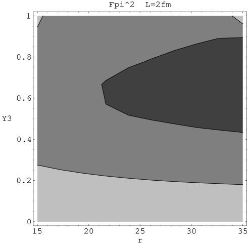
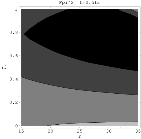
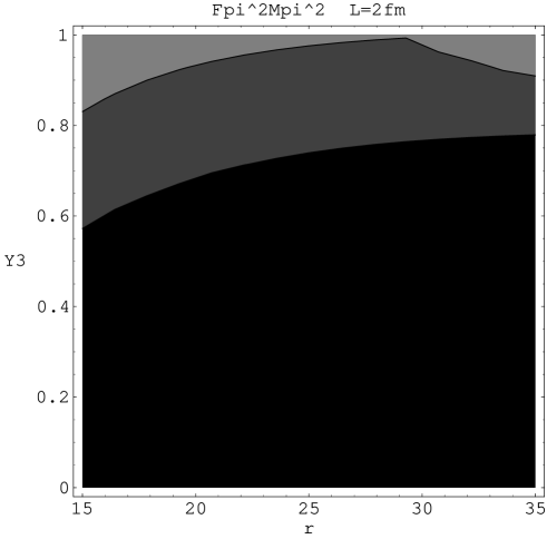
Figure 4: The maximal finite-volume corrections $D(\tilde{F}_{\pi}^{2})$ (upper plots) and $D(\tilde{F}_{\pi}^{2}\tilde{M}_{\pi}^{2})$ (lower plots) as functions of $r$ and $Y(3)$. The left (right) column corresponds to $L=2$ fm (2.5 fm). Black domains correspond to $D$ smaller than 5%, increasingly lighter domains to $D$ smaller than 10,20 and 40% respectively.

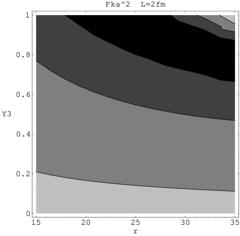
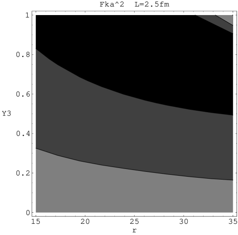
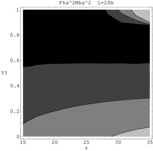
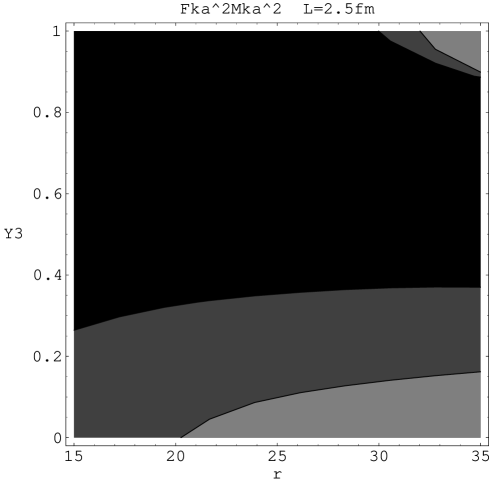
Figure 5: The maximal finite-volume corrections $D(\tilde{F}_{K}^{2})$ (upper plots) and $D(\tilde{F}_{K}^{2}\tilde{M}_{K}^{2})$ (lower plots) as functions of $r$ and $Y(3)$. The left (right) column corresponds to $L=2$ fm (2.5 fm). Black domains correspond to $D$ smaller than 5%, increasingly lighter domains to $D$ smaller than 10,20 and 40% respectively.

We observe the expected decrease of the finite-volume effects when the size of the box increases. Once again, we notice that the corrections to $F_{P}^{2}M_{P}^{2}$ are much smaller than those to the decay constants, due to a better behaviour at the approach of the infrared region. $F_{P}^{2}M_{P}^{2}$ ($P=\pi,K$) in large volumes ($L=2.5$ fm) is a quantity for which we manage a good control of finite-volume effects.

3 Constraining three-flavour order parameters on the lattice

For definiteness, we take a volume of size $L=2.5$ fm and set $r=25$. However, we must keep in mind that the latter is a parameter which may vary between 15 and approximately 35. The qualitative conclusions that we are about to draw do not depend on the exact values of $r$, but one observes small shifts in the following plots when $r$ is varied in its range.

We take into account the remainders associated with the simulated masses and decay constants $\tilde{e}_{P}$ and $\tilde{d}_{P}$ (but not the indirect remainders $d,d^{\prime},e,e^{\prime}$). As a rule of thumb resum , we estimate the size of NNLO remainders in the physical case by attributing a 30% (10%) effect to an $m_{s}$ ($m$) factor, which leads to $O(m_{s}^{2})\sim 10\%$, $O(mm_{s})\sim 3\%$ and $O(m^{2})\sim 1\%$.

For lattice simulations where $\tilde{m}$ varies, we take the following estimate:

$$\tilde{d}_{K} \sim \tilde{e}_{K}=O(\tilde{m}m_{s})\sim 0.10q^{1/3}\,,$$ (56)

$$\tilde{d}_{K} \sim \tilde{e}_{\pi}=O(m_{s}^{2})\sim 0.10\,,$$ (57)

in order to recover the physical case, i.e. $O(\tilde{m}m_{s})\simeq 0.10$ for $\tilde{m}=m_{s}$ ($q=1$) and $O(\tilde{m}m_{s})\simeq 0.03$ for $\tilde{m}=m$ ($q=1/r$).

Figs. 6 and 7 show the pseudoscalar decay constants and masses as functions of the quark mass ratio $q=\tilde{m}/m_{s}$. The left column corresponds to $Z(3)=0.8$, the right one to $Z(3)=0.4$. On each plot, the various bands show the impact of NNLO uncertainties for different values of $X(3)$ [full: 0.8, long-dashed: 0.4, dashed: 0.2]. We plot the results only when the finite-volume effects are smaller than 10%, but we do not include these corrections in the quantities plotted.

Figure 6: $\tilde{F}_{\pi}^{2}$ and $\tilde{F}_{\pi}^{2}\tilde{M}_{\pi}^{2}$ (normalised to their physical value) as functions of $q$. The first (second) column corresponds to $Z(3)=0.8$ (0.4). On each plot, full, long-dashed and dashed bands correspond respectively to $X(3)=0.8,0.4,0.2$. Cases where $Y(3)>1$ are not shown.

Figure 7: $\tilde{F}_{K}^{2}$ and $\tilde{F}_{K}^{2}\tilde{M}_{K}^{2}$ (normalised to their physical value) as functions of $q$. The first (second) column corresponds to $Z(3)=0.8$ (0.4). On each plot, full, long-dashed and dashed bands correspond respectively to $X(3)=0.8,0.4,0.2$. Cases where $Y(3)>1$ are not shown.

At small $q$, the pion mass becomes too light, the finite-volume effects become larger than 10%, and we cannot trust the corresponding results because of potentially large higher-order corrections (in such a case, we set the result to 0 on the plots). In particular the upper left plot in fig. 6 [$\tilde{F}_{\pi}^{2}/F_{\pi}^{2}$ for $Z(3)=0.8$], where $q$ must be rather large to tame finite-volume effects, confirms that the chiral expansions of the decay constants may suffer from sizeable uncertainties at small simulated masses because of large finite-volume corrections.

From the previous analysis, the sensitivity to the three-flavour order parameters through the curvature seems more important in the case of the masses (which have smaller finite-volume corrections as well). We can isolate this effect by considering the dimensionless ratios:

$$R_{\pi}=\frac{1}{q}\frac{\tilde{F}_{\pi}^{2}\tilde{M}_{\pi}^{2}}{F_{\pi}^{2}M_{\pi}^{2}}\,,\qquad\qquad R_{K}=\frac{2}{(q+1)}\frac{\tilde{F}_{K}^{2}\tilde{M}_{K}^{2}}{F_{K}^{2}M_{K}^{2}}\,.$$ (58)

Figure 8: The ratio $R_{\pi}$ as a function of $q$. The first (second) column corresponds to $r=20$ (30). The first (second) row deals with $Z(3)=0.8$ (0.4). On each plot, full, long-dashed and dashed bands correspond respectively to $X(3)=0.8,0.4,0.2$. Cases where $Y(3)>1$ are not shown.

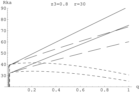
Figure 9: The ratio $R_{K}$ as a function of $q$. The first (second) column corresponds to $r=20$ (30). The first (second) row deals with $Z(3)=0.8$ (0.4). On each plot, full, long-dashed and dashed bands correspond respectively to $X(3)=0.8,0.4,0.2$. Cases where $Y(3)>1$ are not shown.

Figs. 8 and 9 indicate that these two ratios can provide a way of constraining the size of vacuum fluctuations by varying $q$ from $1/r$ to 1. The larger $r$, the easier the distinction between small and large fluctuations, even though the uncertainties due to NNLO remainders increase at the same time.

4 Conclusion

The presence of massive $s\bar{s}$-pairs in QCD vacuum may induce significant differences in the pattern of chiral symmetry breaking between $N_{f}=2$ and $N_{f}=3$ chiral limits, i.e., when $m_{s}$ remains at its physical mass and when $m_{s}$ is set to 0. This effect, related to the violation of the Zweig rule in the scalar sector, may destabilise three-flavour chiral expansions numerically, by damping leading-order (LO) terms proportional to $\Sigma(3)$ and $F^{2}(3)$, and by enhancing next-to-leading-order (NNLO) terms containing the $O(p^{4})$ Zweig-rule violating low-energy constants $L_{4}$ and $L_{6}$. In such case, a more careful treatement of chiral expansions is required to avoid uncontrolled corrections from higher chiral orders.

In a previous work resum , we proposed a consistent framework to take into account the possibility of large vacuum fluctuations. Indirect hints from dispersive estimates uuss ; uuss2 ; roypika suggest that this effect might be significant, but an experimental determination has not been achieved yet. In this paper, we proposed to probe the size of $s\bar{s}$-pairs fluctuations through lattice simulations with three dynamical flavours, with a strange quark at its physical mass $m_{s}$ and two lighter flavours of mass $\tilde{m}$. We focused on the masses and decay constants of the pions and kaons, and worked out chiral expansions which should exhibit small NNLO remainders even when LO and NLO terms compete numerically. The dependence of these observables on $\tilde{m}$ can provide useful constraints on the structure of the $N_{f}=3$ chiral vacuum, and in particular on the size of vacuum fluctuations. Conversely, this dependence on vacuum fluctuations should stand as a warning about three-flavour chiral extrapolations on the lattice, which might prove more delicate to handle than usually assumed if vacuum fluctuations of $s\bar{s}$ pairs are significant.

We have also estimated the corrections due to the finite spatial dimensions used in the lattice simulation. As expected, large volumes ($L\sim 2.5$ fm) are required to prevent these corrections from spoiling the predictivity of the chiral expansions in the $p$-regime. These corrections do not seem enhanced in the case of large vacuum fluctuations for the observables considered here.

Finally, we isolated two dimensionless ratios based on $F_{\pi}^{2}M_{\pi}^{2}$ and $F_{K}^{2}M_{K}^{2}$ showing interesting features. They are not affected very strongly by finite-volume corrections, and their dependence on $\tilde{m}$ could provide interesting insights at the size of vacuum fluctuations. Therefore, it would be rather interesting to perform a lattice study of these ratios with three dynamical flavours, a reasonably large spatial box, and an action with good chiral properties. The results might shed some light on the pattern of $N_{f}=3$ chiral symmetry breaking and the low-energy dynamics of QCD.

Appendix A Bare expansion of finite-volume tadpoles

The finite-volume tadpole $\tilde{\sigma}_{P}$ is related to its infinite-volume counterpart through $\xi_{1/2}$ which can be reexpressed as:

$$\xi_{1/2}(L,M^{2})=2\lim_{L_{t}\to\infty}g^{(4)}_{1}=\frac{1}{\sqrt{\pi}}g^{(3)}_{1/2}\,,$$ (59)

where $g^{(d)}_{r}$ has been introduced in App. A of ref. hasenleut , and the zero-temperature limit is given in eq. (B.1) of the same reference .

From App. B of ref. hasenleut , it is straightforward to determine the expansion of $g^{(3)}_{1/2}$ in powers of $M$:

$$g^{(3)}_{1/2} = \frac{1}{\sqrt{4\pi}L^{2}}\Bigg{[}\frac{2\pi}{ML}-\frac{M^{2}L^{2}}{4\pi}\log(M^{2}L^{2})$$

$$\qquad\qquad+\sum_{n=0}^{\infty}\frac{\gamma_{n}}{n!}(ML)^{2n}\Bigg{]}\,,$$

$$\gamma_{n} = \left(-\frac{1}{4\pi}\right)^{n}\left[\alpha_{n+1/2}+\frac{3}{(2n+1)(n-1)}\right]\,,\ n\neq 1\,,$$ (62)

$$\gamma_{1} = -\frac{1}{4\pi}\left[\alpha_{3/2}-\Gamma^{\prime}(1)-\log(4\pi)-\frac{5}{3}\right]\,,$$ (63)

with $\alpha_{n+1/2}$ are known numerical coefficients (the first few are displayed in table 1 of ref. hasenleut ).

This leads to the following expansion of $\xi_{1/2}(L,M)$:

$$\xi_{1/2}(L,M^{2}) = \frac{1}{ML^{3}}-\frac{M^{2}}{8\pi^{2}}\log(M^{2}L^{2})$$

$$\qquad+\frac{1}{2\pi}\sum_{n=0}^{\infty}\frac{\gamma_{n}}{n!}M^{2n}L^{2n-2}\,.$$

Thus, the nonanalytic dependence of $\tilde{\sigma}_{P}$ on ${\rm LO}(\tilde{M}_{P}^{2})$ comes only from the pole and the logarithm singled out in eq. (2.2). According to our prescription, the bare expansion is obtained once the polynomial terms are reexpanded in powers of quark masses. At our order of accuracy, this amounts to replacing $\tilde{M}_{P}^{2}$ by ${\rm LO}(\tilde{M}_{P}^{2})$ in the polynomial pieces, i.e.:

$$\frac{\tilde{\sigma}_{P}}{L^{3}} = \frac{\tilde{M}_{P}^{2}}{8\pi^{2}}\log\frac{\tilde{M}_{P}^{2}}{\mu^{2}}+\xi_{1/2}(L,\tilde{M}_{P}^{2})$$ (65)

$$\to \frac{{\rm LO}(\tilde{M}_{P}^{2})}{8\pi^{2}}\log\frac{\tilde{M}_{P}^{2}}{\mu^{2}}$$

$$\qquad+\Bigg{\{}\frac{1}{\tilde{M}_{P}L^{3}}-\frac{{\rm LO}(\tilde{M}_{P}^{2})}{8\pi^{2}}\log(\tilde{M}_{P}^{2}L^{2})$$

$$\qquad+\frac{1}{2\pi}\sum_{n=0}^{\infty}\frac{\gamma_{n}}{n!}[{\rm LO}(\tilde{M}_{P}^{2})]^{n}L^{2n-2}\Bigg{\}}$$

$$= \frac{{\rm LO}(\tilde{M}_{P}^{2})}{8\pi^{2}}\log\frac{\tilde{M}_{P}^{2}}{\mu^{2}}+\frac{1}{\tilde{M}_{P}L^{3}}$$

$$\qquad-\frac{{\rm LO}(\tilde{M}_{P}^{2})}{8\pi^{2}}\log(\tilde{M}_{P}^{2}L^{2})$$

$$\qquad+\frac{{\rm LO}(\tilde{M}_{P}^{2})}{8\pi^{2}}\log[{\rm LO}(\tilde{M}_{P}^{2})L^{2}]$$

$$\qquad+\Bigg{[}\xi_{1/2}(L,{\rm LO}(\tilde{M}_{P}^{2}))-\frac{1}{\sqrt{{\rm LO}(\tilde{M}_{P}L^{3})}}\Bigg{]}$$

$$= \frac{{\rm LO}(\tilde{M}_{P}^{2})}{8\pi^{2}}\log\frac{\tilde{M}_{P}^{2}}{\mu^{2}}+\frac{1}{\tilde{M}_{P}L^{3}}$$

$$\qquad+\frac{{\rm LO}(\tilde{M}_{P})}{8\pi^{2}}\log\frac{{\rm LO}(\tilde{M}_{P}^{2})}{\tilde{M}_{P}^{2}}$$

$$\qquad+\Bigg{[}\xi_{1/2}(L,{\rm LO}(\tilde{M}_{P}^{2}))-\frac{1}{\sqrt{{\rm LO}(\tilde{M}_{P})L^{3}}}\Bigg{]}\,.$$

The bracketed term has only a polynomial dependence on ${\rm LO}(\tilde{M}_{P}^{2})$. This expression yields eq. (2.2) and the bare expansion of $\tilde{\sigma}_{P}$.

References

(1)
S. Descotes-Genon, L. Girlanda and J. Stern,
JHEP 0001, 041 (2000)
[hep-ph/9910537].
(2)
H. Leutwyler and A. Smilga,
Phys. Rev. D 46 (1992) 5607.
S. Descotes-Genon and J. Stern,
Phys. Rev. D 62, 054011 (2000)
[hep-ph/9912234].
(3)
J. Stern,
hep-ph/9801282.
(4)
S. Pislak et al. [BNL-E865 Collaboration],
Phys. Rev. Lett. 87 (2001) 221801
[hep-ex/0106071];
Phys. Rev. D 67 (2003) 072004
[hep-ex/0301040].
(5)
B. Ananthanarayan, G. Colangelo, J. Gasser and H. Leutwyler,
Phys. Rept. 353 (2001) 207
[hep-ph/0005297].
(6)
S. Descotes-Genon, N. H. Fuchs, L. Girlanda and J. Stern,
Eur. Phys. J. C 24, 469 (2002)
[hep-ph/0112088].
(7)
G. Colangelo, J. Gasser and H. Leutwyler,
Phys. Rev. Lett. 86 (2001) 5008
[hep-ph/0103063].
(8)
J. Gasser and H. Leutwyler,
Annals Phys. 158 (1984) 142.
(9)
J. Gasser and H. Leutwyler,
Nucl. Phys. B 250 (1985) 465.
(10)
S. Descotes-Genon and J. Stern,
Phys. Lett. B 488, 274 (2000)
[hep-ph/0007082].
(11)
B. Moussallam,
Eur. Phys. J. C 14 (2000) 111
[hep-ph/9909292];
JHEP 0008 (2000) 005
[hep-ph/0005245].
S. Descotes-Genon,
JHEP 0103 (2001) 002
[hep-ph/0012221].
(12)
P. Büttiker, S. Descotes-Genon and B. Moussallam,
Eur. Phys. J. C 33 (2004) 409
[hep-ph/0310283].
(13)
G. Amoros, J. Bijnens and P. Talavera,
Nucl. Phys. B 568 (2000) 319
[hep-ph/9907264].
J. Bijnens, P. Dhonte and P. Talavera,
JHEP 0401 (2004) 050
[hep-ph/0401039];
JHEP 0405 (2004) 036
[hep-ph/0404150].
(14)
J. Bijnens and P. Dhonte,
JHEP 0310 (2003) 061
[hep-ph/0307044].
(15)
S. Descotes-Genon, N. H. Fuchs, L. Girlanda and J. Stern,
Eur. Phys. J. C 34, 201 (2004)
[hep-ph/0311120].
(16)
K. Ishikawa, Hadron spectrum from dynamical simulations,
plenary talk at the 22nd International Symposium
on Lattice Field Theory (Lattice 2004), Batavia, Illinois,
21-26 Jun 2004,
hep-lat/0410050.
(17)
J. Gasser and H. Leutwyler,
Phys. Lett. B 184 (1987) 83;
Phys. Lett. B 188 (1987) 477;
Nucl. Phys. B 307 (1988) 763.
H. Leutwyler,
Phys. Lett. B 189 (1987) 197.
(18)
M. Luscher,
Commun. Math. Phys. 104 (1986) 177.
(19)
D. Becirevic and G. Villadoro,
Phys. Rev. D 69, 054010 (2004)
[hep-lat/0311028].
G. Colangelo and S. Dürr,
Eur. Phys. J. C 33, 543 (2004)
[hep-lat/0311023].
G. Colangelo and C. Haefeli,
Phys. Lett. B 590, 258 (2004)
[hep-lat/0403025].
(20)
P. Hasenfratz and H. Leutwyler,
Nucl. Phys. B 343 (1990) 241.