Neutral Pion-like Resonances at Photon Colliders

Abstract

Two photons can annihilate into a neutral pion-like resonance via the anomaly coupling, just like $\pi^{0}\gamma\gamma$ in QCD. In some strongly interacting electroweak symmetry breaking models, e.g., technicolor type models, there often exist neutral pion-like resonances. TeV photon colliders have a strong capability to discover such particles, because the standard model background in photon scattering goes through box diagrams and is therefore highly suppressed. In this study, we perform a signal-background comparison. We show that $e^{+}e^{-}$ linear colliders running in $\gamma\gamma$ mode can discover such neutral-pion-like resonances with a decent sensitivity.

I Introduction

The major goal of the next generation collider experiments is to explore the mechanism of electroweak symmetry breaking (EWSB). In the standard model (SM), a Higgs doublet field is responsible for EWSB and gives rise to an elementary Higgs boson. However, the gauge hierarchy problem arises from the fact that the radiative correction to the Higgs boson mass has a quadratic divergence, which demands a finely tuned cancellation of order of $10^{-16}$ between the bare mass term and the correction terms. Such a fine tuning problem has motivated a lot of new physics. A particular class of solutions involves some strong dynamics at the TeV scale. The Higgs boson could then be replaced by a condensate due to the new dynamics. Technicolor TC ; walk , topcolor topcolor , and topcolor assisted technicolor ttc models are typical examples of this kind. The recent Higgsless models also become strongly coupled at a few TeV nomura where some strong dynamics appears.

One of the new features of these strongly interacting models is the existence of new mesons and baryons bounded by the new interactions. In technicolor models often singlets and doublets of techni-fermions are proposed. These techni-fermions can form bound states via the technicolor interactions. If the normal QCD theory is borrowed and rescaled to the electroweak scale, we would have many techni-mesons and techni-baryons. As in QCD the neutral pion $\pi^{0}$ is very unique because of the anomaly coupling, through which the $\pi^{0}$ decays into a pair of photons almost 100%. Therefore, in technicolor models there are also neutral techni-pions that couples to a pair of gauge bosons via the anomaly couplings, in particular the coupling to a pair of photons. In collider experiments, the neutral techni-pion once produced will decay into a pair of photons with a sharp invariant-mass peak, which is a very unique signature for neutral techni-pions. Here we consider two photon collisions at TeV scale, which is very unique in probing for some neutral pion-like resonances of some new physics models. Some previous studies of technimesons at photon collisions can be found in Refs. oldref .

In one simple technicolor model, the Technicolor Straw Man model straw , the lightest techni-mesons are constructed solely from the lightest techni-fermion doublet $(T_{U},T_{D})$, from which isotriplets $\rho_{T}^{0,\pm},\pi_{T}^{0,\pm}$ and isosinglets $\pi^{{}^{\prime}0}_{T},\,\omega^{0}_{T}$ can be formed. In particular, the neutral $\pi^{0}_{T}$ and $\pi^{{}^{\prime}0}_{T}$ have an anomaly-type coupling to a pair of photons as shown in Fig. 1.

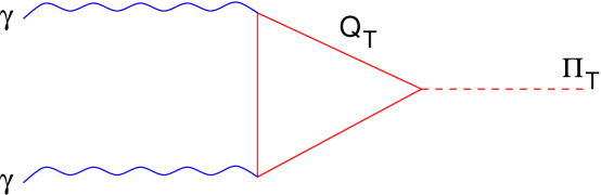
Figure 1: Feynman diagram for the anomaly-type coupling of the neutral techni-pion.

In this paper, we specifically work on two models: (i) a rescaled QCD model rescale and (ii) the low-scale technicolor model low . In the rescaled QCD model, the anomaly coupling of the techni-pion $\pi^{0}_{T}$ is the rescaled version of the usual QCD, i.e., the $\pi^{0}$ decay constant is rescaled by the factor $v/f_{\pi^{0}}$, where $v=246$ GeV and $f_{\pi^{0}}=130$ MeV pdg . In this particular rescaled QCD model, the $\pi^{0}_{T}$ couples to $\gamma\gamma$, $\gamma Z$, and $ZZ$ through the anomaly. We will give more details and formulas in the next section.

In the low-scale technicolor model that we consider is a multi-scale technicolor model low . Quark and lepton masses are generated by broken extended technicolor gauge interactions in the walking technicolor modelwalk . The walking technicolor coupling runs very slowly up to the extended technicolor gauge scale (a few hundred TeV) by including a large number of techni-fermions. Such a slowly running coupling allows quark and lepton masses as large as a few GeV to be generated by the extended technicolor gauge interactions at a few hundred TeV scale. There are two types of techni-fermions that condense at widely separated scales. The upper scale is set by $v=246$ GeV while the low scale is roughly given by $f_{\pi_{T}}=v/\sqrt{N_{D}}$, where $N_{D}$ is the number of techni-fermion doublets. The techni-hadrons associated with the low scale are of immediate interests at colliders. Note that the extended technicolor gauge interaction only generates a few GeV to the top quark. The top mass is, however, generated by another so called topcolor interaction topcolor . The techni-pions will couple to normal quarks and leptons through the extended technicolor gauge interactions. The couplings are Higgs-like however, and so the neutral techni-pion will decay into the heaviest possible fermion pair, e.g.,

$$\pi_{T}^{0}\to b\bar{b}\;\;\;{\rm or}\;\;\;t\bar{t}\;,$$

depending on the mass of the techni-pion. Thus, the decay of the neutral techni-pion in this model also includes $gg$, $b\bar{b}$, $c\bar{c}$, etc.

The organization is as follows. In the next section, we describe the production of and in Sec. III the decay of the neutral techni-pion in the rescaled QCD model and the low-scale technicolor model in photon collisions. We conclude in Sec. IV.

II Production

The general form of the anomaly coupling of the neutral techni-pion $\pi^{0}_{T}$ to two gauge bosons $G_{1},G_{2}$ is given by

$${\cal M}=N_{TC}{\cal A}_{G_{1}G_{2}}\frac{g_{1}g_{2}}{2\pi^{2}f_{\pi_{T}}}\,\epsilon_{\nu}\epsilon_{\lambda}\epsilon^{\nu\lambda\alpha\beta}P_{1\alpha}P_{2\beta}\;,$$ (1)

where $\epsilon_{\nu}(P_{1})$ and $\epsilon_{\lambda}(P_{2})$ are the polarization 4-vector of the gauge bosons $G_{1}$ and $G_{2}$, respectively. Here ${\cal A}_{G_{1}G_{2}}$ is the anomaly factor, $N_{TC}$ is the number of technicolors, $g_{i}$’s are the gauge couplings of the gauge bosons, and $f_{\pi_{T}}=\frac{v}{\sqrt{N_{D}}}$ is the decay constant of the techni-pion. The differential cross section for $\gamma\gamma\to\pi^{0}_{T}$ is given by

$$d\hat{\sigma}=\frac{1}{2\hat{s}}\overline{\sum}\left|{\cal M}\right|^{2}(2\pi)^{4}\delta^{(4)}(P_{1}+P_{2}-P_{\pi_{T}})\;\frac{d^{3}\vec{P}_{\pi_{T}}}{(2\pi)^{3}2P^{0}_{\pi_{T}}}\;,$$ (2)

where $P_{1}$, $P_{2}$, and $P_{\pi_{T}}$ are the 4-momenta of the incoming photons and the outgoing $\pi^{0}_{T}$, respectively, $\overline{\sum}|{\cal M}|^{2}$ is the spin-averaged amplitude squared, and $\hat{s}=(P_{1}+P_{2})^{2}$. The scattering amplitude for $\gamma\gamma\to\pi^{0}_{T}$ is obtained from Eq. (1) by specifying the gauge group:

$$i{\cal M}(\gamma\gamma\to\pi_{T}^{0})=iN_{TC}{\cal A}_{\gamma\gamma}\frac{e^{2}}{2\pi^{2}f_{\pi_{T}}}\epsilon_{\nu}(P_{1})\epsilon_{\lambda}(P_{2})\epsilon^{\nu\lambda\alpha\beta}P_{1\alpha}P_{2\beta}\;.$$ (3)

After squaring and averaging over initial polarizations, we obtain

$$\overline{\sum}\left|{\cal M}\right|^{2}=\frac{1}{2}\left(N_{TC}{\cal A}_{\gamma\gamma}\frac{e^{2}}{\pi^{2}f_{\pi_{T}}}\right)^{2}(\hat{s}/4)^{2}\;.$$ (4)

We can then integrate to obtain the cross section as

$$\hat{\sigma}(\gamma\gamma\to\pi_{T}^{0})=\frac{\pi m_{\pi_{T}}}{64}\left(N_{TC}{\cal A}_{\gamma\gamma}\frac{e^{2}}{\pi^{2}f_{\pi_{T}}}\right)^{2}\delta^{(0)}(\sqrt{\hat{s}}-m_{\pi_{T}})\;.$$ (5)

To obtain the realistic cross section $\sigma(\gamma\gamma\to\pi_{T}^{0})$ at an $e^{+}e^{-}$ collider, we convolute the subprocess cross section $\hat{\sigma}(\gamma\gamma\to\pi_{T}^{0})$ with the photon luminosity function,

$$\sigma(\gamma\gamma\to\pi_{T}^{0})=\int_{x_{1min}}^{x_{max}}\!\int_{x_{2min}}^{x_{max}}F_{\gamma/e}(x_{1})F_{\gamma/e}(x_{2})\hat{\sigma}(\gamma\gamma\to\pi_{T}^{0};\;\hat{s}=x_{1}x_{2}s)dx_{1}dx_{2}\;.$$ (6)

In this paper, $\sqrt{s}$ always refers to the center-of-mass energy of the parent $e^{+}e^{-}$ collider and $\sqrt{\hat{s}}$ always refers to the total energy of the two incoming photons. The laser backscattering laser is the standard technique to efficiently convert an electron beam into a photon beam. The resulting photon luminosity function $F_{\gamma/e}(x_{i})$ is given by km

$$F_{\gamma/e}(x_{i})=\frac{1}{D(\xi)}\left[1-x_{i}+\frac{1}{1-x_{i}}-\frac{4x_{i}}{\xi(1-x_{i})}+\frac{4x_{i}^{2}}{\xi^{2}(1-x_{i})^{2}}\right]\;,$$ (7)

where $D(\xi)=(1-\frac{4}{\xi}-\frac{8}{\xi^{2}})\ln(1+\xi)+\frac{1}{2}+\frac{8}{\xi}-\frac{1}{2(1+\xi)^{2}}$ and $\xi\simeq 4.8$ in this case for maximal energy conversion. Finally, the cross section is

$$\sigma(\gamma\gamma\to\pi_{T}^{0})=\frac{m_{\pi_{T}}^{2}}{2^{5}s\pi^{3}}(\frac{N_{TC}{\cal A}_{\gamma\gamma}e^{2}}{f_{\pi_{T}}})^{2}\;\int_{x_{min}}^{x_{max}}\frac{1}{x}F_{\gamma/e}(x)F_{\gamma/e}(\frac{m_{\pi_{T}}^{2}}{sx})dx\;.$$ (8)

In the following, we specifically work on the two models that we described. The difference between the rescaled model and the low-scale model lies in the anomaly factor ${\cal A}_{G_{1}G_{2}}$:

$${\cal A}_{G_{1}G_{2}}=Tr[T^{a}(\{T_{1},T_{2}\}_{L}+\{T_{1},T_{2}\}_{R})]\;,$$ (9)

where $T_{i}$ is the generator associated with the gauge boson $G_{i}$, and $T^{a}$ is the generator of the axial current associated with the techni-pion

$$j^{\mu 5a}=\bar{\psi}\gamma^{\mu}\gamma^{5}T^{a}\psi\;.$$ (10)

The values of ${\cal A}_{G_{1}G_{2}}$ for the rescaled model are essentially the same as the usual QCD while the low-scale model involves different values of charges. Specifically for ${\cal A}_{\gamma\gamma}$, we have

$${\cal A}_{\gamma\gamma}=Tr(T^{a}Q^{2})=\left\{\begin{array}[]{ll}\frac{1}{6}&\mbox{ for the rescaled model}\\ \frac{5}{6}&\mbox{ for the low-scale model}\end{array}\right.\;,$$ (11)

which is the consequence of the assignment of charges $Q$. The electric charge $Q$ of the techni-fermions $T_{U}$ and $T_{D}$ is

$$Q=\left(\begin{array}[]{cc}Q_{u}&0\\ 0&Q_{d}\end{array}\right)\;,$$

where $Q_{u}$ and $Q_{d}$ have different values for the two models:

	$Q_{u}$	$Q_{d}$
rescaled	$2/3$	$-1/3$
low-scale	$4/3$	$1/3$

III Decay

Next we have to consider the final states into which the techni-pion decays. Through the anomaly couplings the neutral techni-pion can decay into $\gamma\gamma,\,\gamma Z,\,ZZ$ ($gg$ mode is absent if the internal techni-fermions do not carry color.) We particularly choose the $\gamma\gamma$ final state because of the larger branching ratio and the fact that photon does not involve further decay in the detection. The cross section of $\gamma\gamma\to\pi^{0}_{T}\to\gamma\gamma$ is given by, in the on-shell approximation,

$$\sigma(\gamma\gamma\to\pi_{T}^{0}\to\gamma\gamma)=\sigma(\gamma\gamma\to\pi_{T}^{0})\Gamma(\pi_{T}^{0}\to\gamma\gamma)$$ (12)

which is valid because the width $\Gamma(\pi^{0}_{T}\to\gamma\gamma)$ is very narrow. This is a very interesting process because the signal is a tree-level process while the SM background has to go through box diagrams box , which are naturally suppressed.

Let us first evaluate the branching ratio of $\pi^{0}_{T}\to\gamma\gamma$. In the rescaled model, the total width is the sum of $\Gamma(\pi^{0}_{T}\to\gamma\gamma)$, $\Gamma(\pi^{0}_{T}\to\gamma Z)$, and $\Gamma(\pi^{0}_{T}\to ZZ)$:

$$\Gamma_{total} = \frac{c^{2}m_{\pi_{T}}^{3}}{2^{6}\pi}+\frac{c_{1}^{2}(m_{\pi_{T}}^{2}-m_{Z}^{2})^{3}}{2^{4}\pi m_{\pi_{T}}(m_{\pi_{T}}^{2}+m_{Z}^{2})}+\frac{c_{2}^{2}(m_{\pi_{T}}^{2}-4m_{Z}^{2})^{2}}{2^{4}\pi m_{\pi_{T}}}$$ (13)

$$= \frac{1}{2^{4}\pi m_{\pi_{T}}}\left[\frac{c^{2}m_{\pi_{T}}^{4}}{2^{2}}+\frac{c_{1}^{2}(m_{\pi_{T}}^{2}-m_{Z}^{2})^{3}}{(m_{\pi_{T}}^{2}+m_{Z}^{2})}+c_{2}^{2}(m_{\pi_{T}}^{2}-4m_{Z}^{2})^{2}\right]$$

where $c=N_{TC}{\cal A}_{\gamma\gamma}\frac{e^{2}}{2\pi^{2}f_{\pi_{T}}}$, $c_{1}=N_{TC}{\cal A}_{\gamma Z}\frac{eg_{Z}}{2\pi^{2}f_{\pi_{T}}}$, $c_{2}=N_{TC}{\cal A}_{ZZ}\frac{g^{2}_{Z}}{2\pi^{2}f_{\pi_{T}}}$, and

$${\cal A}_{\gamma\gamma} = Tr(T^{a}Q^{2})$$

$${\cal A}_{\gamma Z} = Tr[T^{a}(T_{3L}+T_{3R}-2Q\sin^{2}\theta_{w})Q]$$

$${\cal A}_{ZZ} = Tr[T^{a}((T_{3L}-Q\sin^{2}\theta_{w})^{2}+(T_{3R}-Q\sin^{2}\theta_{w})^{2})]\;.$$

The assignment of $Q$ for the two models has been shown in the above.

In the low-scale model, we must consider another important mode, $\pi^{0}_{T}\to b\bar{b}$, the decay width of which is given by straw

$$\left.\Gamma(\pi_{T}^{0}\to b\bar{b})\right|_{\rm low-scale}=\frac{1}{16\pi f_{\pi_{T}}^{2}}N_{b}P_{b}C^{2}_{1b}(m_{b}+m_{b})^{2}$$ (14)

where $N_{b}=3$, $P_{b}$ is the momentum of the $b$ quark, and $C_{1b}$ is a model dependent parameter of order $O(1)$ but the topcolor-assisted technicolor suggested that $C_{1t}\lesssim m_{b}/m_{t}$, which means the $t\bar{t}$ mode is suppressed. We show the branching ratio $B(\pi^{0}_{T}\to\gamma\gamma)$ versus the techni-pion mass in Fig. 2. The rescaled and low-scale models are shown. The branching ratio $B(\pi^{0}_{T}\to\gamma\gamma)$ for the rescaled model decreases with $m_{\pi_{T}}$ because the $\gamma Z$ and $ZZ$ modes become less suppressed in the phase space. It eventually approaches a stable value when the techni-pion mass becomes very large. On the other hand, $B(\pi^{0}_{T}\to\gamma\gamma)$ for the low-scale model increases with $m_{\pi_{T}}$ because the $b\bar{b}$ width roughly scales as $m_{\pi_{T}}$ while the $\gamma\gamma$ width scales as $m^{3}_{\pi_{T}}$.

Figure 2: Branching ratio $B(\pi^{0}_{T}\to\gamma\gamma)$ of the techni-pion versus the techni-pion mass for (a) the rescaled model and (b) the low-scale model.

We are now ready to compare the signal cross sections with the SM background. They are shown in Fig. 3 for both the rescaled and low-scale models, as well as the SM $\gamma\gamma\to\gamma\gamma$ background box . Some specific choices for $N_{TC}$ and $N_{D}$ are made. The cross section $\sigma$ scales with $N_{TC}^{2}$ and with $N_{D}$. We have also imposed kinematical cuts:

$$\frac{M_{\gamma\gamma}}{\sqrt{s_{ee}}}>0.3,\;\;\;|\cos\theta_{\gamma}|<\cos 30^{\circ}$$

in order to suppress the background, which is very forward and has a continuous $M_{\gamma\gamma}$ spectrum. The SM background is of order of $O(10)$ fb for $\sqrt{s}_{ee}=0.5-2.0$ TeV. From Fig. 3 the rescaled model gives a curve which increases very mildly with the techni-pion mass. This is because the production cross section increases with $m_{\pi_{T}}$ (see Eq. (8)) but the branching ratio of $\pi^{0}_{T}\to\gamma\gamma$ decreases with $m_{\pi_{T}}$ (see Fig. 2). On the other hand, the low-scale model gives a curve that increases much more rapidly because the branching ratio of $\pi^{0}_{T}\to\gamma\gamma$ also increases with $m_{\pi_{T}}$ (see Fig. 2.) Here we have chosen $N_{TC}=4$ and $N_{D}=3$. Note that $f_{\pi_{T}}=v/\sqrt{N_{D}}$. Both curves eventually dip down at the upper end because of limitation on the phase space. It is clear that for a reasonable choice of parameters the techni-pion signal is rather clean relative to the standard model background. In addition, the signal cross section is a few fb to $O(10)$ fb. The event rate with $O(100)$ fb^-1 luminosity is high enough for a feasible search for this kind of signal. If we are to quantify the significance of the signal, we can use $S/\sqrt{B}$, where $S$ and $B$ are the number of the signal and background events, respectively. With an integrated luminosity of 100 fb^-1 a signal cross section of 2 fb and a background of 10 fb will give a significance of $6.3$. Therefore, all the cross sections shown in Fig. 3 being larger than 2 fb will give sufficiently significant signals. Furthermore, the signal will be a sharp peak determined by the experimental resolution (the intrinsic width is very small) and above the continuum background.

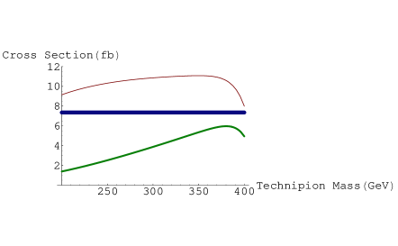
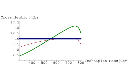
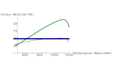
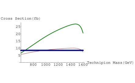
Figure 3: Production cross sections for the techni-pions of the rescaled model (the thin slant line, brown in color) and of the low-scale model (the thick slant line, the green line) and the SM background (the horizontal blue line) versus the techni-pion mass at $e^{+}e^{-}$ linear colliders running in laser backscattering mode. (a) $\sqrt{s}_{ee}=500$ GeV, (b) $\sqrt{s}_{ee}=1000$ GeV, (c) $\sqrt{s}_{ee}=1500$ GeV, and (d) $\sqrt{s}_{ee}=2000$ GeV. We have used $N_{TC}=4$, $N_{D}=3$, and imposed the kinematic cuts as $\frac{M_{\gamma\gamma}}{\sqrt{s}_{ee}}>0.3$ and $|\cos\theta_{\gamma}|<\cos 30^{\circ}$.

IV Conclusions

We have pointed out that the TeV photon-photon collider is very special in probing for $O({\rm TeV})$ neutral pion-like resonances, which have a anomaly coupling to a pair of photons. Many extensions of the SM predict the existence of such resonances. Famous examples are technicolor models or variants of technicolor models. The advantage of low SM background makes photon colliders very unique in searching for neutral pion-like resonances.

References

- (1) S. Weinberg, Phys. Rev. D19, 1277 (1979); L. Susskind, Phys. Rev. D20, 2619 (1979); E. Eichten and K. Lane, Phys. Lett. B90, 125 (1980).
- (2) B. Holdom, Phys. Rev. D24, 1441 (1981); T. Appelquist, D. Karabali, and L. Wijewardhana, Phys. Rev. Lett.57, 957 (1986); K. Yamawaki, M. Bando, and K. Matumoto, Phys. Rev. Lett. 56, 1335 (1986); T. Akiba and T. Yanagida, Phys. Lett. B169, 432 (1986).
- (3) C. T. Hill, Phys. Lett. B266, 419 (1991).
- (4) C. T. Hill, Phys. Lett. B345, 483 (1995); K. Lane and E. Eichten, Phys. Lett. B352, 382 (1995).
- (5) Y. Nomura, JHEP 0311, 050 (2003).
- (6) J. Tandean, Phys. Rev. D52, 1398 (1995); J.A. Grifols, Phys. Lett. B102, 277 (1981).
- (7) K. Lane and S. Mrenna, Phys. Rev. D67, 115011 (2003). K. Lane (Boston U.), hep-ph/9903372.
- (8) K. Lynch and E. Simmons, Phys. Rev. D64, 035008 (2001).
- (9) E. Eichten and K. Lane, Phys. Lett. B388, 803 (1996); E. Eichten, K. Lane, and J. Womersley, Phys. Lett. B405, 305 (1997).
- (10) Particle Data Group, S. Eidelman et al., Phys. Lett. B592, 1 (2004)
- (11) V. Telnov, eConf C010630:E3026,2001; Nucl. Instrum. Meth. A355, 3 (1995).
- (12) See e.g., K. Cheung, Phys. Rev. D47, 3750 (1993).
- (13) G. Gounaris, P. Porfyriadis, and F. Renard, Eur. Phys. J. C9, 673 (1999).