CPT-2004/P.017

Abstract

We extend the earlier suggested QCD-motivated model for the $Q^{2}$-dependence of the generalized Gerasimov-Drell-Hearn (GDH) sum rule which assumes the smooth dependence of the structure function $g_{T}$, while the sharp dependence is due to the $g_{2}$ contribution and is described by the elastic part of the Burkhardt-Cottingham sum rule. The model successfully predicts the low crossing point for the proton GDH integral, but is at variance with the recent very accurate JLAB data. We show that, at this level of accuracy, one should include the previously neglected radiative and power QCD corrections, as boundary values for the model. We stress that the GDH integral, when measured with such a high accuracy achieved by the recent JLAB data, is very sensitive to QCD power corrections. We estimate the value of these power corrections from the JLAB data at $Q^{2}\sim 1\mbox{GeV}^{2}$. The inclusion of all QCD corrections leads to a good description of proton, neutron and deuteron data at all $Q^{2}$.

PACS numbers: 11.55.Hx, 13.60.Hb, 13.88.+e

The generalized ($Q^{2}$-dependent) Gerasimov-Drell-Hearn (GDH) sum rules [1, 2] are just being tested experimentally for proton, neutron and deuteron [3, 4, 5, 6]. The characteristic feature of the proton data is the strong dependence on the four-momentum transfer $Q^{2}$, for $Q^{2}<1\mbox{GeV}^{2}$, with a zero crossing for $Q^{2}\sim 200-250\mbox{MeV}^{2}$, which is in complete agreement with our prediction [7, 8], published almost 10 years ago. Our approach is making use of the relation to the Burkhardt-Cottingham sum rule for the structure function $g_{2}$, whose elastic contribution is the main source of a strong $Q^{2}$-dependence, while the contribution of the other structure function, $g_{T}=g_{1}+g_{2}$ is smooth.

However, the recently published proton JLAB data [6] lie below the prediction, displaying quite a similar shape. Such a behaviour suggests, that the reason for the discrepancy may be the oversimplified treatment of the QCD expressions at the boundary point $Q_{0}\sim 1\mbox{GeV}$, defined in the smooth interpolation between large $Q^{2}$ and $Q^{2}=0$ and which serve as an input for our model. For large $Q^{2}$ we took the asymptotic value for the GDH integral and we neglected all the calculable corrections, as well as the contribution of the $g_{2}$ structure function. This was quite natural and unnecessary 10 years ago, since no data was available at that time.

In the present paper we fill this gap and include the radiative (logarithmic) and power QCD corrections. We found that the JLAB data are quite sensitive to power corrections and may be used for the extraction of the relevant phenomenological parameters. We present here the numerical values of these parameters which naturally depend on the approximation of the QCD perturbation theory. The resulting theoretical uncertainty should be of order of the last term of the perturbative series , taken into account, and should not therefore be more than several percents.

Moreover, the perturbative series should contain the renormalon ambiguity due to the factorial growth of the coefficients, resulting in a power rather than logarithmic correction with an unspecified coefficient. It is in fact this ambiguity which allows the interpretation of the dependence of the numerical value of the power correction, earlier mentioned for the case of the $F_{3}$ structure function [9], as an ambiguity in the separation of logarithmic and power corrections.

We use the values of the power corrections as an input for our model at $Q_{0}^{2}\sim 1\mbox{GeV}^{2}$ and we achieve a rather good description of the proton data at lower $Q^{2}$. We also present the improved description of the neutron and deuteron data and the behaviour of the Bjorken sum rule at low $Q^{2}$.

The starting point of our approach is the analysis of the general tensor structure of $W^{\mu\nu}_{A}$, the spin-dependent part of hadronic tensor $W^{\mu\nu}$. It is a linear combination of all possible Lorentz-covariant tensors, which should be orthogonal to the virtual photon momentum $q$, as required by gauge invariance, and linear in the nucleon covariant polarization $s$, from a general property of the density matrix. If the nucleon has momentum $p$, we have as usual, $s\cdot p=0$ and $s^{2}=-1$. There are only two such tensors: the first one arises already in the Born diagram

$$T_{1}^{\mu\nu}=\epsilon^{\mu\nu\alpha\beta}s_{\alpha}q_{\beta}$$ (1)

and the second tensor is just

$$T_{2}^{\mu\nu}=(s\cdot q)\epsilon^{\mu\nu\alpha\beta}p_{\alpha}q_{\beta}~{}.$$ (2)

The scalar coefficients of these tensors are specified in a well-known way, since we have

$$W^{\mu\nu}_{A}={-i\epsilon^{\mu\nu\alpha\beta}\over{p\cdot q}}q_{\beta}(g_{1}(x,Q^{2})s_{\alpha}+g_{2}(x,Q^{2})(s_{\alpha}-p_{\alpha}{s\cdot q\over{p\cdot q}}))=$$

$${-i\epsilon^{\mu\nu\alpha\beta}\over{p\cdot q}}q_{\beta}((g_{1}(x,Q^{2})+g_{2}(x,Q^{2}))s_{\alpha}-g_{2}(x,Q^{2})p_{\alpha}{s\cdot q\over{p\cdot q}})~{}.$$ (3)

Therefore, due to the factor $(s\cdot q)$, $g_{2}$ is making the difference between longitudinal and transverse polarizations, while $g_{T}=g_{1}+g_{2}$ contributes equally in both cases.

Let us consider now the $Q^{2}$-dependent integral

$$I_{1}(Q^{2})={2M^{2}\over{Q^{2}}}\Gamma_{1}(Q^{2})\equiv{2M^{2}\over{Q^{2}}}\int^{1}_{0}g_{1}(x,Q^{2})dx~{}.$$ (4)

It is defined for all $Q^{2}$, and $g_{1}(x,Q^{2})$ is the obvious generalization for all $Q^{2}$ of the standard scale-invariant structure function $g_{1}(x)$. Note that the elastic contribution at $x=1$ is not included in the above sum rule. Then, by changing the integration variable $x\to Q^{2}/2M\nu$, one recovers at $Q^{2}=0$ the integral over all energies of spin-dependent photon-nucleon cross-section, whose value is defined by the GDH sum rule [1, 2]

$$I_{1}(0)=-{\mu_{A}^{2}\over 4}~{},$$ (5)

where $\mu_{A}$ is the nucleon anomalous magnetic moment in nuclear magnetons. While $I_{1}(0)$ is always negative, its value at large $Q^{2}$ is determined by the $Q^{2}$ independent integral $\int^{1}_{0}g_{1}(x)dx$, which is positive for the proton and negative for the neutron.

The separation of the contributions of $g_{T}$ and $g_{2}$ leads to the decomposition of $I_{1}(Q^{2})$ as the difference between $I_{T}(Q^{2})$ and $I_{2}(Q^{2})$

$$I_{1}(Q^{2})=I_{T}(Q^{2})-I_{2}(Q^{2}),$$ (6)

where

$$I_{T}(Q^{2})={2M^{2}\over{Q^{2}}}\int^{1}_{0}g_{T}(x,Q^{2})dx,\;\;\;\;I_{2}(Q^{2})={2M^{2}\over{Q^{2}}}\int^{1}_{0}g_{2}(x,Q^{2})dx~{}.$$ (7)

There are solid theoretical arguments to expect a strong $Q^{2}$-dependence of $I_{2}(Q^{2})$. It is the well-known Burkhardt-Cottingham sum rule [10]. It states that

$$I_{2}(Q^{2})={1\over 4}\mu G_{M}(Q^{2})\frac{\mu G_{M}(Q^{2})-G_{E}(Q^{2})}{1+Q^{2}/4M^{2}},$$ (8)

where $\mu$ is the nucleon magnetic moment, $G_{M}(Q^{2})$ and $G_{E}(Q^{2})$ denote the familiar Sachs form factors, which are dimensionless and normalized to unity at $Q^{2}=0$, $G_{M}(0)=G_{E}(0)=1$. For large $Q^{2}$, as a consequence of the $Q^{2}$ behavior of the r.h.s. of Eq. (8), we get

$$\int^{1}_{0}g_{2}(x,Q^{2})dx=0.$$ (9)

In particular, from Eq. (9) it follows that

$$I_{2}(0)={\mu_{A}^{2}+\mu_{A}e\over 4},$$ (10)

$e$ being the nucleon charge in elementary units. To reproduce the GDH value (see Eq. (5)) one should have

$$I_{T}(0)={\mu_{A}e\over 4},$$ (11)

which was indeed proved by Schwinger [11]. The importance of the $g_{2}$ contribution can be seen already, since the entire $\mu_{A}$-term for the GDH sum rule is provided by $I_{2}$.

Note that $I_{T}$ does not differ from $I_{1}$ for large $Q^{2}$ due to the BC sum rule, but it is positive in the proton case. It is possible to obtain a smooth interpolation for $I^{p}_{T}(Q^{2})$ between large $Q^{2}$ and $Q^{2}=0$ [7]

$$I^{p}_{T}(Q^{2})=\theta(Q^{2}_{0}-Q^{2})({\mu_{A,p}\over 4}-{2M^{2}Q^{2}\over{(Q^{2}_{0})^{2}}}\Gamma^{p}_{1})+\theta(Q^{2}-Q^{2}_{0}){2M^{2}\over{Q^{2}}}\Gamma^{p}_{1},$$ (12)

where $\Gamma^{p}_{1}=\int^{1}_{0}g^{p}_{1}(x)dx$. The continuity of the function and of its derivative is guaranteed with the choice $Q^{2}_{0}=(16M^{2}/\mu_{A,p})\Gamma^{p}_{1}\sim\mbox{1GeV}^{2}$, where the integral is given by the world average proton data.

This smooth interpolation seems to be very reasonable in the framework of the QCD sum rules method [8, 12], as the low energy theorem for the quantity linear in $\mu_{A}$ may, in principle, be obtained by making use of Ward identities. It is also compatible with resonance approaches [13], as we observed earlier [8] that the magnetic transition to $\Delta(1232)$, being the main origin of sharp dependence in that approach, contributes only to $g_{2}$.

However, such interpolation neglects the QCD perturbative and power corrections and on the other hand, it assumes that at the boundary point $Q_{0}$ the contribution of $g_{2}$ is already extremely small so that

$$I^{p}_{T}(Q_{0}^{2})=I^{p}_{1}(Q_{0}^{2}).$$ (13)

Both types of corrections are easily taken into account, although this does not allow a simple analytic parametrization.

The starting point of the upgraded model is the corrected expression for the asymptotic expression for $I_{1}^{i}$ ($i=p,n$):

$$I_{1}^{i}(Q^{2})={2M^{2}\over{Q^{2}}}[\int^{1}_{0}g_{1}^{i}(x,Q^{2})dx(1-\frac{\alpha_{s}(Q^{2})}{2\pi})-c_{i}\frac{<<O_{i}>>}{Q^{2}}]~{},$$ (14)

where we took into account the one-loop perturbative correction (while the inclusion of higher order ones will be discussed later), as well as the twist-4 contribution [14]. Here $c_{i}$ is the charge factor equal to $2/9$ for proton and to $1/18$ for neutron, while the matrix elements of the combinations of reduced twist-3 and -4 operators happen to be equal [14] for both proton and neutron:

$$<<O_{p}>>=<<O_{n}>>=0.09\pm 0.06\mbox{GeV}^{2}~{}.$$

Note that the kinematical target mass corrections happen to be numerically small and we neglect their contribution. Anyway, they may be combined with the genuine twist corrections and the resulting change of the latter is within experimental and theoretical errors.

As the expression for the $I_{2}$ stays unchanged, the expression for $I_{T}$ above the matching point $Q_{0}$ should change accordingly. Let us start from the proton case.

$$I^{p}_{T,pert}(Q^{2})=\theta(Q^{2}-Q^{2}_{0}){2M^{2}\over{Q^{2}}}[\Gamma^{p}_{1}(1-\frac{\alpha_{s}(Q^{2})}{2\pi})-c_{p}\frac{<<O_{p}>>}{Q^{2}}-I^{p}_{2}(Q^{2})].$$ (15)

The smooth interpolation to the GDH value at $Q^{2}=0$ is now more difficult and cannot be performed anymore, by making use of simple analytic formulae. Instead, we expand (15) to the power series at the point $Q_{0}$ and define the expression at the low $Q^{2}$ as:

$$I^{p}_{T,non-pert}(Q^{2})=\theta(Q_{0}^{2}-Q^{2})\sum_{n=0}^{N}\biggl{(}\frac{1}{n!}\frac{\partial^{n}I^{p}_{T,pert}}{\partial(Q^{2})^{n}}\biggr{)}_{Q=Q_{0}}(Q^{2}-Q^{2}_{0})^{n}.$$ (16)

Here $N$ is the number of continuous derivatives of these two expansions, which turns out to be a free parameter of the model, together with the matching value $Q_{0}$. They should be chosen in such a way, that the condition for real photons

$$I^{p}_{T,non-pert}(0)=\frac{\mu_{A}}{4}$$ (17)

is satisfied.

The procedure we are implementing in such a way, may be considered as a matching of the “twist-like” expansion in negative powers of $Q^{2}$ and the “chiral-like” expansion in positive powers of $Q^{2}$, which is similar to the matching of the expansions in direct and inverse coupling constants. In its simplest present version we take only the value $I(0)$ as an input, although the slope and other derivatives calculated within the chiral perturbation theory may be added in future work.

As soon as the low $Q^{2}$ region exhibits the important contribution of the resonances [13], the suggested procedure may be also considered as a version of quark-hadron duality. It is worthy to note here, that Bloom-Gilman duality for spin-dependent case is strongly violated by the contribution of $\Delta(1232)$ resonance [15]. As it was mentioned before, since this resonance does not contribute to the $g_{T}$ structure function [8], it is this function which may be a good candidate to study duality.

We have studied Eq. (17) numerically changing the following inputs:

i) for different order of perturbative correction (1,2,3 loops) [16].

ii) for different values of the degree of approximating polynomial $N$ in Eq. (16); it is interesting that taking $N=1$ does not allow for solution of Eq. (17).

iii) for different values of non-perturbative corrections, which we were choosing in order to be close to JLAB data at their highest $Q^{2}\sim 1\mbox{GeV}^{2}$. We observed that the increasing of the order of perturbative corrections lead to systematical decrease of the required non-perturbative one, which is similar to the case of $F_{3}$ structure function [9] and may be considered as a manifestation of the ambiguity in separating logarithmic and power corrections.

iv) we varied the matching point $Q_{0}$ until Eq. (17) is satisfied.

We found that $Q_{0}$ is systematically (but not strongly) increasing with $N$. The expression for $Q^{2}$ dependent integral $\Gamma_{1}^{p}(Q^{2})=I^{p}_{1,non-pert}(Q^{2})Q^{2}/2M^{2}$ resulting from 3-loops perturbative correction with $N=3,<<O_{p}>>=0.11\mbox{GeV}^{2}$ and $Q_{0}^{2}=0.97\mbox{GeV}^{2}$ is shown in Fig. 1. It is reasonably close to the JLAB data [6]. In what follows the thick lines correspond to our new approach and we present also the results from the old approach for comparison.

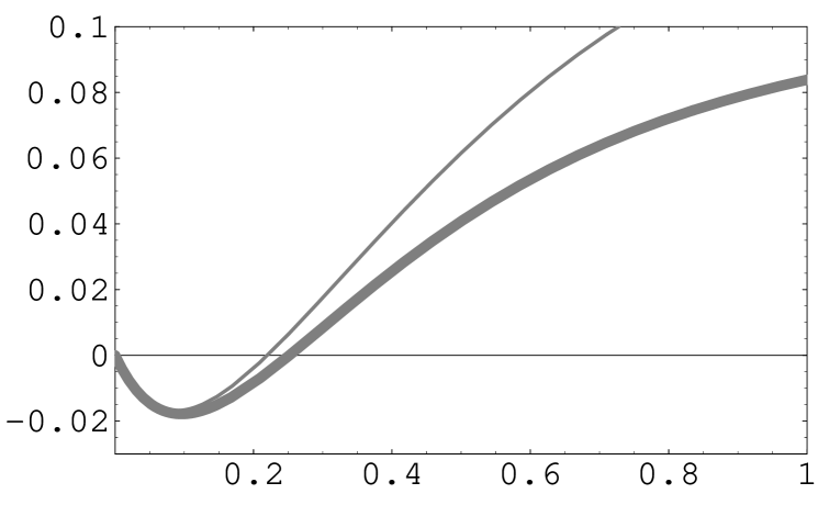
Figure 1: Our description of $\Gamma^{p}_{1}(Q^{2})$ versus $Q^{2}$. The thick line is the new analysis to be compared with the thin line, which represents our previous approach without corrections.

Here we took the asymptotic value for $\Gamma_{1}^{p}=0.147$ providing the good description of $\Gamma_{1}^{p}(Q^{2})$ for $Q^{2}$ of the order of several $GeV^{2}$, when the 3-loops radiative correction is included. This procedure may be considered as a sort of preliminary estimate, since the full 3-loops analysis is not available.

To generalize our approach to the neutron case, we use the difference between proton and neutron instead of the neutron itself. Although it is possible, in principle, to construct a smooth interpolation for the functions $g_{1}$ themselves [17], it does not fit the suggested general argument on the linearity in $\mu_{A}$, since $I^{p-n}_{1}(0)$ is proportional to $\mu_{A,n}^{2}-\mu_{A,p}^{2}$, which is quadratic and, moreover, has an additional suppression due to the smallness of isoscalar anomalous magnetic moment. So we suggest the following parametrization for the isovector contribution of $I_{T}(Q^{2})$, namely $I^{p-n}_{T}(Q^{2})$, above the matching point, where again only the 1-loop term is presented explicitly

$$I^{p-n}_{T,pert}(Q^{2})=\theta(Q^{2}-Q^{2}_{1}){2M^{2}\over{Q^{2}}}[\Gamma^{p-n}_{1}(1-\frac{\alpha_{s}(Q^{2})}{2\pi})$$

$$-c_{p}\frac{<<O_{p}>>}{Q^{2}}+c_{n}\frac{<<O_{n}>>}{Q^{2}}-I^{p}_{2}(Q^{2})+I_{2}^{n}(Q^{2})].$$ (18)

Here the transition value $Q_{1}^{2}$ may be determined by the continuity conditions in a similar way. We get the value $Q_{1}^{2}\sim 1.04\mbox{GeV}^{2}$, which is not too far from that of the proton case. Concerning $I_{2}^{n}(Q^{2})$, which is given by Eq. (8), we have not neglected $G_{E}^{n}(Q^{2})$ and we have used its very recent determination [19]. The result of this calculation is very slightly modified compared to the case where one assumes $G_{E}^{n}(Q^{2})=0$ and all the subsequent results involving the neutron were obtained with a non-zero $G_{E}^{n}(Q^{2})$. The asymptotic value of $\Gamma_{1}^{p-n}=0.21$ is dictated by the Bjorken sum rule. We also took the same value $<<O_{n}>>=0.11\mbox{GeV}^{2}$ as in the proton case. The plot representing $\Gamma^{p-n}_{1}(Q^{2})$ is displayed on Fig. 2 and agrees well with the very recent experimental data [20].

This may be considered as an argument in favour of the general picture of power corrections obtained in QCD sum rules calculations [14], where the neutron correction is small. However the quantitative comparison with the calculations in the framework of the chiral soliton model [18] would require a more detailed analysis.

Now we have all the ingredients to turn to the behavior of neutron integral, which is simply obtained from the difference $\Gamma_{1}^{p}(Q^{2})-\Gamma_{1}^{p-n}(Q^{2})$. It is shown on Fig. 3 and we notice that the strong oscillation around $Q^{2}=1\mbox{GeV}^{2}$, we had in the previous analysis, is no longer there.

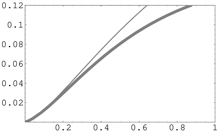
Figure 2: Our prediction for $\Gamma_{1}^{p-n}(Q^{2})$ versus $Q^{2}$. The thick line is the new analysis to be compared with the thin line, which represents our previous approach without corrections.

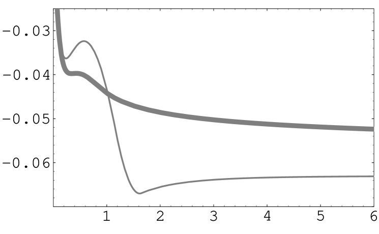
Figure 3: Our prediction for $\Gamma_{1}^{n}(Q^{2})$ versus $Q^{2}$. The thick line is the new analysis to be compared with the thin line, which represents our previous approach without corrections.

We now have all the ingredients to investigate the deuteron integral. Note that in this case the generalization of the GDH sum rule may be naturally decomposed into two distinct regions.

The first one is the region of large $Q^{2}$, where nuclear binding effects can be disregard, so that the deuteron structure function is the simple additive sum of the proton and neutron ones. As a result, the $Q^{2}\to 0$ limit of this intermediate asymptotics is defined by the sum of the squares of proton and neutron anomalous magnetic momenta.

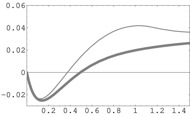
Figure 4: Our prediction for $\Gamma_{1}^{d}(Q^{2})$ versus $Q^{2}$. The thick line is the new analysis to be compared with the thin line, which represents our previous approach without corrections.

When nuclear binding effects are taken into account one should get instead the square of the sum of these anomalous magnetic moments. As they are known to be rather close in magnitude and of different sign, the result should be therefore very small.

The difference between these two regimes should be attributed [21] to the deuteron photodesintegration channel, which is supported by existing explicit calculations [22] in the case of real photons. For virtual photons, this allows to estimate the $Q^{2}$ value, where binding effects start to play a role, to be of the order of $m_{\pi}^{2}$. The simplest way to implement this reasoning [21] is to use the following expression:

$$I^{d}_{1}(Q^{2})=\frac{1}{2}[\theta(Q_{d0}^{2}-Q^{2})\frac{2Q^{2}}{Q_{d0}^{2}+Q^{2}}+\theta(Q^{2}-Q_{d0}^{2})](I^{p}_{1}(Q^{2})+I^{n}_{1}(Q^{2})$$ (19)

Here we introduced the nuclear scale $Q_{d0}\sim m_{\pi}$ and neglected the square of the deuteron anomalous magnetic moment. The prediction is shown in Fig. 4 and seems to be in good agreement with the preliminary JLAB data [23].

Let us finally discuss the role of the elastic contribution. It must be definitely included [24] if one uses the operator product expansion (OPE),  which is the essential tool in determining the power corrections. However, we use the OPE only above matching point, where the elastic contribution is small. At the same time, below the matching point the object those $Q^{2}$ behaviour is studied may be considered as a sort of fracture function, where only a partial summation over final states, excluding the elastic one, is implied. It is this function which may reach the GDH value at $Q^{2}=0$.

Acknowledgments

We are indebted to Vladimir Braun, Volker Burkert, Claude Bourrely, Gail Dodge, Sebastian Kühn and Zein-Eddine Meziani for discussions and correspondence. O.T. is indebted to CPT for warm hospitality and financial support. He was also partly supported by RFBR (Grant 03-02-16816) and by INTAS (International Association for the Promotion of Cooperation with Scientists from the Independent States of the Former Soviet Union) under Contract 00-00587.

References

- [1] S. B. Gerasimov, Yad. Fiz. 2, 598 (1965) [Sov. J. Nucl Phys. 2, 430(1966)].
- [2] S. D. Drell and A. C. Hearn, Phys. Rev. Lett. 16, 908 (1966).
- [3] E143 Collaboration, K. Abe et al., Phys. Rev. Lett. 78, 815 (1997).
- [4] E94010 Collaboration, M. Amarian et al., Phys. Rev. Lett. 89, 242301 (2002).
- [5] HERMES Collaboration, A. Airapetian et al., Phys. Lett. B494, 1 (2000); Eur. Phys. J. C26, 527 (2003).
- [6] CLAS Collaboration, J. Yun et al., Phys. Rev. C67, 055204 (2003) and R. Fatemi et al., Phys. Rev. Lett. 91, 222002 (2003).
- [7] J. Soffer and O. Teryaev, Phys. Rev. Lett. 70, 3373 (1993).
- [8] J. Soffer and O. Teryaev, Phys. Rev. D51, 25 (1995).
- [9] A. L. Kataev, G. Parente and A. V. Sidorov, Nucl. Phys. B573, 405 (2000).
- [10] H. Burkhardt and W. N. Cottingham, Ann. Phys. (N.Y.) 16, 543 (1970).
- [11] J. Schwinger, Proc. Nat. Acad. Sci. U.S.A. 72, 1559 (1975).
- [12] J. Soffer and O. Teryaev, Phys. Lett. B545, 323 (2002).
- [13] V. D. Burkert and B. L. Ioffe, Phys. Lett. B296, 223 (1992) and J. Exp. Theor. Phys. 78, 619 (1994) [Zh. Eksp. Teor. Fiz. 105, 1153 (1994)]; V.D. Burkert and Z. Li Phys. Rev. D47, 46 (1993). V. D. Burkert, AIP Conf. Proc. 603, 3 (2001) and Nucl. Phys. A699, 261 (2002).
- [14] V. M. Braun and A. V. Kolesnichenko, Nucl. Phys. B283, 723 (1987).
- [15] S. Simula, M. Osipenko, G. Ricco and M. Taiuti, Phys. Rev. D65, 034017 (2002)
- [16] S. A. Larin, F. V. Tkachov and J. A. Vermaseren, Phys. Rev. Lett. 66, 862 (1991); S. A. Larin and J. A. Vermaseren, Phys. Lett. B259, 345 (1991).
- [17] B. L. Ioffe, V. A. Khoze and L. N. Lipatov, Hard Processes, (North-Holland, Amsterdam, 1984). Nucl. Phys. B283, 723 (1987).
- [18] N. Y. Lee, K. Goeke and C. Weiss, Phys. Rev. D65, 054008 (2002).
- [19] R. Madey et al., Phys. Rev. Lett. 91, 122002 (2003).
- [20] A. Deur et al., arXiv:hep-ex/0407007.
- [21] O. V. Teryaev, arXiv:hep-ph/0303003.
- [22] H. Arenhövel, arXiv:nucl-th/0006083.
- [23] G. Dodge, talk at GDH2004, June 2-5 2004, Old Dominion University.
- [24] X. D. Ji and W. Melnitchouk, Phys. Rev. D56, 1 (1997).